Faculty of Electrical Engineering,
Mathematics & Computer Science
Designing a small and low-energy
wild life tag for parakeets within
an urban environment
capable of tracking and
online activity recognition
R.T. van den Berg M.Sc. Thesis
August 2019
This project has been an interesting learning experience for me and has taught me many things. I have learned a great deal about planning a large project, and I have learned a lot about analyzing and gathering data. Especially keeping up with reports is something to take into account.
I want to offer my thanks to dr. Nirvana Meratnia for supervising me throughout this master thesis. She gave me great advice and offered new insights into my research.
Next, I would like to thank prof. dr. ir. Paul Havinga for offering this opportunity and setting the basis for this research.
I want to thank dr. Bert Toxopeus for arranging the parakeet for our measure-ments.
For the hardware aspects of this project, I want to thank dr. ir. Wouter van Kleunen for providing the tags and helping me develop a better understanding of practical embedded systems.
I also genuinely want to thank ir. Jacob Kamminga for his always helpful ad-vice and being there to answer every random question. This helped me to keep motivated, and we always had great discussions.
I want to thank dr. ir. Kyle Zhang for his last minute help in the design of the tag. Next, I want to thank my late grandfathers Mathieu Schlangen and Arend van den Berg for their continuous interest in my technical studies.
Finally, I would like to thank my family, friends, and girlfriend for their continued support throughout this thesis. When motivation got low, they helped me get it back.
This work is concerned with designing and building an online activity classifier and tracking device on an embedded system to monitor parakeets. This involves the de-sign choices in localization, feature selection, classifying algorithm and optimization of required features and algorithm parameters. In order to reduce the number of in-puts to a machine learning algorithm, Forward Selection was applied, which reduced the number of features from 20 to 7. The resulting feature sets were then applied to six learning algorithms; k-Nearest Neighbours, Naive Bayes, Neural Network, Linear Discriminant Analysis, Decision Tree, and Support Vector Machine. In order to eval-uate the machine learning algorithm, data from a parakeet was used for training and testing using a 70% to 30% ratio, creating a generic classifier which could accurately recognise the activity of a parakeet. The models were evaluated and compared ac-cording to three main metrics, namely performance, battery usage, and ease of implementation, as well as other metrics such as variance in performance, usability and training effort.
It was found that the combination of the decision tree classifier with seven time-domain features from the accelerometer’s 3D vector magnitude comprised the best compromise between the evaluated metrics. The decision tree parameters were tuned such that its performance could be maintained while minimizing the tree size. A window size of two seconds and a 50% window overlap was used to yield an ex-cellent compromise between computation and performance. The accuracy of clas-sification varied between 87 and 90%.
Next, satellite-, ground-based- and radar tracking methods were compared in terms of energy consumption and accuracy. A localization system has been pro-posed based on the received signal strength of Bluetooth Low Energy beacons. These beacons were detectable from a 40-meter distance.
Finally, this tracking device and online activity classifier have been implemented on the AKMW-iB001M beacon, and the performance will be tested in the future on wild parakeets in M´alaga, Spain.
Acknowledgements iii
Abstract v
List of acronyms ix
1 Introduction 1
1.1 Target animals . . . 3
1.2 Research question . . . 4
1.3 Report organization . . . 4
2 State Of The Art 5 2.1 Techniques . . . 5
2.1.1 Location Tracking . . . 5
2.1.2 Data preprocessing . . . 9
2.1.3 Classification Algorithms . . . 11
3 Hardware selection 13 3.1 Requirements . . . 13
3.2 Transmission . . . 14
3.3 Power supply . . . 14
3.4 Placement . . . 15
3.5 Hardware versus weight . . . 16
3.6 Hardware selection . . . 17
3.7 Location Tracking . . . 18
4 Methods 21 4.1 Data Collection . . . 21
4.1.1 Owl . . . 21
4.1.2 Falcon . . . 22
4.1.3 Parakeet . . . 22
4.2 Data Labelling . . . 23
4.3 Data Processing & Feature Selection . . . 26 4.4 Algorithm Training . . . 28 4.5 Tracking . . . 29
5 Results 33
5.1 Behaviour Classification . . . 33 5.2 Tracking . . . 34 5.3 Implementation . . . 34
6 Conclusions and discussion 41
6.1 Conclusions . . . 41 6.2 Discussion . . . 42
References 45
Appendices
A Appendix 53
AAR Animal Activity Recognition
AoA Angle of Arrival
BLE Bluetooth Low Energy
CPU Central Processing Unit
DSC Doppler Shift Calculations
DT Decision Tree
FN False Negative
FP False Positive
GPS Global Positioning System
GSM Global System for Mobile Communications
ISS International Space Station
k-NN k-Nearest Neighbours
LDA Linear Discriminant Analysis
LZO Lempel-Ziv-Oberhumer
LZW Lempel-Ziv-Welch
NB Naive Bayes
NN Neural Network
RAM Random Access Memory
RSS Received Signal Strength
SVM Support Vector Machine
TDoA Time Difference of Arrival
ToF Time of Flight
UHF Ultra High Frequency
Introduction
Animal behaviours and activities are essential to better understand the species and their environment [1], [2]. For example, social scientists are turning to animal be-haviour as a framework in which to interpret human society and its problems [3]. Many problems in human society are often related to the interaction of environment and behaviour or genetics and behaviour. Another example is that of Sir Charles Sherrington [4]. He developed a model for the structure and function of the nervous system based on close behavioural observation of animals. Other research showed that animal behaviour could tell about the animals’ health [5] and their social in-teractions [1]. Activity recognition might also be implemented to protect animals from poachers [6]. Finally, the behaviour and activities of animals often provide early warning signs of environmental degradation. Changes in sexual and other be-haviour occur much sooner at lower levels of environmental disruption than changes in reproductive outcomes and population size [7].
Therefore, many scientists collect data on these behaviours and activities on ways varying from making notes with pen and paper to using collars with sensors. One of the oldest techniques is to observe the animal by human observers over a long time [8]–[11]. An issue with this technique is the human-dependency, which re-quires an observer to be present at all times to monitor the animals’ activity. Human observation is not only tricky but also impractical, especially when such an animal moves to locations restricted to humans or travels with high speed. Another issue is that the animal might behave differently in the presence of a human (which pri-marily is the case for wild animals). Another observation technique is to observe via cameras. This eliminates the problem of a human observer needing to be present at all times and causes no influence on the behaviour and activity of the animal. The animal can be filmed, and later its behaviour and activities can be classified. However, with cameras, one is bounded to a fixed area and can therefore only be used on animals in captivity or restricted to a space. Finally, collars can be used to collect information on the behaviours and activities of animals. With this, a small
device is secured onto the animal with various sensors attached to it. These sen-sors gather various kind of data (e.g. movement, location, temperature) about the animal. The animal always carries the collar along, providing more information than human observations and cameras.
Sensors in the collar gather a large amount of data. To interpret this sensor data into animal behaviours and activities, one uses machine learning. Machine learning looks for patterns in the data symbolizing certain activities (e.g. walking, standing,
flying, swimming). This classification is often performed offline, after retrieval of
the sensor data. Retrieval of the data is done either via removing the sensor or transmitting the raw data wireless for offline analysis. Wireless transmission is costly in terms of energy. Therefore, processing sensor data on an embedded system can be cheaper in terms of energy demand instead of sending the raw data over a radio. Many applications would benefit from live updates regarding an animals activity, for instance, to notice environmental disasters, such as forest fires.
Animal Activity Recognition (AAR) is achieved by processing sensor data on a device on the animal. Subsequently, the activities periodically transmit the animals’ behaviours and activities. Therefore, the embedded device needs to compute and classify the gathered data continuously. These devices are limited in terms of stor-age, power and computational resources. This poses the challenge to design a sophisticated learning algorithm on a non-intrusive and low-energy system.
Another way to get insight into the behaviour of animals is location tracking. Lo-cation tracking supports tackling the many environmental challenges we currently face, including problems posed by invasive species [12], [13], the spread of zoonotic diseases [14] and declines in wildlife populations due to anthropogenic climate and land-use changes [15].
1.1 Target animals
Worldwide, there are about 350 species of parrots and parakeets (order: Psittaci-formes). In total, 54 of these species have been introduced to areas outside their native ranges, and 38 species have become established in the non-native range [16]. Humans exhibit ambivalent feelings toward parrots and parakeets. Many of these birds are strikingly beautiful and highly prized as companion animals, while others are banned because of potential agricultural damage or competition with na-tive species. Many parrot species are afforded special protection because they are endangered in their native habitats. Often these species are considered crop pests and persecuted by farmers [17].
The monk parakeet (Myiopsitta monachus) and rose-ringed parakeet (Psittacula krameri) are undoubtedly the worlds most successfully introduced parrot species. Each species now enjoys a broad non-native range where conflicts with human activity include crop damage [18], competition with native species [12], [13], and property damage [19]. Each species exemplifies invasiveness through its capacity to adapt to new conditions and to exploit opportunities created by human activity. Biologists and resource managers are challenged to develop and implement effec-tive strategies that not only protect resources from these invasive species but also account for public opinions, which often favour the charismatic avian invaders.
Eliminating small populations of these birds is the primary strategy to deal with their immense growing population. The main problem with dealing with these para-keets is the lack of information on the birds. While there have been previous studies into the monk parakeet and rose-ringed parakeet, they are either outdated [20]–[22], or only look at global patterns [12], [23] or are observatory studies [8]–[11] leaving space for human error.
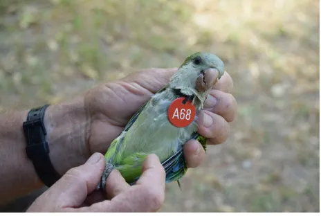
Currently, the University of M´alaga is trapping monk parakeets and tying neck-collars around the birds (see Figure 1.1). By marking these birds, they get certain primitive information. However, observatory studies do not supply enough informa-tion. To get a better understanding of the monk parakeets’ location, behaviour and activities need to be analysed.
Figure 1.1:A parakeet with a neck-collar
The main body of this thesis deals with the different design aspects of such an AAR system. This includes the choice of hardware, infrastructure and the activity recognition. Finally, a prototype of the system is built and evaluated.
1.2 Research question
Within this study, we answer the following research question:
What level of online activity recognition performance can be achieved for birds while tracking locations in urban environments?
Sub questions include:
• How can a bird activity recognition system be implemented on a small,
light-weight and low-power embedded device?
• What are the trade-offs between accuracy and functionality against weight and
energy?
• How to minimize the required localization infrastructure?
1.3 Report organization
State Of The Art
This chapter discusses the state-of-the-art of data loggers and the used techniques of those loggers. We divide the state-of-the-art section in location tracking, data preprocessing and behaviour classification.
2.1 Techniques
2.1.1 Location Tracking
Within this part, we classify tracking systems (see figure 2.1) in the way they derive location data: 1) satellite tracking, 2) local tracking, 3) radar tracking. All techniques and specifications are further elaborated by Bridge et al. [24].
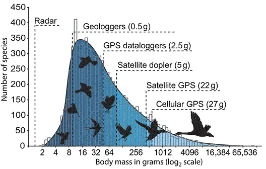
First, we look at satellite tracking, which is suitable for real-time tracking, but very costly in terms of power and money. One can do animal tracking through the Global Positioning System (GPS) [25]–[27] or through the Doppler Shift Calculations (DSC) [28], [29]. While GPS is very accurate (accuracy at 5m vs 100m-50km compared to DSC), it also uses much power and therefore needs a bigger battery. The smallest GPS tags at present are in the 20 to 150-gram range, which limits their application to larger animals (> 200g). Another difference when comparing GPS to DSC is
the number of fixes per day. DSC is only able to do this once a day, while GPS can get multiple fixes throughout the day. Therefore, DSC is unfit for tracking small movement but great for migratory movement.
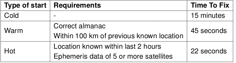
When choosing for GPS, there is a difference among a cold start, warm start and a hot start [30]. At a cold start, the GPS does not know where on earth it is located and has no clear idea where the satellites are. Therefore, the GPS locates a satellite to connect to so it can get a general impression of its location. When connected to a satellite, it will request the almanac, which contains the approximate information on all the other satellites locations. In total, the time to get a fix from the start-up is about 15 minutes. Next, we have a warm start; with this, the GPS already has the correct
Type of start Requirements Time To Fix
Cold - 15 minutes
Warm Correct almanac
Within 100 km of previous known location 45 seconds
Hot Location known within last 2 hours
[image:16.595.64.463.86.194.2]Ephemeris data of 5 or more satellites 22 seconds
Table 2.1: Different types of GPS start-ups
almanac data and a previous location within 100 km of the current location. Then it asks the ephemeris data from the satellite which contains that satellite’s detailed orbital information. The time to get the first fix with a warm start is only 45 seconds. Finally, there is a hot start. With this, a position was determined within the previous 2 hours, and the GPS has the ephemeris data of at least five satellites. Now time to a first fix takes about 22 seconds. Table 2.1 gives an overview of these three types. Using local tracking gives some options which require less power than GPS. Here we can use tower identification, Bluetooth and Wi-Fi identification, radio teleme-try, acoustic telemeteleme-try, magneto-inductive tracking, dead-reckoning and solar ge-olocating. Tower identification (or radio-tracking) [31] is the most straightforward tracking system since one only needs to identify with which tower the tag is con-nected. However, this is not always doable due to coverage issues and support of mobile companies. Detailed movement can not be tracked this way since these towers cover a large area. On the other hand, it works well in urban areas, which are always covered. Another option is the use of Bluetooth [32], [33] or Wi-Fi [34]. By measuring the received signal strength of different beacons, one can determine where a device is located. Bluetooth is a better option for bird tracking since it re-quires less power than Wi-Fi. How detailed a location can be tracked depends on the amount of Bluetooth tags spread out through the area. Therefore, the main issue is that it can only be used in a predetermined area. However, the technique excels in individual movement tracking.
is that it is very susceptible to multipath fading. Also, the tag needs to send out a signal and then download each position circle, making it power expensive. A simi-lar technique called Time Difference of Arrival (TDoA) [35] is mainly used in GPS. The tag measures the difference in time of arrival between two or more signals. By using this data, the tag can calculate its position relative to the signal sources. The location of the signal sources needs to be known in order for this to work. One of the major disadvantages in this technique is jitter, a small variation in the frequency of the output signal. While the tag does not need to send out any signal, these com-putations itself can be power expensive. Another technique is to use the Received Signal Strength (RSS)/fingerprinting [36]. This technique knows each RSS on any location. By comparing the RSS to the known ’map’, one can determine its location. This technique is mainly used indoors since each location needs to be measured be-forehand. It is also possible without such a ’map’ by computing the distance through the RSS and loss. Like ToF, this makes it susceptible to multi-path fading and adds extra computations. Finally, Angle of Arrival (AoA) [35] can be used to calculate the angle of incidence of an incoming signal with respect to a reference. This method is mainly used in DSC. It calculates position in one of two ways. In the first method, the AoA and ToF information is combined, resulting in the position of the tag in polar coordinates. The main advantage is that only one node is necessary to determine the location, but has the same disadvantages as ToF. The other way two or more AoA stations are set up at known distances from each other, the AoA of an incoming signal is calculated at each station, and the position of the tag is calculated through triangulation. The advantage here is the lack of time components, using angles only leaving space for jitter and a-synchronization. The disadvantage is that the AoA stations must have a fixed reference for the calculated angles to have any meaning, limiting the measurable area.
Figure 2.1: Tracking system classification
systems, there is only one active tracking system, called magneto-inductive tracking [41]. Localization of mobile devices underground is exceptionally challenging, with radio propagation severely attenuated by soil and moisture. Therefore, magnetic fields are placed above grounds which penetrate the ground, and these strengths are recorded and sent when the animal is above ground. A more passive tracking option is dead-reckoning [42]. Dead-reckoning uses a known start position and de-rives the new positions through the use of the animals’ speed, heading and change in height with respect to the previous positions. This system does not require a lot of battery power and can, therefore, work over a long time. Due to a variable (wind) speed or drift the errors in position are very high [43]. A solution for this could be to make an independent fix through GPS at regular intervals. However, this would bring back the weight problem. Finally, we have a solar geolocator [44], which tracks its latitude through the length of the day and longitude through the time of solar noon. This is again a cheap and small system, which does not require a lot of bat-tery power. However, the accuracy can range from 50km to 200km, and it can only locate a bird once per day, making it inadequate for tracking local movement.
animals like insects. Finally, no additional tags need to be present on the animal itself. However, radar tracking also has its limitations. They are more suited to track masses than individuals, and the radar is bound to a particular area. Also, no other information can be derived than an animals location. Furthermore, the current in-frastructure is mainly focussed on aerial species, while there are certainly options for maritime species.
2.1.2 Data preprocessing
Current sensing technology has enabled to monitor animal behaviour and activities with the help of accelerometers [25], [26], [38], [46]–[49], cameras [38], [50], mi-crophones [38]–[40], thermal sensors [48], barometers [51] and EEGs [46] among others.
With all this sensor information, one can identify different behaviours. This identi-fication is accomplished by manually comparing their behaviour with the data, which is feasible for a limited dataset and behaviours; as done by Bouten et al. [25] and Sheppard et al. [49]. However, with large sets of data, it is easier to do this through machine learning. We will elaborate on this in the next section.
When tracking an animals location and behaviour, much data is generated. To deal with this, either a large memory is needed, some data processing needs to be applied, or frequent transmissions need to take place. A good option would be to include a large memory if no form of transmission is used, making the total tag power efficient. However, if no recapturing of the animal for data recollection is necessary, forms of data processing or data compression need to be used.
The simplest data processing technique is to take the mean of values over a pe-riod (windowing) and not send all raw values. A much-used technique is to calculate the 3D-vector and its features over a small time window (1-2 seconds). These time and frequency-domain features are typically used in activity recognition [24], [25], [41], [48], [49], [52]. Another idea is to cut down on the sampling frequency. For in-stance, Nathan et al. [53] sample their accelerometers for durations of 16.2 seconds at 10-minute intervals. This sampling technique gives a grainy resolution, but a high resolution is not always necessary. Finally, one can already compute the necessary data for the research locally. Again Nathan et al. calculate ’roost arrival time’, ’daily travelled distance’, ’maximal displacement’ and ’flight straightness’ locally and only stores and transmits these values.
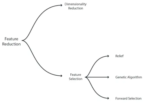
princi-Figure 2.2: Overview of feature reduction techniques
pal components, which are sets of linearly uncorrelated values with a covariance of 0. Then these components are ranked by their variance. Dimensionality reduc-tion can be useful when working with many features from the same domain to filter out duplicate features. Feature selection can be done through relief [55], genetic algorithms [56] or forward selection [57], all different methods which choose fea-tures which contribute the most towards classification accuracy. Relief estimates the quality and relevance of features by their ability to classify and discriminate be-tween similar classes. Relief is excellent to predetermine the used features. Next, genetic algorithms choose a random amount of features and see which features score the highest in terms of classification performance. The higher features are retained for the next generation until an optimum is found. The main problem might be that one can reach a local optimum. Finally, forward selection selects features one by one and evaluates their performance according to a classifier. Again the highest performing features are added to the selection. However, here the problem might be that discarded features cannot be re-selected, thus again only reaching a local optimum. Bisby [58] compares these techniques on accuracy and execution time. She shows that forward selection results in the lowest execution time while still retaining accurate accuracy.
[image:20.595.161.409.105.284.2]algorithms, we will not further investigate those.
2.1.3 Classification Algorithms
In section 2.1.2, we looked at different sensors, feature selection and data compres-sion. The next step is to classify the animals’ activity through a machine learning algorithm. First, we will discuss all relevant algorithms, including the AAR that use these algorithms. Then we show relevant research comparing or evaluating these al-gorithms. The most used algorithms are k-Nearest Neighbours (k-NN), Naive Bayes (NB), Decision Tree (DT), Neural Network (NN), Support Vector Machine (SVM) and Linear Discriminant Analysis (LDA).
k-NN searches the training data points to find k data points closest to an incoming data point in order to predict it. These k training examples are called the k ”nearest neighbours” of the incoming data point. k-NN is easy to implement for multi-class problems, requires no training step and uses instance-based learning. The con-straints of the algorithm are that it is a slow algorithm (especially as datasets grow), does not perform well on imbalanced data and is very sensitive to outliers. Bidder et al. [60] tests k-NN in AAR for badgers, camels, cormorants, dingos, kangaroos, wombats and humans. While they reach high accuracy for kangaroos and humans (91% and 95% respectively), the average accuracy lays at 78%. The two aerial species, cormorant and wombat, reach an accuracy of 77% and 76% respectively, showing worse results than the average performance.
NB builds a simplistic probability model which assumes that features are inde-pendent and evaluates them indeinde-pendently. It also works well in multi-class prob-lems; it is easy to understand and can work on any size dataset. The cons are the assumption of independence class features (which is never the case in real life), and the algorithm suffers fromZero Frequency [61]. Browning et al. [62] use NB to
determine whether the location of diving behaviour can be predicted from GPS data across three seabird species. NB predicted only non-dives well (85-95% accuracy), but did poorly on predicting dives with only 40% accuracy. The author claims this due to the unbalanced data set.
NN replicates a network containing layers, in which several nodes are connected with each neuron on the preceding and succeeding layer. Each connection has a defined weight on which the feature is multiplied with, leading to a final classification result. The algorithm outperforms almost every other machine learning algorithm and is widely used in the offline machine learning. However, NN requires more training data than other machine learning algorithms, acts as a black box and is computationally expensive. While we can find many types of research comparing NN to other algorithms [53], [68], [69], no implemented versions are presented up to now.
SVM aims to maximise the margin between training patterns and the decision boundary and drawing hyperplanes between classes. SVM focusses on data points which are from different classes but are close together, in comparison to other algo-rithms which focus on all data points. The algorithm is useful in the higher dimen-sion, when classes are separable and when the number of features is higher than the training examples. However, it is difficult to find the appropriate hyperparameters and kernel function and does not perform well in case of overlapped classes. Goa et al. [70] build a web-based tagging and AAR system. They train an SVM through data from humans, dogs and badgers all with an accuracy of over 90%. Lee et al. [71] show an implemented version of an SVM to measure aggression of pigs, with an accuracy of 95,2%.
LDA expresses one dependent feature as a linear combination of other indepen-dent features, forming a set of continuous indepenindepen-dent features which define class labels, aiming to distinguish between independent and dependent features. The al-gorithm works well if the class conditional densities of clusters are approximately normal, also when there are more features than training examples. LDA fails to find the lower-dimensional space if the dimensions are much higher than the number of samples in the data matrix. Next, it also suffers from to discriminate between non-linearly separable classes. Also, Viazzi et al. look into pig aggression, classi-fying with an LDA with 89% accuracy. This version is no implemented version as presented by Lee et al..
Kamminga et al. [69] compare seven different machine learning algorithms for their behaviour classification. They look at memory usage, Central Processing Unit (CPU) execution time, accuracy and F-scores. It shows that the NB algorithm is the cheapest to use in terms of resource usage, closely followed by DT, NN and Deep Neural Networks. Bisby [58] shows the same results but also includes an implemented version of the DT algorithm.
Hardware selection
Within this chapter, we will sketch the requirements for a wildlife tag and explain what hardware fulfils these requirements.
3.1 Requirements
When measuring on animals, ethical rules apply to protect the animal. The foremost rule is the maximum weight that may be added to the animal. For birds, this is 5% of the total weight. Since parakeets weigh around 150 gram, our tag can weigh 7,5 gram at maximum.
To get an overview of the daily activities of the parakeet, we want to log its lo-cation and real-time classify its activities. The importance of these parameters are explained in chapter 1. Next, to get a better overview of these activities, we want to see if specific patterns emerge. With a month worth of data, we believe to have enough data to get a better insight into the behaviour of the parakeet.
Finally, the parakeet is returning to its nest each night, but to capture them is quite tricky. To decrease the chance of data loss, we want to download the data from a distance, instead of trying to recapture the bird for tag retrieval.
For the tag to be used on rose-ringed and monk parakeets the following require-ments apply:
• The tag must weigh 7,5g at maximum.
• The tag should operate for at least one month.
• Data should be downloadable from a distance (no tag retrieval).
• The tag should be able to log its location.
• The tag should be able to real-time classify the activity from the animal.
3.2 Transmission
The gathered raw accelerometer data needs to be recovered from the device. There are two main options with each having its implementations again. The options are satellite systems and ground-based receivers.
The first option is the use of satellite systems. These systems can update real-time and send their data over a satellite link. This option gives an up-to-date overview of each tracked individual. However, as can be imagined, these systems have high costs and power requirements. An existing application which uses a satel-lite system is the ICARUS initiative [72]. The ICARUS initiative is a tag connected to a module on the International Space Station (ISS), mainly focussed on bio-logging. The main difference between conventional satellite systems is that the ISS is closer to the earth and thus needs less power to communicate.
The other option is the use of ground-based receivers. These are less power expensive than satellite systems but do allow downloading the data real-time. The only issue might be coverage since not all networks are available at every place, especially in maritime areas. The most common transmitter is the Global System for Mobile Communications (GSM) transmitter since the GSM network is available worldwide. Next, we have radio telemetry as described in section 2.1.1. Radio telemetry can only be used when the transmitter is in the neighbourhood and can not handle a large number of data transmissions. Finally, there are other long-range transmission protocols like Amber Wireless, Ingenu, LoRa, NWave, Platanus and Sigfox as described by Baharudin and Yan [73]. These ground-based receivers fit well into our wanted application since they are power efficient and do not require tag retrieval.
To circumvent transmission altogether, one can also do tag retrieval. With this technique, tags only store the gathered information. After some time the animal must be recaptured so the tag can be recovered and data can be downloaded. Overall this is an alternative method for wireless monitoring. This technique is suited for homebound animals or when using a recovery beacon. This is not very well suited for parakeets since it is hard to catch them.
3.3 Power supply
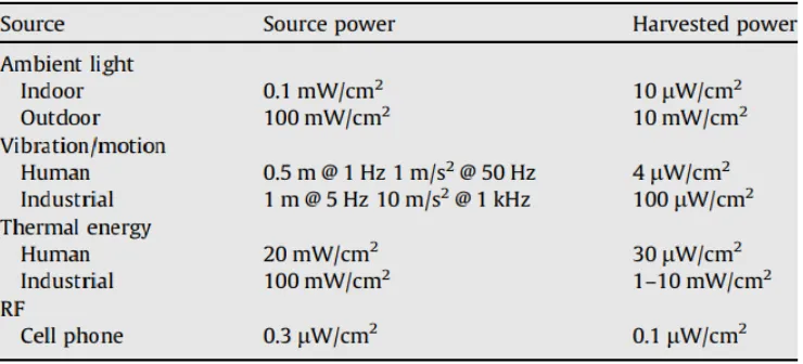
Figure 3.1: Characteristics of various energy sources available in the ambient and harvested power. [75, Table 2]
or shorten the time when measuring or use power-efficient algorithms. Next, Mitche-son et al. [74] classify charging methods into electromagnetic radiation (RF), thermal gradients, light and motion. All techniques can be found in Figure 3.1.
Ambient RF is the most underdeveloped technique and still struggles with de-livering significant power levels. Thermoelectric generation works well but is much dependent on the direct change in temperature. Solar power has the highest power levels and is mainly used in bio-logging [25], [72], [76]. The two constraints for solar power are light availability, especially for animals living in darker parts of the world, and the price of solar cells. Finally, there is motion-based energy harvesting, which is less efficient than solar energy harvesting but is less dependent on external fac-tors. All these techniques increase the lifetime of the tag, but also the complexity.
Two techniques are generally used for power, one being solar power and the other only using a battery. Other techniques can also be used depending on the bird. For instance, RF can be placed underneath the nest if one is tracking a homebound bird (such as the parakeet). Thermoelectric generation can be used by placing one element on the bird and the other element exposed to the wind/environment. How-ever these last two techniques have problems delivering significant power levels.
3.4 Placement
With all hardware in place, the next question will be to look at the placement and attachment of the device. Different attachment methods used in bio-logging are:
• Harness
• Epoxy glue
• Glue
• Suction cup
• Dorsal fin clamp
• Rubber cement
• Attached to antlers
Not every one of these methods is suited for every species in bio-logging.
Some attachment methods are meant to release within a specific time, while others need to stay in place until they can be retrieved. Concerning the first method, it is also essential that the device is biodegradable or has a beacon so it can be retrieved.
Placement is also crucial in influencing the behaviour of an animal. Such a tag is extra weight for an animal making it less aerodynamic and having a higher energy expenditure. Next, some places are not fit for a tag due to characteristic behaviour of a species, like diving or digging.
Placement is a significant issue with birds since it can influence its behaviour and foraging. Vandenabeele et al. [77] claim that for plunge-diving birds, the tag can be best placed on the lower back while for strictly flying birds, the middle back is the right spot. Other places like the head, tail or belly give too much drag or do not stay put when diving. What is not taken into account is the effect on the measurements when placing these devices. For instance, Rattenborg et al. [46] use electroencephalography (EEG), which can be best placed on the head of a bird. Also, an accelerometer records more detailed movement when placed closer to the head than the lower back, making it possible to identify different kinds of behaviour precisely.
3.5 Hardware versus weight
Figure 3.2: The frequency distribution of bird body masses (in grams) in relation to possible tracking technologies. Minimum bird sizes for each technology are represented according to the 5%-body-weight rule. [24, Figure 1]
3.6 Hardware selection
We used the AKMW-iB001M beacon from AnkhMaway (see Figure 3.3) since it ful-filled all requirements. The tag weighs 6g, falling in the 0-7,5g range. Through the 3-axis accelerometer, we can measure the displacement of the bird and use it to classify behaviour. The working time of the tag is 4.63 months based on a broad-casting rate of one second. Since we broadcast less but have more substantial computations, we suspect this will suffice for at least one month. Finally, it broad-casts with Bluetooth Low Energy (BLE) 4.0, which can be used to track location (as described in Section 2.1.1) and transmits its gathered data (as described in Section 3.2) from a distance. Moreover, the tracking will be discussed in Section 3.7. The full specifications of the tag can be found in Appendix A.1. No comparison was made with other tags.
The tag works well. It has a Bluetooth range of 50m, and the energy consumption of the accelerometer is very sparse. While it is difficult to use for attachment, it is light-weight. Finally, the tag is not perfect for development since no schematics are available.
suf-Figure 3.3: The AKMW-iB001M beacon open and closed respectively.
fice all requirements. For both tags, no schematics are available since both were commercially bought.
The Axy-Trek sensor was a perfect tag to do quick measurements. It had an easy to handle user interface and did not have any problematic initialization parts. Also, settings could be changed through the user interface, and rings were available for attachment. However, as stated before the battery life was poor (5-6 hours) and data could only be downloaded from the tag after capturing the bird, making it unsuited for wild parakeets.
For location tracking, we use standard MiniBeacons. It runs on two AA batteries and is easy to replace. Moreover, the precise working of location tracking can be found in the next section.
3.7 Location Tracking
We track location via Bluetooth identification (again, as described in Section 2.1.1). Bluetooth beacons (as described in Section 3.6) send out an advertisement signal. This signal broadcasts that they are there. The tag will pick up this signal and add it to its log. Since the tag only needs to listen and does not need to broadcast, the operation is power-efficient. The Minibeacons have a theoretical range of maximum 70 m. Often, this range is smaller due to natural obstacles and reflection. Therefore, the practical range is about 50m, covering about one hectare of land. The idea is to put up a grid of beacons with 100 m in between each beacon. An overview of such a grid is visible in Figure 3.4, for 24 hectares of land.
[image:28.595.115.457.87.224.2]Methods
The state-of-the-art in section 2 gives a clear overview of all available techniques. Next, we look at which of these are suitable for parakeet activity recognition and describe our used methods. We start with how we obtained the training data, next selected the features and show the developed algorithm. Finally, we show our how we tested our tracking part.
4.1 Data Collection
In total, we did three measurements on three different bird species. We tested on an owl, a falcon and a parakeet. During each measurement, data collection was done with the Axy-Trek logger, as explained in section 3.6. For our measurements, only the accelerometer was activated since the other sensors were not available on the development tag, the AKMW-iB001M. The accelerometer was sampled at 100 Hz, with a G fullscale of 8g and an 8-bit resolution, resulting in a timestamp and accelerometer values for the x-,y- and z-axis.
4.1.1 Owl
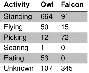
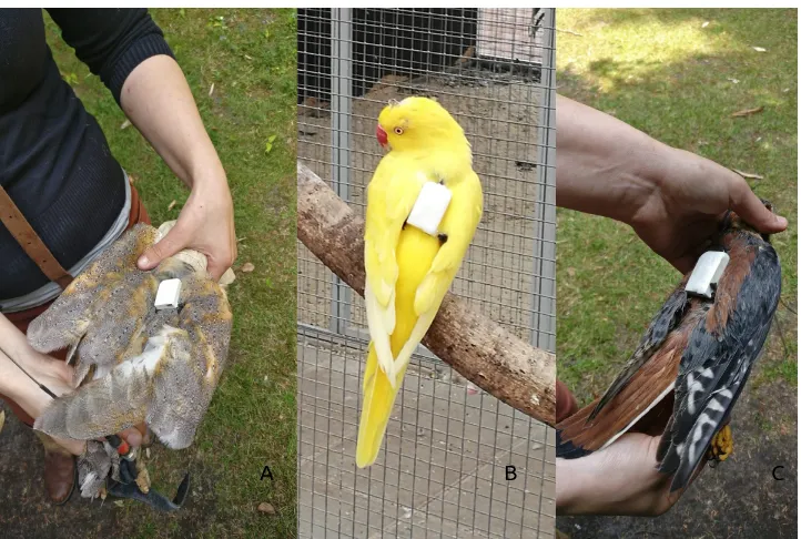
The first measurement took place in ”Wonderwereld”, a small zoo in Ter Apel (Nether-lands), with the permission from the park’s owner. The logger was placed on the back of the owl (see Figure 4.1A). One manually controlled camera was used to fol-low the bird. The measurement with the owl was done in the open air, with the help of one of the zookeepers. In this way, the owl would perform actions on command, resulting in an equal distribution of activities. Measurements were done for 30 min-utes after which the owl refused to follow commands. Therefore, the experiment was seized. Within this time, no sufficient data to train a machine-learning algorithm was gathered. We will give a small overview of the measured activities in Table 4.1.
Activity Owl Falcon Standing 664 91 Flying 50 15 Picking 12 72 Soaring 1 0 Eating 53 0 Unknown 107 345
Table 4.1: Data entries per activity of the owl and falcon
4.1.2 Falcon
Since our target animal was not available in this first measurement, we also mea-sured on a falcon. ”Falcons have a similar wing frequency as parakeets”, according to the bird expert B. Toxopeus. Therefore, we expect that the activities of a falcon produce the same data as those of a parakeet. Also, we used the data from the falcon to compare it to the owl so that we could use the data gathered from the owl within our algorithm training.
This measurement also took place in ”Wonderwereld”, directly after the mea-surement with the owl. The logger was placed on the back of the falcon (see figure 4.1C). Also, one manually controlled camera was used to follow the falcon around. A dead-spot was present in the corner above the camera. The falcon was placed in a small cage of ∼ 20m2, with a height of 3m, limiting the time of flights. Only
10 minutes of data were gathered since the available zookeeper had to go, and no experiments were allowed without their supervision. The gathered data is in Table 4.1.
4.1.3 Parakeet
The owl data and the falcon data were nothing alike, and thus, both datasets were excluded in the research. Therefore, a third measurement needed to take place. This time a rose-ringed parakeet was available (see figure 4.1B). The measure-ments took place at the ”World of Birds foundation”, a bird welfare foundation in Erica (Netherlands), with permission from the foundation’s owner. The bird was able to move around freely within a cage of∼70m2, with a height of3m. Within the cage,
Figure 4.1: F.l.t.r. The tagged owl, the tagged parakeet, the tagged falcon
In total, around 941500 raw data points were collected. Statistics on these data entries can be found in figure 4.2. This shows all gathered activities in a 3D-scatter graph. Clear distinctions between standing, flying and shaking are visible, while the rest of the activities are tightly grouped. A logarithmic scale was used to show this grouping better. The activities that were observed during the day are listed in Table 4.2. These are labelled activities, which took place over 2 second windows.
4.2 Data Labelling
In order to use supervised learning methods, each data point must contain an ad-ditional label field indicating the class to which it belongs according to the ground-truth. Therefore, the ground-truth is deduced by video footage of the parakeet, which is synchronised with the sensor data. The labelling of the data was done through a Matlab GUI developed by Jacob Kamminga, allowing the annotation of the data according to video footage [52]. This labelling was done manually, and an example of the GUI can be seen in figure 4.3. While this GUI was initially used for labelling data sets of goats [69], it worked well for labelling bird activities with minimum mod-ifications to the code.
Activity Description
Standing The animal is standing still, occasionally adapting its posture. Flying The animal is flying and is not in contact with the ground.
Picking The animal picks with its beck. This is done either to see if it can remove the tag or to put its feathers straight.
Shaking The animal is shaking its entire body in a very rapid motion. Jumping The animal jumps up or down from one place to another. Climbing The animal moves across or up/down a branch or fence.
Walking The animal walks across the ground without using its wings. The pace is almost always the same.
Scratching The animal scratches its head/body with its claw. Eating The animal eats some seads.
[image:36.595.64.535.95.335.2]Unknown Any other activity which could not be placed properly underneath the mentioned activities above.
Table 4.2: Observed activities during the day
tion was unclear, it would be labelledunknown.
4.3 Data Processing & Feature Selection
[image:36.595.64.534.99.334.2]The dataset of the parakeet was segmented according to the labelling file. The segments were split into 70% training data and 30% test data. Data were segmented with a two-second window size and a 100 Hz sample rate. We overlap consecutive windows to alleviate the effects of edge conditions, which occur when windows are segmented sequentially. Therefore, segments are generated with an overlap size of 50%.
Table 4.3 shows the number of data points for each class for both the training and testing data. Noticeable is the lack of entries for jumping, shaking, scratching and eating. These four activities did not take place for longer than 2 seconds or did not occur so often. Therefore, we will reduce the classification activities to six classes;
standing,flying, picking, climbing,walking andother (which includejumping,
shak-ing,scratching,eatingandunknown).
Activity Training set Testing set
Standing 4256 1767
Flying 96 50
Picking 760 325
Shaking 4 1
Jumping 0 0
Climbing 354 181
Walking 111 32
Scratching 9 1
Eating 28 2
[image:37.595.201.425.86.279.2]Unknown 177 123
Table 4.3: Data entries per activity of the parakeet
slightly balanced.
Balance = H logk =
−Pk i=1
Ci
n log Ci
n
logk (4.1)
Finally, we calculate the time domain and frequency domain features for each window. Table 4.4 gives an overview of which features are calculated and adds a small description per feature. These features are used to train our algorithms. However, since we do not want to use all features on our embedded platform due to energy constraints, we do three tests. The first test includes all features, the second only frequency-domain features and the final test only time-domain features. We test this for NN, DT and SVM since they are the three most commonly used algorithms. Finally, we compare F1-scores and accuracy versus the required power.
We also apply forward selection (as described in section 2.1.2) to see if we can reduce our feature set. Forward selection selects the following features:
• Mean
• Standard Deviation
• 25 percentile
• Skewness
• Principal frequency
• Frequency Entropy
Feature Description
Maximum Maximum value
Minimum Minimum value
Mean Average value
Standard deviation Amount of variation
Median Middle value
25 percentile Value below which 25% of the observations are found 75 percentile Value below which 75% of the observations are found Mean low pass filtered signal Mean value of DC components
Mean rectified high pass filtered signal Mean value of rectified AC components
[image:38.595.69.501.84.319.2]Skewness of the signal The degree of asymmetry of the signal distribution Kurtosis The degree of ’tailedness’ of the signal distribution Principal frequency Frequency component with the greatest magnitude Spectral energy The sum of squared discrete FFT component magnitudes Frequency entropy Measure of the distribution of frequency components Frequency magnitudes Magnitude of the first six components of FFT analysis
Table 4.4: All calculated features for each window
These might be the best features, but still, a combination of time-domain and frequency-domain features are used. Therefore, we repeat the same process only with time-domain features (which are also less battery expensive operations). This time the following features are selected:
• Minimum
• Standard Deviation
• Median
• 25 Percentile
• 75 Percentile
• Skewness
• Kurtosis
4.4 Algorithm Training
Figure 4.4: Example of a process in Rapidminer
We compare the algorithms mentioned in Section 2.1.3. The basic parameters are used in Rapidminer, and each algorithm uses the same features as explained in Section 4.3. Therefore, results will not be optimal for each algorithm. The six algorithms will be tested on the same data set of the parakeet. The best performing one will be optimized and then implemented on the wildlife tag.
4.5 Tracking
To determine the range of the Minibeacons, we put three Minibeacons in an open square and measured the RSS. The measurements were done on the O& O-square on the University of Twente (see Figure 4.5). This is a square where many people and thus signals pass-by, simulating an urban environment. Three Minibeacons were placed at one end of the square and measurements were done at 1, 11, 21, 31, 41 and 51 m distance. Each measurement was done twice, resulting in six measurements per position.
Results
Within this section, we show the performance of the behaviour classification and our final implementation.
5.1 Behaviour Classification
We compare the use of different features sets as described in Section 4.3, all with the parakeet dataset. The results are visible in Figure 5.1. As accuracy only gives a prediction on the correctly predicted observations, we also want to include our False Positive (FP) and False Negative (FN). Therefore, we include an average F1-score. Equation 5.1 is used to calculate the F1-score.
P recision= T P
T P +F P Recall = T P
T P +F N F1 = (P recision
−1+Recall−1
2 )
−1
(5.1)
We see a clear difference in the F1 scores when only time-domain features are used; however, the accuracy stays around the same. Another thing to note is that the NN performs better overall except when the time-domain features are used. While it is clear that the best performance is given by using all the features, we choose to use only time-domain features since they are computationally inexpensive. In the following experiments, we use the forward selection feature set described in Section 4.3.
Figure 5.2 shows the average accuracy and F1-score of our trained algorithms. We notice for other activities almost no correct predictions are made in this class.
This has multiple reasons. First of all, not much data is available for this class (see table 4.3). Next, all data points are spread out and thus non-consistent when training the algorithm. Finally, many of theseother activities resemble one of the other five
Figure 5.1:Performance of DT, NN and SVM with different feature sets
activities. For instance, the activity shaking looks like flying and eating like picking. Therefore, we also included the F1-score without the other activities. For further
graphs, all F1-scores are calculated without theother category.
The top three performers are NB, NN and DT. k-NN, LDA and SVM had difficul-ties in distinguishing walking from picking and climbing.
5.2 Tracking
As described in Section 4.5, we measure the RSS to determine the range of the MiniBeacons. Figure 5.3 shows the results of this experiment. During the experi-ments it was sunny and about We did not receive any beacon at the 51-meter dis-tance; therefore, it is not included in the graph. On 41 meter, we received only one beacon. The RSS of the other two beacons has been set to -110 dB to better depict the situation.
The range, therefore, is a maximum of 40 meters.
5.3 Implementation
Figure 5.2: The performance of the different machine learning algorithms
[image:45.595.134.493.471.694.2]Parameter Description Value Splitting criterion The criterion which decides which attributes will be selected for splitting. Information gain
Maximal depth The depth of a tree varies depending upon the size and characteristics of the ExampleSet.This parameter is used to restrict the depth of the decision tree. 9
Apply pruning Branches are replaced by leaves according to the confidence parameter after generation of the model. True
Confidence This parameter specifies the confidence level used for the pessimistic error calculation of pruning. 0.4
Apply prepruning
This parameter specifies if more stopping criteria than the maximal depth should be used during generation of the decision tree model.
If true, the parameters minimal gain, minimal leaf size, minimal size for split and number of prepruning alternatives are used as stopping criteria.
True
Minimal gain
The gain of a node is calculated before splitting it. The node is split if its gain is greater than the minimal gain.
A higher value of minimal gain results in fewer splits and thus a smaller tree.
0.1
Minimal leaf size
The size of a leaf is the number of Examples in its subset.
The tree is generated in such a way that every leaf has at least the minimal leaf size number of Examples.
2
Minimal size for split The size of a node is the number of Examples in its subset.Only those nodes are split whose size is greater than or equal to the minimal size for split parameter. 4
[image:46.595.67.508.83.270.2]Number of prepruning alternatives When split is prevented by prepruning at a certain node this parameter will adjustthe number of alternative nodes tested for splitting. 10
Table 5.1: Decision Tree parameters
However, the DT was implemented via nested conditional statements for decisions. Again 2 second windows were used since historically this proved most effective. No other values were tested. A visual implementation of the DT can be found in Ap-pendix A.2. We tuned the parameters for the best settings with a grid search [80]. We used the accuracy of the algorithm versus tree size as our performance metric when tuning the parameters. A short description of each parameter and the final value can be found in Table 5.1.
As mentioned in Section 4.1, we also recorded data from a falcon and an owl. We added this to the training data to see if our results increased. The result can be found in figure 5.4.
Noticeable is the drop in precision and recall when the owl data is included. The falcon data increases our performance slightly and can be beneficial for our algorithm. However, all results with falcon data are within the error margin and thus not significant. We also look at similar activities and how well our classifier could recognize the activities. For the activities of the owl, we could predict the activities ’flying’ and ’standing’ with an average precision and recall of 97% and an overall accuracy of 80%. Other activities from the owl, like ’soaring’ and ’eating’, were only predicted with an average precision and recall of 4%. These activities are performed differently by owl and parakeet; therefore, the low precision and recall make sense. Activities of the falcon had a high precision from 98%. However, recall dropped to 75% and only a total accuracy of 60% was reached. We suspect this low accuracy comes from the use of a small data set.
This algorithm is implemented on the AKMW-iB001M beacon. Every 5 seconds, we classify two seconds of data. The classification is stored together with a se-quence number.
Figure 5.4: Performance of the decision tree with data from other birds included
Figure 5.5: The 26 bytes which are stored
quick to implement and does not have complex computations. Every 5 seconds a scan is done for all different BLE devices in the neighbourhood. If the name of the tag starts with ’Minibeacon’, the RSS value, the last byte of the address and a sequence number are stored. By linking the sequence numbers from the DT classifier and the tracker, we can determine where each activity took place. An example of a stored operation can be seen in Figure 5.5.
A high-level overview of the code can be found in Figure 5.6.
The current code takes up 90 kB flash memory and 14 kB Random Access Memory (RAM). Leaving 160 kB flash memory open for storage. Around 6000 store operations can be done before the memory is full. If every 5 seconds a scan is done, about 8 hours of measurements can be done before the memory is full. We expect this is enough to measure the daily activities of a bird. At the end of the day, the data will be offloaded, and the memory is cleared.
[image:47.595.96.576.369.458.2]Conclusions and discussion
This chapter consists of conclusions about the results presented in Chapter 5 and gives some recommendations for future research.
6.1 Conclusions
Within this thesis, we showed the development of an AAR system for parakeets including location tracking. We implemented an AAR system for parakeets on an embedded device with a decision tree classifier. We have shown that with simple statistical time-domain features, it can compete with more sophisticated algorithms such as NN and SVM in terms of performance. While frequency-domain features performed better on F1-scores, each algorithm showed no significant differences in accuracy. To answer our main research question”How can a bird activity recognition
system be implemented on a small, light-weight and low-power embedded device?”,
we first answer each subquestion.
What are the trade-offs between accuracy and functionality against weight and
energy? Sophisticated localisation techniques deliver better results but do require
too much energy to be applicable. We used a low energy Bluetooth protocol to de-termine the location on a smaller scale. This protocol was well suited for parakeets since they are non-migratory birds. Again, this works less than solutions with GSM, but the energy constraint weighs more substantial than the accuracy. Another exam-ple of the energy constraints is that of the activity classifier. NN reached the highest accuracy but was not implemented since DT is more energy-efficient than NN. The main reason to design the tag power-efficient is the limiting hardware possibilities. As discussed before, the weight restriction resulted in a tag without a large battery. To let the tag operate at least one month, every operation needed to be low-power. Also, not much memory could be included, again limiting the tag. We minimized the loss in accuracy, but we can conclude that the weight and energy, weigh more
substantial on the design of the tag than the accuracy and functionality.
When looking at the necessary localization infrastructure, again the trade-off be-tween energy and functionality comes up. We chose to include more localization points to decrease the needed energy. The beacons only had a reach of 40 me-ter, which is significantly smaller than the theoretical 70 meters. The schematic that has been introduced (see figure 3.4) works well for small areas and minimizes the needed infrastructure. If one needs to measure on a broader scale, we suggest leav-ing more space in between the beacons. This gives a grainy resolution but keeps the same amount of required infrastructure. Another option is to put the beacons on locations which are known to be visited by the birds.
Looking at online activity recognition, we get a high accuracy for our decision tree. We reach an average accuracy of 87,35% for our parakeet dataset. An F1-score of 54,9 is obtained, which can be increased by filtering out other activities.
Online activity recognition is possible for birds, but there are a lot of similar activities (except for flying and standing). These activities sometimes overlap (e.g. climbing and picking) and are hard to distinguish. Similar behaviour of the algorithm can also be seen when testing on the owl and falcon dataset. Flying and standing are distinct activities, while the other activities often overlap (see Figure 4.2). Overall we can accurately determine which activity is performed, but there is room for improvement for the other activities.
In the end, we can conclude that a bird activity recognition system can be imple-mented on a small, light-weight and low-power embedded device. The main issue with this implementation is the weight restriction of 5%, limiting the tracking and clas-sifying techniques. However, with the use of low-power methods like BLE and DT, no massive battery is needed, while maintaining excellent performance.
6.2 Discussion
First of all, no final tests have been performed on birds with the designed tag. While it has the same algorithm running as the previous, we can not be sure the performance will match this tag. The designed tag will be tested and evaluated in the future on wild parakeets in M´alaga, Spain. We look forward to seeing the results.
are now hard to classify due to the low number of samples and are merged into
other activities.
Next, the mentioned localization techniques like AoA and TDoA increase the accuracy of tracking. In our proposed system the RSS is stored, indicating the distance to the beacon. However, with AoA, the angle can be determined and give a precise location of the tag.
Finally, the ICARUS project (as mentioned in Chapter 2 is a promising project to use GPS while remaining energy efficient. Unfortunately, our tag was not suited for this project. We highly recommend seeing if a tag can be designed in combination with this project.
[1] J. Alcock and D. R. Rubenstein,Animal behavior. Sinauer Associates
Sunder-land, MA, USA, 2019.
[2] Y. Sahin, “Animals as mobile biological sensors for forest fire detection,” Sen-sors, vol. 7, no. 12, pp. 3084–3099, 2007.
[3] T. Wey, D. T. Blumstein, W. Shen, and F. Jordan, “Social network analysis of animal behaviour: a promising tool for the study of sociality,” Animal behaviour,
vol. 75, no. 2, pp. 333–344, 2008.
[4] R. E. Burke, “Sir charles sherrington’s the integrative action of the nervous system: a centenary appreciation,”Brain, vol. 130, no. 4, pp. 887–894, 2007.
[5] B. L. Hart, “Biological basis of the behavior of sick animals,” Neuroscience &
Biobehavioral Reviews, vol. 12, no. 2, pp. 123–137, 1988.
[6] J. Kamminga, E. Ayele, N. Meratnia, and P. Havinga, “Poaching detection tech-nologies - a survey,”Sensors (Switserland), vol. 18, 5 2018.
[7] D. J. Rapport, H. A. Regier, and T. Hutchinson, “Ecosystem behavior under stress,”The American Naturalist, vol. 125, no. 5, pp. 617–640, 1985.
[8] J. M. South and S. Pruett-Jones, “Patterns of flock size, diet, and vigilance of naturalized monk parakeets in hyde park, chicago,”The Condor, vol. 102, no. 4,
pp. 848–854, 2000.
[9] J. L. Navarro, M. B. Martella, and E. H. Bucher, “Breeding season and produc-tivity of monk parakeets in cordoba, argentina,” The Wilson Bulletin, pp. 413–
424, 1992.
[10] L. F. Mart´ın and E. H. Bucher, “Natal dispersal and first breeding age in monk parakeets,”The Auk, pp. 930–933, 1993.
[11] J. Postigo, A. Shwartz, D. Strubbe, and A.-R. Mu˜noz, “Unrelenting spread of the alien monk parakeet myiopsitta monachus in israel. is it time to sound the alarm?,” Pest management science, vol. 73, pp. 349–353, 02 2017.
[12] D. Strubbe and E. Matthysen, “Invasive ring-necked parakeets psittacula krameri in belgium: habitat selection and impact on native birds,” Ecography,
vol. 30, pp. 578 – 588, 08 2007.
[13] K. Freriks, “Is de overlast van halsbandparkieten echt zo erg?,”NRC, Jan 2019.
[14] H. Kruse, A.-M. Kirkemo, and K. Handeland, “Wildlife as source of zoonotic infections,”Emerging infectious diseases, vol. 10, no. 12, p. 2067, 2004.
[15] T. L. Benning, D. LaPointe, C. T. Atkinson, and P. M. Vitousek, “Interactions of climate change with biological invasions and land use in the hawaiian islands: modeling the fate of endemic birds using a geographic information system,”
Proceedings of the National Academy of Sciences, vol. 99, no. 22, pp. 14246–
14249, 2002.
[16] P. Cassey, T. M. Blackburn, D. Sol, R. P. Duncan, and J. L. Lockwood, “Global patterns of introduction effort and establishment succes in birds.,” vol. 271, 2004.
[17] J. Tella, A. Rojas, M. Carrete, and F. Hiraldo, “Simple assessments of age and spatial population structure can aid conservation of poorly known species,”
Bi-ological Conservation, vol. 167, pp. 425 – 434, 2013.
[18] M. Conroy and J. C. Senar, “Integration of demographic analyses and decision modeling in support of management of invasive monk parakeets, an urban and agricultural pest,”Environmental and Ecological Statistics, vol. 3, pp. 491–510,
12 2009.
[19] M. Avery, J. Lindsay, J. Newman, S. Pruett-Jones, and E. Tillman, “Reducing monk parakeet impacts to electric utility facilities in south florida,”Advances in
Vertebrate Pest Management, vol. 4, pp. 125–136, 01 2006.
[20] C. Leveret al.,Naturalized animals of the British Isles. Hutchinson, 1977.
[21] C. Lever, “Ring-necked parakeet (psittacula krameri). naturalized birds of the world,” 1987.
[22] J. L. Long, “Introduced birds of the world: The worlwide history, distribution and influence of birds introduced to new environments.,” 1981.
[23] D. Strubbe and E. Matthysen, “Establishment success of invasive ring-necked and monk parakeets in europe,” Journal of Biogeography, vol. 36, no. 12,
[24] E. S. Bridge, K. Thorup, M. S. Bowlin, P. B. Chilson, R. H. Diehl, R. W. Fl”´e”ron, P. Hartl, R. Kays, J. F. Kelly, W. D. Robinson, et al., “Technology on the move:
recent and forthcoming innovations for tracking migratory birds,” Bioscience,
vol. 61, no. 9, pp. 689–698, 2011.
[25] W. Bouten, E. W. Baaij, J. Shamoun-Baranes, and K. C. J. Camphuysen, “A flexible gps tracking system for studying bird behaviour at multiple scales,”
Jour-nal of Ornithology, vol. 154, pp. 571–580, Apr 2013.
[26] R. Kays, P. A. Jansen, E. M. Knecht, R. Vohwinkel, and M. Wikelski, “The effect of feeding time on dispersal of virola seeds by toucans determined from gps tracking and accelerometers,” Acta Oecologica, vol. 37, no. 6, pp. 625–631,
2011.
[27] P. E. Clark, D. E. Johnson, M. A. Kniep, P. Jermann, B. Huttash, A. Wood, M. Johnson, C. McGillivan, and K. Titus, “An advanced, low-cost, gps-based animal tracking system,” Rangeland Ecology & Management, vol. 59, no. 3,
pp. 334–340, 2006.
[28] C. Vincent, B. J. Mcconnell, V. Ridoux, and M. A. Fedak, “Assessment of argos location accuracy from satellite tags deployed on captive gray seals,” Marine
Mammal Science, vol. 18, no. 1, pp. 156–166, 2002.
[29] A. S. Fischbach, S. C. Amstrup, and D. C. Douglas, “Landward and eastward shift of alaskan polar bear denning associated with recent sea ice changes,”
Polar Biology, vol. 30, no. 11, pp. 1395–1405, 2007.
[30] Surveylab, “Gps ttff and startup modes.” https://www.measurementsystems. co.uk/docs/TTFFstartup.pdf. Accesed: 2018-10-15.
[31] G. C. White and R. A. Garrott,Analysis of wildlife radio-tracking data. Elsevier,
2012.
[32] A. Huhtala, K. Suhonen, P. M¨akel¨a, M. Hakoj¨arvi, and J. Ahokas, “Evaluation of instrumentation for cow positioning and tracking indoors,” Biosystems
Engi-neering, vol. 96, no. 3, pp. 399–405, 2007.
[33] B. Thorstensen, T. Syversen, B. Evjemo, O. Johnsen, T. G. Solvoll, S. Akselsen, A. Munch-Ellingsen, and H. Karlsen Jr, “System and method for tracking indi-viduals,” Oct. 17 2006. US Patent 7,123,153.
[34] M. Mustafa, I. Hansen, and S. Eilertsen, “Animal sensor networks: Animal wel-fare under arctic conditions,”,” in SENSORCOMM 2013: The Seventh
[35] T. T. Brooks, H. H. Bakker, K. Mercer, and W. Page, “A review of position track-ing methods,” in1st International conference on sensing technology, pp. 54–59,
2005.
[36] I. Alyafawi, “Towards self-learning radio-based localization systems,” pp. 556– 557, 03 2012.
[37] R. Kays, S. Tilak, M. Crofoot, T. Fountain, D. Obando, A. Ortega, F. Kuem-meth, J. Mandel, G. Swenson, T. Lambert,et al., “Tracking animal location and
activity with an automated radio telemetry system in a tropical rainforest,”The
Computer Journal, vol. 54, no. 12, pp. 1931–1948, 2011.
[38] J. Krause, S. Krause, R. Arlinghaus, I. Psorakis, S. Roberts, and C. Rutz, “Re-ality mining of animal social systems,” Trends in ecology & evolution, vol. 28,
no. 9, pp. 541–551, 2013.
[39] M. Campbell and C. M. Francis, “Using microphone arrays to examine effects of observers on birds during point count surveys,”Journal of Field Ornithology,
vol. 83, no. 4, pp. 391–402, 2012.
[40] D. J. Mennill and S. L. Vehrencamp, “Context-dependent functions of avian duets revealed by microphone-array recordings and multispeaker playback,”
Current Biology, vol. 18, no. 17, pp. 1314–1319, 2008.
[41] A. Markham, N. Trigoni, D. W. Macdonald, and S. A. Ellwood, “Underground localization in 3-d using magneto-inductive tracking,” IEEE Sensors Journal,
vol. 12, no. 6, pp. 1809–1816, 2012.
[42] O. Bidder, J. Walker, M. Jones, M. Holton, P. Urge, D. Scantlebury, N. Marks, E. Magowan, I. Maguire, and R. Wilson, “Step by step: reconstruction of ter-restrial animal movement paths by dead-reckoning,”Movement ecology, vol. 3,
no. 1, p. 23, 2015.
[43] R. P. Wilson, E. Shepard, and N. Liebsch, “Prying into the intimate details of animal lives: use of a daily diary on animals,” Endangered Species Research,
vol. 4, no. 1-2, pp. 123–137, 2008.
[44] E. Rakhimberdiev, N. Senner, M. A. Verhoeven, D. Winkler, W. Bouten, and T. Piersma, “Comparing inferences of solar geolocation data against high-precision gps data: Annual movements of a double-tagged black-tailed godwit,”