Original citation:
Malkhozov, Aytek, Mueller, Philippe, Vedolin, Andrea and Venter, Gyuri. (2016) Mortgage risk and the yield curve. Review of Financial Studies, 29 (5). pp. 1220-1253.
Permanent WRAP URL:
http://wrap.warwick.ac.uk/94011
Copyright and reuse:
The Warwick Research Archive Portal (WRAP) makes this work by researchers of the University of Warwick available open access under the following conditions. Copyright © and all moral rights to the version of the paper presented here belong to the individual author(s) and/or other copyright owners. To the extent reasonable and practicable the material made available in WRAP has been checked for eligibility before being made available.
Copies of full items can be used for personal research or study, educational, or not-for profit purposes without prior permission or charge. Provided that the authors, title and full bibliographic details are credited, a hyperlink and/or URL is given for the original metadata page and the content is not changed in any way.
Publisher’s statement:
This is a pre-copyedited, author-produced version of an article accepted for publication in Review of Finance following peer review. The version of record Aytek Malkhozov, Philippe Mueller, Andrea Vedolin, Gyuri Venter; Mortgage Risk and the Yield Curve, The Review of Financial Studies, Volume 29, Issue 5, 1 May 2016, Pages 1220–1253,
https://doi.org/10.1093/rfs/hhw003 is available online at: http://dx.doi.org/10.1093/rfs/hhw003
A note on versions:
The version presented here may differ from the published version or, version of record, if you wish to cite this item you are advised to consult the publisher’s version. Please see the ‘permanent WRAP url’ above for details on accessing the published version and note that access may require a subscription.
Mortgage Risk and the Yield Curve
∗
Aytek Malkhozov
†Philippe Mueller
‡Andrea Vedolin
§Gyuri Venter
¶Abstract
We study the feedback from the risk of outstanding mortgage-backed secu-rities (MBS) on the level and volatility of interest rates. We incorporate the supply shocks resulting from changes in MBS duration into a parsimonious equilibrium dynamic term structure model and derive three predictions that are strongly supported in the data: (i) MBS duration positively predicts nominal and real excess bond returns, especially for longer maturities; (ii) the predictive power of MBS duration is transitory in nature; and (iii) MBS convexity increases interest rate volatility, and this effect has a hump-shaped term structure.
∗We would like to thank Tobias Adrian, Caio Almeida, Michael Bauer, Ruslan Bikbov, Mike
Cher-nov, John Cochrane, Pierre Collin-Dufresne, Jefferson Duarte, Greg Duffee, Mathieu Fournier, Andr´as F¨ul¨op, Robin Greenwood, Sam Hanson, Christian Julliard, Anh Le, Neil Pearson, Douglas McManus, Marcel Rindisbacher, Richard Stanton, Dimitri Vayanos, Nancy Wallace, Paul Whelan, two anonymous referees, and seminar and conference participants at the Bank of England, Banque de France, CBS, Deutsche Bank, Duke University, Erasmus University, Exeter University, Imperial Business School, LSE, Manchester Business School, the Oxford-MAN Institute, Toulouse School of Economics, Luxembourg School of Finance, University of Nottingham, SAC Capital Advisors, University of Bern, University of Bonn, 2012 Arne Ryde Workshop, 2012 IFSID Conference on Structured Products and Derivatives, 2012 Young Scholars Nordic Finance Workshop, 2012 Junior Faculty Research Roundtable at UNC, 2012 Conference on Advances in the Analysis of Hedge Fund Strategies, 2013 Mathematical Finance Days, 2013 Bank of Canada Fixed Income conference, 2013 Financial Econometrics conference in Toulouse, 2013 SFS Cavalcade, 2013 WFA meetings, 2013 UNC/Atlanta Fed Conference on Housing, 2014 NBER SI AP, and 2015 AFA Meetings for thoughtful comments. Malkhozov gratefully acknowledges finan-cial support from the Institut de Finance Math´ematique de Montr´eal. Mueller and Vedolin gratefully acknowledge financial support from the LSE Research Committee Seed Fund. Venter gratefully ac-knowledges financial support from the Center for Financial Frictions (FRIC), grant no. DNRF102. All authors thank the Paul Woolley Centre at the LSE and the Dauphine-Amundi Chair in Asset Man-agement for financial support. The views expressed in this paper are those of the authors and do not necessarily reflect those of the Bank for International Settlements.
†Bank for International Settlements, Centralbahnplatz 2, 4002 Basel, Switzerland, Phone: +41 61
280 864, Email: aytek.malkhozov@bis.org
‡London School of Economics, Department of Finance, Houghton Street, WC2A 2AE London, UK,
Phone: +44 20 7955 7012, Email: p.mueller@lse.ac.uk
§London School of Economics, Department of Finance, Houghton Street, WC2A 2AE London, UK,
Phone: +44 20 7955 5017, Email: a.vedolin@lse.ac.uk
¶Copenhagen Business School, Department of Finance, Solbjerg Plads 3, 2000 Frederiksberg,
Mortgage-backed securities (MBS) and, more generally, mortgage loans constitute a
major segment of US fixed income markets, comparable in size to that of Treasuries. As
such, they account for a considerable share of financial intermediaries’ and institutional
investors’ exposure to interest rate risk.1 The contribution of MBS to the fluctuations in
the aggregate risk of fixed income portfolios over short to medium horizons is even more
important. Indeed, because most fixed-rate mortgages can be prepaid and refinanced as
interest rates move, the variation of MBS duration can be very large, even over short
periods of time.2
In this paper we study the feedback from fluctuations in the aggregate risk of MBS
onto the yield curve. To this end, we build a parsimonious dynamic equilibrium term
structure model in which bond risk premia result from the interaction of the bond
supply driven by mortgage debt and the risk-bearing capacity of specialized fixed income
investors.
The equilibrium takes the form of a standard Vasicek (1977) short rate model
aug-mented by an affine factor, aggregate MBS dollar duration, which captures the additional
interest rate risk that investors have to absorb. Intuitively, a fall in mortgage duration
is similar to a negative shock to the supply of long-term bonds that has an effect on
their prices. In addition to duration itself, its sensitivity to changes in interest rates,
measured by aggregate MBS dollar convexity, also plays a role. Because MBS duration
falls when interest rates drop, mortgage investors who aim to keep the duration of their
portfolios constant for hedging or portfolio rebalancing reasons will induce additional
buying pressure on Treasuries and thereby amplify the effect of an interest rate shock.
As a result, the MBS channel can simultaneously affect bond prices and yield volatility.
1
Between 1990 and 2014 the average value of outstanding mortgage-related and Treasury debt was USD 5tr each. Financial intermediaries and institutional investors hold approximately 25% of the total amount outstanding in Treasuries, and approximately 30% of the total amount outstanding in MBS. Government-sponsored enterprises (GSEs) hold on average around 13% of all outstanding MBS (see Securities Industry and Financial Markets Association (2013) and the Flow of Funds Tables of the Federal Reserve).
2
Our model makes a range of predictions for which we find strong empirical evidence.
First, MBS duration predicts both nominal and real bond excess returns. This effect
is stronger for longer maturity bonds that are more exposed to interest rate risk. At
the same time, the effect is weaker for real bonds if real rates are imperfectly correlated
with nominal rates and are less volatile. Accordingly, we find an economically significant
relationship between duration and bond risk premia, in particular at longer maturities:
A one standard deviation change in MBS duration implies a 381 basis point change in
the expected one-year excess return on a 10-year nominal bond and a 199 basis point
change in the expected one-year excess return on a 10-year real bond. These effects
imply an approximately 38≈381/10 (20) basis point increase in nominal (real) 10-year
yields, assuming that most of the effect on returns happens within a year.
Second, while large in size, shocks to MBS duration and their effect on bond excess
returns are transient. Our model captures the fast mean-reversion in aggregate MBS
duration by linking it to both interest rate mean-reversion and the renewal of the
mort-gage pool through refinancing. For example, running predictive regressions for different
return horizons, we find little additional effect of MBS duration on bond excess returns
beyond one year.
Finally, in our model the feedback between changes in long-term yields and MBS
duration translates into higher yield volatility: Lower interest rates decrease duration,
which in turn decreases the term premium and further lowers long-term rates. Different
from noncallable bonds, callable bonds such as MBS typically feature a concave
relation-ship between prices and yields, the so-called negative convexity. More negative convexity
implies that the duration and, therefore, the market price of risk are more sensitive to
changes in interest rates. Empirically, we find that the effect is hump-shaped and most
pronounced for maturities between two and three years. In terms of magnitude, any one
standard deviation change in MBS dollar convexity changes 2-year bond yield volatility
by approximately 37 basis points. A calibrated version of our model reproduces the
above predictions with similar economic magnitudes.
The statistical significance and the magnitude of our estimates remains stable when
including yield factors, macroeconomic variables, and bond market liquidity measures.
Overall, we find little overlap between the predictive power of MBS duration and
con-vexity and that of other factors, which justifies the narrow focus of the paper on the
MBS channel.
Our paper builds on the premise that fluctuations in MBS duration prompt fixed
income investors to adjust their hedging positions, rebalance their portfolios, or more
generally revise the required risk premia at which they are willing to hold bonds. To
support this view, we show that the increase in the share of outstanding MBS held
by Fannie Mae and Freddie Mac (government-sponsored enterprises or GSEs) can be
associated with a strengthening of the MBS duration channel, whereas the subsequent
decrease in that share and the increasingly important role of the Federal Reserve made
it weaker. GSEs actively manage their interest rate risk exposure, while the Federal
Reserve has no such objective. These findings are in line with our interpretation of the
main results of the paper.
The MBS channel analyzed in our paper has attracted the attention of practitioners,
policy makers, and empirical researchers alike. Perli and Sack (2003), Chang, McManus,
and Ramagopal (2005), and Duarte (2008) test the presence of a linkage between various
proxies for MBS hedging activity and interest rate volatility. Unlike those papers, we look
at the effect that MBS convexity has on the entire term structure of yield volatilities, and
find that it is strongest for intermediate (and not long, as previously assumed) maturities.
Our model provides an explanation for this finding. In contemporaneous work, Hanson
(2014) reports results similar to ours regarding the predictability of nominal bond returns
by MBS duration. In contrast to the theoretical framework that guides the author’s
analysis, our dynamic term structure model allows us to jointly explain the effect of
mortgage risk on real and nominal bond risk premia, and bond yield volatilities across
different maturities.
Our work is also related to the literature on government bond supply and bond
risk premia. We make use of the framework developed by Vayanos and Vila (2009).
as their exposure to long-term bonds increases. Thus, the net supply of bonds matters.
Greenwood and Vayanos (2014) use this theoretical framework to study the implications
of a change in the maturity structure of government debt supply, similar to the one
undertaken in 2011 by the Federal Reserve during “Operation Twist”. Our paper is
different in at least three respects. First, in our model the variation in the net supply of
bonds is driven endogenously by changing MBS duration, and not exogenously by the
government. Second, the supply factor in Greenwood and Vayanos (2014) explains low
frequency variation in risk premia, because movements in maturity-weighted government
debt to GDP occur at a lower frequency than movements in the short rate. Our duration
factor, on the other hand, explains variations in risk premia at a higher frequency than
movements in the level of interest rates. Finally, Greenwood and Vayanos (2014) posit
that the government adjusts the maturity structure of its debt in a way that stabilizes
bond markets. For instance, when interest rates are high, the government will finance
itself with shorter maturity debt and thereby reduce the quantity of interest rate risk
held by agents. Our mechanism goes exactly in the opposite direction: Because of the
negative convexity in MBS, the supply effect amplifies interest rate shocks.3
Our paper is related to Gabaix, Krishnamurthy, and Vigneron (2007), who study the
effect of limits to arbitrage in the MBS market. The authors show that, while mortgage
prepayment risk resembles a wash on an aggregate level, it nevertheless carries a positive
risk premium because it is the risk exposure of financial intermediaries that matters. Our
paper is based on a similar premise. Different from these authors, however, we do not
study prepayment risk, but changes in interest rate risk of MBS that are driven by the
prepayment probability, and their effect on the term structure of interest rates.
The remainder of the paper is organized as follows. Section 1 sets up a model of
the term structure of interest rates and MBS duration, and solves for its equilibrium.
Section2discusses the qualitative predictions of the model. Section3describes the data
3
used and Section 4 empirically tests our hypotheses. Section 5 calibrates the model to
the data and quantitatively confirms our empirical findings. Finally, Section6concludes.
Proofs and additional robustness checks are deferred to the Online Appendix.
1 Model
In this section we propose a parsimonious dynamic equilibrium term structure model
in which changes in MBS duration are equivalent to long-term bond supply shocks:
When the probability of future mortgage refinancing increases but before refinancing
happens and investors have access to new mortgage pools, the interest rate risk profile
of mortgage-related securities available to investors resembles that of relatively short
maturity bonds.4
1.1 Bond market
Time is continuous and goes from zero to infinity. We denote the time t price of a
zero-coupon bond paying one dollar at maturityt+τ by Λτ
t, and its yield byyτt =−τ1log Λ τ t.
The short rate rt is the limit of ytτ when τ → 0. We take rt as exogenous and assume
that its dynamics under the physical probability measure are given by
drt=κ(θ−rt)dt+σdBt, (1)
whereθis the long run mean ofrt,κis the speed of mean reversion, andσis the volatility
of the short rate.
At each datet, there exists a continuum of zero-coupon bonds with time to maturity
τ ∈ (0, T] in total net supply of sτ
t, to be specified below. Bonds are held by financial
institutions who are competitive and have mean-variance preferences over the
instanta-4
neous change in the value of their bond portfolio. If xτ
t denotes the quantity they hold
in maturity-τ bonds at time t, the investors’ budget constraint becomes
dWt =
Wt−
Z T 0 xτ tΛ τ tdτ rtdt+
Z T 0 xτ tΛ τ t
dΛτ t Λτ
t
dτ, (2)
and their optimization problem is given by
max
{xτ t}τ∈(0,T]
Et[dWt]−
α
2Vart[dWt] , (3)
whereαis their absolute risk aversion. Since financial institutions have to take the other
side of the trade in the bond market, the market clearing condition is given by
xτt =s τ
t, ∀t and τ. (4)
The ability of financial institutions to trade across different bond maturities simplifies
the characterization of the equilibrium market price of interest rate risk. From the
financial institutions’ first order condition and the absence of arbitrage, we obtain the
following result:
Lemma 1. Given (1)-(4), the unique market price of interest rate risk is proportional
to the dollar duration of the total supply of bonds:
λt=ασ
dRT
0 s τ tΛτtdτ
drt
. (5)
Lemma 1 implies that in order to derive the equilibrium term structure it is not
necessary to explicitly model the maturity structure of the bond supply, but it is sufficient
to capture its duration.
1.2 MBS duration
The supply of bonds is determined by households’ mortgage liabilities. Without
invest in bonds but take fixed-rate mortgage loans that are then sold on the market as
MBS. The aggregate duration of outstanding MBS is driven by two forces: (i) changes
in the level of interest rates that affect the prepayment probability of each outstanding
mortgage, and (ii) actual prepayment that changes the composition of the aggregate
mortgage pool. The earlier literature has adopted two main ways of describing
pre-payment behavior: Prepre-payment can be modelled as an optimal decision by borrowers
who minimize the value of their loans; see, e.g., Longstaff (2005). Alternatively, since
micro-level evidence suggests that individual household prepayment is often non-optimal
relative to a contingent-claim approach, Stanton and Wallace (1998) add an exogenous
delay to refinancing (see also Schwartz and Torous (1989) and Stanton (1995)). In
the following, we posit a reduced-form model of aggregate prepayment in the spirit of
Gabaix, Krishnamurthy, and Vigneron (2007). Our motivation for using a reduced-form
approach is twofold. First, we avoid making strong assumptions regarding the optimal
prepayment. Second, the incentive to prepay on aggregate is well explained by interest
rates themselves.
Households refinance their mortgages when the incentive to do so is sufficiently high.
Prepaying a mortgage is equivalent to exercising an American option. As shown in
Richard and Roll (1989), the difference between the fixed rate paid on a mortgage and
the current mortgage rate is a good measure of the moneyness of this prepayment option.
Because households can have mortgages with different characteristics, we focus on the
average mortgage coupon (interest payment) on outstanding mortgages, ct. Following
Schwartz and Torous (1989), we approximate the current mortgage rate by the long-term
interest rate yτ¯
t with reference maturity ¯τ .According to Hancock and Passmore (2010),
it is common industry practice to use either the 5- or 10-year swap rate as a proxy for
MBS duration. To match the average MBS duration, which is 4.5 years in our data
sample, we set ¯τ = 5. In sum, we define the refinancing incentive as ct−yτt¯.
On aggregate, refinancing activity does not change the size of the mortgage pool:
when a mortgage is prepaid, another mortgage is issued. However, the average coupon
on the current level of mortgage rates. We assume that the evolution of the average
coupon is a function of the refinancing incentive:
dct=−κc(ct−yt¯τ)dt, (6)
withκc >0. This means that a lower interest rateyt¯τ, i.e., a higher refinancing incentive,
leads to more prepayments, and new mortgages issued at this low rate decrease the
average coupon more. Because our focus is the feedback between the MBS market and
interest rates, we also assume that on aggregate there is no additional uncertainty about
refinancing. The upper left panel of Figure1 provides empirical motivation for (6). We
plot the difference between the 5-year yield and the average MBS coupon, together with
the subsequent change in the average coupon. The two series are closely aligned with
the coupon reacting with a slight delay to a change in the refinancing incentive.
The distinctive feature of mortgage-related securities is that their duration depends
primarily on the likelihood that they will be refinanced in the future. The MBS coupon
and the level of interest rates proxy for the expected level of prepayments and the
moneyness of the option (see Boudoukh, Whitelaw, Richardson, and Stanton (1997)).
We thus assume that the aggregate dollar duration of outstanding mortgages is a function
of the refinancing incentive:
Dt=θD−ηy(ct−yτt¯) , (7)
where duration,Dt≡ −dMBSt/dyt¯τ, is the observable sensitivity of the aggregate
mort-gage portfolio value (MBSt) to the changes in the reference long-maturity rate ytτ¯, and
θD, ηy > 0 are constants. The upper right panel of Figure 1 provides empirical
moti-vation for (7). We plot the difference between the 5-year yield and the average MBS
coupon, together with aggregate MBS duration. The two series are again very closely
aligned. In addition, we consider in Figure1(lower left panel) a simple scatter diagram
of the two series. In general, the relationship between interest rates and prepayment is
found to be “S-shaped” (see, e.g., Boyarchenko, Fuster, and Lucca (2014)). We note
lin-ear, although the relationship becomes more dispersed when interest rates rise and the
option becomes more out-of-the-money. Overall, we conclude that our model captures
well the key stylized properties of aggregate refinancing activity.
[Insert Figure 1here.]
Combining (6) and (7) gives us the dynamics of Dt:
dDt=κD(θD −Dt)dt+ηydyτt¯, (8)
whereκD =κc. Note that dollar duration is driven both by changes in long-term interest
rates and refinancing activity. The parameter ηy =dDt/dyt¯τ is the negative of the dollar
convexity: When ηy > 0, lower interest rates increase the probability of borrowers
prepaying their mortgages in the future, leading to a lower duration. The lower right
panel of Figure 1 plots the MBS convexity series showing that in our sample it always
stays negative. Comparative statics with respect to ηy allow us to derive predictions
regarding the effect of negative convexity on interest rate volatility.5
1.3 Discussion
We now discuss bond supply and the identity and behavior of investors within the context
of our model. We understand the former as the net supply of bonds coming from the
rebalancing of fixed income portfolios in response to fluctuations in MBS duration. For
instance, the hedging positions of the GSEs analyzed in Section 4.4 would be one of its
components.
On the other hand, rather than modeling all bond market investors, we abstract from
buy-and-hold investors and focus directly on those who end up absorbing this additional
net supply. In particular, we have in mind financial institutions such as investment
5
A model whereηy itself follows a stochastic process would not fall into one of the standard tractable
banks, hedge funds, and fund managers, who specialize in fixed income investments,
trade actively in the bond market, and act as marginal investors there in the short to
medium run.6
The risk-bearing capacity of financial institutions is key to why shocks to MBS
duration matter. The mortgage choice of households determines the supply of fixed
income securities, sτ
t, through the duration of mortgages, Dt, but in addition to this
channel, households are not present on either side of the market-clearing condition (4).
In other words, except for having a constant amount of mortgage debt, in the model
households do not take part in fixed income markets.7 As a result, the variation in the
supply of bonds induced by changes in MBS duration is not washed out and matters for
bond prices.8
To summarize the mechanism, while lower interest rates trigger a certain amount of
refinancing of the most in-the-money mortgages, they also increase the probability of
future prepayment and, thus, decrease the duration of all outstanding mortgages. In
fact, empirical evidence shows that households’ refinancing is gradual (see Campbell
(2006)). The progressive nature of refinancing (κc < ∞) leaves financial institutions
who invest in MBS on aggregate short of duration exposure after a negative shock to
6
The role of financial institutions in our model is similar to Greenwood and Vayanos (2014). Fleming and Rosenberg (2008) find that Treasury dealers are compensated by high excess returns when holding large inventories of newly issued Treasury securities. More generally, financial intermediaries and in-stitutional investors hold approximately 25% of the total amount outstanding in Treasuries, and daily trading volume is almost 10% of the total amount outstanding. In addition, these financial intermedi-aries hold around 30% of the total amount outstanding in MBS, and daily trading is almost 25% of the total amount outstanding. GSEs hold on average around 13% of all outstanding MBS. Data is for the period 1997 to 2014; see Securities Industry and Financial Markets Association (2013) and the Flow of Funds Tables of the Federal Reserve.
7
Home mortgages represent approximately 70% of household liabilities. While households invest in Treasuries (their holdings account for approximately 6% of the total amount outstanding in 2014), to the best of our knowledge, there is no evidence suggesting that they actively manage the duration of their mortgage liabilities by trading fixed income instruments. Looking at the Flow of Funds Tables of the Federal Reserve we find no relationship between the duration of MBS and the value of households’ bond portfolio either in absolute level or relative to the outstanding amount of Treasuries. Consistent with this pattern, Rampini and Viswanathan (2015) argue that households’ primary concern is financing, not risk management.
8
interest rates. The opposite happens when interest rates increase and MBS duration
lengthens.
1.4 Equilibrium term structure
Because in the model mortgages underlie the supply of bonds, we replace the dollar
value of bond net supply in (5) with the aggregate mortgage portfolio value MBSt to
obtain
λt=ασ
dMBSt
drt
. (9)
Using a simple chain rule, dM BSt
drt =
dM BSt
dy¯τ t
dyτ¯
t
drt, we rewrite (9) in terms of the sensitivity
to the reference long-maturity rate yτ¯ t:
λt=−ασyτ¯Dt, (10)
where στ¯ y ≡
dyτ¯ t
drtσ, the volatility of y
¯ τ
t, is a constant to be determined in equilibrium.
We look for an equilibrium in which yields are affine in the short rate and the duration
factor. Under the conjectured affine term structure, the physical dynamics of MBS
duration (8) can be written as
dDt= (δ0 −δrrt−δDDt)dt+ηyσyτ¯dBt, (11)
where δ0, δr and δD are constants to be determined in equilibrium. In turn, equations
(1), (10) and (11) together imply that the dynamics of the short rate and the MBS
duration factor under the risk-neutral measure are
drt= κθ−κrt+ασστy¯Dt
dt+σdBtQ and (12)
dDt= δ0−δrrt−δDQDt
dt+ηyσy¯τdB
Q
t , (13)
where δQD ≡δD−αηy στy¯
2
.
Theorem 1. In the term structure model described by (12) and (13), equilibrium yields
are affine and given by
yτ
t =A(τ) +B(τ)rt+C(τ)Dt, (14)
where the functional forms of A(τ), B(τ), and C(τ) are given in the Online Appendix,
and the parameters στ¯
y, δr, δD, and δ0 satisfy
σ¯τ y =
σB(¯τ) 1−ηyC(¯τ)
, δr=
κηyB(¯τ) 1−ηyC(¯τ)
, δD =
κD 1−ηyC(¯τ)
, and δ0 =δrθ+δDθD. (15)
Equations (15) have a solution whenever α is below a threshold α >¯ 0.
2 Model Predictions
Our model has a series of implications that characterize the effect of MBS risk on the
term structure of bond risk premia and bond yield volatilities. We summarize them in
five propositions that will guide our empirical analysis.
2.1 Predictability of nominal bond excess returns
The predictability of bond excess returns by the dollar duration of MBS is a natural
outcome of our model. The market price of interest rate risk depends on the quantity of
the risk that financial institutions hold to clear the supply. In turn, bonds with higher
exposure to interest rate risk are more affected. As a result, MBS duration predicts
excess bond returns and the effect is stronger for longer maturity bonds.9
We define the excess return of a τ-year bond over an h-year bond for the holding
period (t, t+h) asrxτ
t,t+h ≡logΛ τ−h
t+h−logΛτt+logΛth =h yτt −yth
−(τ−h) yτ−h t+h −ytτ
.
Then, running a univariate regression of these excess returns on the MBS duration factor,
rxτ
t,t+h =β τ,h
0 +βτ,hDt+ǫt+h, (16)
9
leads to the following result on the theoretical slope coefficient:
Proposition 1. Holding h fixed, we have limτ→hβτ,h = 0 and dβτ,h/dτ > 0 for all
τ >0. Hence, βτ,h is positive and increasing across maturities.
An additional prediction of the model allows us to disentangle the role played by the
MBS duration factor from that of the level of interest rates. Even though the model
has only one shock, long-term yields are a function of two separate factors: the short
rate and the aggregate dollar duration of MBS. This is the case because duration does
not only depend on the current mortgage rate, but also on the entire history of past
mortgage rates that determine the coupon of currently outstanding mortgages.10
Formally, running a bivariate regression of excess returns over horizon h of bonds
with maturity τ on the MBS duration factor while controlling for the short rate,
rxτt,t+h =β τ,h 0 +β
τ,h
1 Dt+β2τ,hrt+ǫt+h, (17)
we obtain the following result on the theoretical slope coefficients:
Proposition 2. Holding h fixed, we havelimτ→hβ1τ,h = limτ→hβ2τ,h = 0 and dβ
τ,h 1 /dτ >
0> dβ2τ,h/dτ for all τ >0. Hence, the slope coefficient on duration, β1τ,h, is positive and
increasing in maturity, while the slope coefficient on the short rate, β2τ,h, is negative and
decreasing (i.e., becoming more negative) in maturity.
The model implies that slope coefficients on the two factors should have opposite
signs. The level of interest rates does not contain any information about the current
market price of risk beyond that already encoded in duration. However, including the
short rate (or more generally the level) allows to control for the mean reversion in interest
rates, and, therefore, to better predict the mean reversion in duration over the return
horizonh; hence the negative sign on the level of interest rates.
10
Formally, whenκD 6= 0, interest rates in our model are non-Markovian with respect to the short
ratertalone. However, their history dependence can be summarized by an additional Markovian factor,
We also study model implications regarding return predictability over different
hori-zons while keeping bond maturity fixed. Revisiting regression (16), we obtain the
fol-lowing result on the slope coefficient:
Proposition 3. Holding τ fixed, we have limh→0βτ,h= limh→τβτ,h = 0. Moreover, βτ,h
is hump-shaped across horizons: dβτ,h/dh >0for short horizons and dβτ,h/dh <0 after
that.
The excess return over an investment horizon h depends on the difference between
the return earned on a maturity-τ long-term bond and that on a maturity-hbond, given
byhyh
t. A longer investment horizon increases both components, but the relative impact
is different. Due to the transitory nature of duration, long bond return predictability
is an increasing and concave function of h; it is concentrated in the short run and its
increments deteriorate for longer horizons. A bond yield, on the other hand, depends on
the average risk premium over a time interval. Thus, the second component is akin to a
slow-moving average of the first. As a result, at short to medium horizons, the impact
of MBS duration on the former dominates the latter and βτ,h increases, but for longer
horizons the difference disappears. We conclude that the effect of the dollar duration of
MBS on excess returns is hump-shaped across investment horizons.
2.2 Bond yield volatility
Our model predicts a positive and hump-shaped effect of negative convexity ηy on the
term structure of bond yield volatilitiesστ
y. Formally, we have the following comparative
statics result:
Proposition 4. We have dστ
y/dηy > 0 for all τ > 0. In addition, limτ→0σyτ =
σ and limτ→∞σyτ = 0, where neither limit depends on ηy. Hence, dσyτ/dηy is
hump-shaped across maturities.
An intuitive way to understand the effect of negative convexity on volatility within
the model is to consider an approximation of the results in Theorem 1 where we
b = B(¯τ)|α=0 and c = C(¯ατ)|α=0. When cαηy < 1, i.e., the risk aversion is below the
threshold ¯α = cη1
y, we have an affine equilibrium where the volatility of the reference
maturity yield solves σ¯τ
y =bσ+cαηyσyτ¯. This fixed-point problem is the result of a
feed-back mechanism between long rates and duration: lower interest rates decrease duration,
which in turn decreases the term premium and further lowers long rates. More negative
convexity implies that MBS duration and, therefore, the market price of risk are more
sensitive to changes in interest rates. Through this mechanism the volatility increases
by a factor 1−cαη1
y = 1 +cαηy+ (cαηy)
2
+... >1 that captures the combined effect of the
successive iterations of the feedback loop. The feedback explains why negative convexity
can cause potentially significant interest rate volatility even for moderate levels of risk
aversion.
Moreover, the link between convexity and volatility has a term structure dimension.
Short-maturity yields are close to the short rate and therefore are not significantly
affected by variations in the market price of risk. For long maturities, we expect the
duration of MBS to revert to its long-term mean. At the limit, yields at the infinite
horizon should not be affected by current changes in the short rate and MBS duration
at all. As a result, the effect of MBS convexity on yield volatilities has a hump-shaped
term structure.
2.3 Predictability of real bond excess returns
A distinctive feature of MBS duration and, more generally, supply factors is that they
affect the pricing of both nominal and real bonds.11 To the extent that real and nominal
interest rates are correlated, fixed income investors would demand an additional premium
on real bonds when they have to absorb more aggregate duration risk. We extend our
baseline model to study the joint impact of mortgage risk on nominal and real bonds,
with additional details provided in the Online Appendix.
11
We keep our assumptions that the nominal short rate process follows (1) and that
at each date t there exist zero-coupon nominal bonds in time-varying net supply sτ t for
allτ ∈(0, T]. Further, we assume that a real short rate process under Pis given by
drt∗ =κ∗(θ∗−rt∗)dt+σ∗dBt∗ (18)
whose instantaneous correlation with the nominal short rate isdBtdB∗t =ρdt, and that
an inflation index exists and follows
dIt
It
=µπtdt−σ π
dBtπ, (19)
wheredBπ
t can be correlated with both dBt and dBt∗. In (19), we set the diffusion of It,
σπ, exogenously, but allow the driftµπ
t to be any adapted process for now; later we derive
it in equilibrium to satisfy no arbitrage between nominal and real bonds.12 Finally, we
assume that at each datet, there exist a continuum of real zero-coupon bonds with time
to maturity τ ∈(0, T] in zero net supply.13
Our assumptions imply that the nominal interest rate sensitivity of all fixed income
securities in the economy is still driven by MBS duration, and so is the risk premium on
nominal bonds; i.e., (5) holds. Furthermore, the equilibrium risk premium on real bonds
depends on how their returns co-move with those on nominal bonds. Hence, equilibrium
nominal yields are given by (14), as before, and we show that real yields are affine in
MBS duration and the nominal and real short rates.
In this generalized setting, running a univariate regression of the horizon-h excess
return of a real bond with maturityτ over that of the maturity-hreal bond on the MBS
duration factor,
rxτ∗
t,t+h =β τ,h∗
0 +βτ,h∗Dt+ǫt+h, (20)
12
In particular, we obtain that the ex-ante Fisher relation holds in equilibrium: the risk-neutral drift,
µπtQ, must equal the difference between the nominal and real short rates; see the Online Appendix. 13
and contrasting the loading with the theoretical slope coefficient βτ,h obtained for the
nominal bond, we get the following result:
Proposition 5. When κ∗ ≈κ, we have βτ,h∗ ≈ ρσ∗
σ β τ,h.
Propositions 1and 5 together imply that the duration coefficients in regression (20)
are positive and increasing with maturity, mirroring the predictions for nominal bonds.
In particular, for any shock in MBS duration, risk premia on real bonds moveρσ∗/σ for
one with risk premia on nominal bonds, where the ratioρσ∗/σ represents the coefficient
from a regression of real short rate innovations on nominal short rate innovations. Thus,
estimated coefficients for real bonds are smaller than for nominal bonds if real rates are
imperfectly correlated with nominal rates and less volatile.
3 Data
Data is monthly and spans the time period from December 1989 through December
2012.
We use estimates of MBS duration, convexity, index, and average coupon from
Bar-clays available through Datastream.14 The Barclays US MBS index covers
mortgage-backed pass-through securities guaranteed by Ginnie Mae, Fannie Mae, and Freddie
Mac. The index is comprised of pass-throughs backed by conventional fixed rate
mort-gages and is formed by grouping the universe of over one million agency MBS pools
into generic pools based on agency, program (i.e., 30-year, 15-year, etc.), coupon (e.g.,
6.0%, 6.5%, etc.), and vintage year (e.g., 2011, 2012, etc.). A generic pool is included in
the index if it has a weighted-average contractual maturity greater than one year and
more than USD 250m outstanding. We construct measures of dollar duration and dollar
convexity by multiplying the duration and convexity time series with the index level.15
The upper right panel of Figure 1 depicts MBS dollar duration and the lower right
panel plots MBS dollar convexity. Dollar duration and dollar convexity are calculated as
14
Datastream tickers for MBS duration and convexity are LHMNBCK(DU) and LHMNBCK(CK), respectively.
15
the product of the Barclays US MBS index level and duration and convexity, respectively.
Overall, the average MBS dollar duration is 457.43 with a standard deviation of 59.85
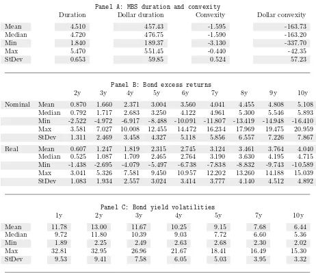
and the average dollar convexity is -163.73 with a standard deviation of 57.23.16 Table
1 presents a summary statistic of all main variables used.
[Insert Table1 and Figure1 here.]
We use the G¨urkaynak, Sack, and Wright (2007, GSW henceforth) zero-coupon
nomi-nal yield data available from the Federal Reserve Board. We use the raw data to calculate
annual Treasury bond excess returns for 2- to 10-year bonds. We also download interest
rate swap data from Bloomberg from which we bootstrap a zero-coupon yield curve.
To calculate real bond excess returns, we use liquidity-adjusted real bond yields (see
D’Amico, Kim, and Wei (2014)).17
We denote the annual return between time t and one year later on a τ-year bond
with price Λτ
t by rτt,t+1y = log Λ τ−1y
t+1y −log Λτt. The annual excess bond return is then
defined as rxτ
t,t+1y = rτt,t+1y −y 1y
t , where y 1y
t = −log Λ 1y
t is the one-year yield. From
the same data, we also construct a tent-shaped factor from forward rates, the Cochrane
and Piazzesi (2005) factor (CP factor, labeled cpt). Real annual excess bond returns are
denoted by rxτ∗ t,t+1y.
Using the GSW yields ranging from one to ten years, we estimate a time-varying
term structure of yield volatility. We sample the data at the monthly frequency and
take monthly log yield changes. We then construct rolling window measures of realized
volatility using a 12-month window which represent the conditional bond yield volatility.
The resulting term structure of unconditional volatility exhibits a hump shape consistent
with the stylized facts reported in Dai and Singleton (2010), with the volatility peak
being at the two-year maturity (see Table 1, Panel C).
Choi, Mueller, and Vedolin (2014) calculate measures of model-free implied bond
market volatilities for a one-month horizon using Treasury futures and options data from
16
Units are expressed in dollars assuming that the portfolio value is equal to the index level in dollars.
17
the Chicago Mercantile Exchange (CME). We use their data for the 30-year Treasury
bond and henceforth label this measure tivt.
From Bloomberg, we also get implied volatility for at-the-money swaptions for
dif-ferent maturities ranging from one to ten years and we fix the tenor to ten years. We
label these volatilities ivτ10y. Further, we collect implied volatilities on 3-month-maturity
swaptions with tenors ranging between 1 and 10 years, denoted by iv3mτ.
As a proxy of illiquidity in bond markets, we use the noise proxy from Hu, Pan,
and Wang (2013), which measures an average yield pricing error from a fitted yield
curve. As a proxy for economic growth we use the three-month moving average of
the Chicago Fed National Activity Index. Negative (positive) values indicate a below
(above) average growth. We also use a measure of inflation proxied by the consensus
estimate of professional forecasts available from Blue Chip Economic Forecasts.
4 Empirical analysis
In this section we study the predictive power of MBS dollar duration and convexity
for bond excess returns (nominal and real) and bond yield volatility. We start with
univariate regressions to document the role of our main explanatory variables. Then,
for robustness and to address a potential omitted variable bias, we also control for other
well-known predictors of bond risk premia and interest rate volatility. We find that not
only MBS duration and convexity remain statistically significant, but also the economic
size of the coefficients stays stable across different specifications.
The start date for volatility regressions is dictated by the availability of the MBS
convexity time series that starts in January 1997. Daily data for TIPS is available from
the Federal Reserve Board website starting in January 1999, which is the start date for
the real bond return regressions. For all other regressions we start in December 1989.
With each estimated coefficient, we report t-statistics adjusted for Newey and West
4.1 Nominal bond risk premia
Hypothesis 1. A regression of bond excess returns on the duration of MBS yields a
positive slope coefficient for all maturities. Moreover, the coefficients are increasing in
bond maturity and remain significant when we control for the level of interest rates.
This hypothesis is derived from Propositions 1 and 2. To test it, we run linear
regressions of annual excess returns on the duration factor. The regression is as follows:
rxτt,t+1y =β τ 0 +β
τ
1durationt+β2τlevelt+ǫτt+1y,
where durationt is MBS dollar duration and levelt is the one-year yield. The univariate
results are depicted in the upper two panels of Figure 2, which plot the estimated slope
coefficients of duration, ˆβτ
1 (upper left panel), and the associated adjusted R2 (upper
right panel). Both univariate and multivariate results are presented in Table 2.
[Insert Figure2 and Table 2 here.]
The univariate regression results indicate that MBS duration is a significant
dictor of bond excess returns across all maturities. In line with the theoretical
pre-diction, the coefficient has a positive sign and is increasing with maturity.18 The
es-timated coefficients are also economically significant, especially for longer maturities.
For example, for any one standard deviation increase in MBS dollar duration, there is a
0.0636×59.85 = 381 (slope coefficient times standard deviation of MBS dollar duration)
18
We can also test whether the estimated slope coefficients are monotonically increasing using the monotonicity test developed by Patton and Timmermann (2010), i.e., we can test whether
H0: ˆβ 10y 1 ≤βˆ
9y
1 ≤ · · · ≤βˆ 2y 1
versus
H1: ˆβ 10y 1 >βˆ
9y
1 >· · ·>βˆ 2y 1 ,
where ˆβτ
1, τ = 2, . . . ,10 years are estimated slope coefficients from an univariate regression from bond
basis point increase in the expected 10-year bond excess returns. Adjusted R2s range
from 7% for the shortest maturity to 23% for the longest maturity.19 To put these effects
into perspective, we can translate the above numbers into the yield space: for any one
standard deviation change in MBS duration, there is a 381/10≈38 basis point increase
in the 10-year yield, assuming that most of the effect on returns happens within the first
year (which we verify in the data below).20
One might suspect that the predictive power of MBS duration could result from its
close relationship to the level of interest rates. Proposition 2, however, allows us to
disentangle the contribution of the two factors. To this end, we include the latter as a
control in our multivariate test. The results presented in Table2indicate that the slope
coefficient on duration remains positive and increasing with maturity, while the slope
coefficient on the level of interest rates is negative and decreasing for longer maturities.
This is in line with our theory, where the level of interest rates is not directly related to
bond risk premia, but helps to predict the mean reversion in duration at longer horizons,
and, thus, its coefficients have the opposite sign.
Finally, we study the persistence of the MBS dollar duration effect on bond risk
premia by varying the horizon of excess bond returns in our predictive regression:
rx10t,ty+h =β0+β1durationt+ǫt+h,
wherehis 3, 6, 12, 24, and 36 months, respectively. We formulate the following
hypoth-esis in line with Proposition 3:
Hypothesis 2. A regression of bond excess returns on the duration of MBS yields
co-efficients that are hump-shaped across horizons, i.e., they are largest for intermediate
horizons.
[Insert Figure 3here.]
19
Our conclusions remain the same when we use interest rate swaps instead of Treasury data, and the duration of the Bank of America US Mortgage Master index (Bloomberg ticker M0A0) instead of Barclays data (see the Online Appendix).
20
The results are presented in Figure3. We find that coefficients increase up to
approx-imately a one-year horizon, but then plateau and decrease, suggesting that the effect
of MBS duration on bond returns is transitory. Our model provides one possible
ex-planation for this: both the mean reversion in interest rates and refinancing activity
contribute to the fast mean reversion in aggregate MBS duration. The short-lived effect
of MBS duration on bond returns could also be explained by the dynamics of arbitrage
capital that, while slow-moving, ultimately flows into fixed income markets to absorb
ad-ditional duration risk.21 While both factors are likely to play a role, Section5presents a
calibration of our model that can quantitatively account for the pattern of multi-horizon
regression coefficients.
4.2 Real bond risk premia
According to our model, the variation in MBS duration should affect the pricing of both
nominal and real bonds. This prediction allows us to differentiate between duration and
factors that are related exclusively to inflation risk. To this end, we test the following
hypothesis based on Propositions 1 and 5:
Hypothesis 3. A regression of real bond excess returns on the duration of MBS yields
a positive slope coefficient that is increasing with maturities. Moreover, real slope
coef-ficients are approximately equal to nominal slope coefcoef-ficients adjusted by the correlation
between real and nominal rates times the ratio of their volatilities.
Univariate results are presented in Figure 2 (middle two panels) and Table 3. We
find that MBS dollar duration significantly predicts real bond excess returns at longer
maturities. For instance, for the 10-year real bond, the estimated coefficient is positive,
highly significant, and implies that any one standard deviation change in MBS dollar
duration leads to a 0.0293 × 68.25 = 199 (regression coefficient times the standard
deviation of MBS dollar duration between 1999 and 2013) basis point change in real
excess returns.
21
The relative magnitude of real and nominal coefficients supports a duration risk
explanation of return predictability. Over our sample period from 1999 to 2013, real
rates are less volatile than nominal rates (σ⋆
σ ≈ 0.72) and the two series exhibit less
than perfect correlation (ρ ≈ 0.87). Accordingly, the effect of duration on real bond
returns is lower. For the 10-year maturity, the ratio of real to nominal coefficients is
199/341 = 0.58, in line with the 0.87×0.72 = 0.62 predicted by our theory.22
[Insert Table3 here.]
4.3 Bond yield volatility
Proposition 4 allows us to formulate the following hypothesis regarding the effect of
MBS convexity on bond yield volatility across maturities:
Hypothesis 4. A regression of conditional yield volatility on the negative convexity of
MBS results in a positive slope coefficient for all maturities. Moreover, the coefficients
are the largest for intermediate maturities, i.e., they have a hump-shaped term structure.
Due to the amplification channel described earlier, we expect a more negative
con-vexity of MBS to result in larger bond yield volatility. To this end, we run the following
univariate regression from conditional bond yield volatility onto MBS convexity:
volτt =β τ
0 +β1τconvexityt+ǫ τ t,
where volτt is the conditional bond yield volatility at time t of a bond with maturity
τ = 1, . . . ,10 years.
The univariate results are presented in the lower two panels of Figure 2 and in
Table 4. In line with our intuition, we find a significant effect from convexity onto bond
22
yield volatility, and the effect is most pronounced for intermediate maturities.23 The
estimated slope coefficients produce the hump-shaped feature similar to the one observed
in the unconditional averages of yield volatility. Adjusted R2s range from 19% for the
shortest maturities, increase to 22% for the two- and three-year maturities, and decrease
again to 14% for longer maturities. Estimated coefficients are not only statistically but
also economically significant: For the two-year maturity, any one standard deviation
change in MBS dollar convexity is associated with a 37 (= 0.0764 (slope coefficient) ×
57.23 (standard deviation of MBS dollar convexity)×2.43 (level of 2-year yield)×√12)
basis point increase in annual bond yield volatility.
[Insert Table4 here.]
An obvious concern with our regression results is that negative convexity could itself
depend on volatility. Note, that it is a priori unclear in which direction volatility affects
convexity as this depends on whether a particular MBS is in-, out-, or at-the-money.24
For an at-the-money MBS, an increase in volatility will lead to an increase in negative
convexity. Discount (i.e., small negative to positive convexity) and premium (negative
convexity) mortgages will in general have a much lower sensitivity to changes in volatility,
and the effect could go in the opposite direction.25
To address causality, we run Granger tests between MBS dollar convexity and
volatil-ity and present the results in Figure4. In the left panel, we plot F-statistics of Granger
causality tests that assess the null hypothesis whether negative convexity does not
Granger cause volatility. On the right panel, we plot the corresponding F-statistics
of the reversed Granger regression, i.e., we test the null hypothesis whether volatility
does not Granger cause negative convexity. We also plot the 10% critical values. We
23
While there are no formal procedures which specifically test for a hump-shape, we can test whether the estimated coefficient on the 2-year bond yield volatility is statistically different from the 3-year volatility. Indeed, the difference, which is 0.0192, has a t-statistic of 2.75 and is hence different from zero. We can then again test for monotonicity between the 3-year and 10-year coefficients. Using the procedure from Patton and Timmermann (2010), we strongly reject the null of no relationship as the p-value is basically zero.
24
This is analogous to the Zomma (sensitivity of an option’s Gamma with respect to changes in the implied volatility) for equity options.
25
note that for standard confidence levels, we can reject the null of no Granger causality
from convexity to volatilities for any maturity. On the other hand, longer-maturity yield
volatility does seem to Granger cause convexity as indicated by the F-statistics.
[Insert Figure 4here.]
4.4 Two MBS investor types: the GSEs and the Federal Reserve
Our paper builds on the premise that fluctuations in MBS duration prompts investors
to adjust their hedging positions, rebalance their portfolios, or, more generally, revise
the required risk premia at which they are willing to hold bonds. While we do not
observe the behavior of all mortgage investors, we can gauge the validity of the duration
channel by looking at market participants with well-defined institutional mandates, and
test whether the change in the composition of MBS ownership over time has an effect
on expected bond returns.
The two GSEs, Fannie Mae and Freddie Mac, play a central role in the US housing
finance system. In addition to their business of issuing and providing credit guarantee
for a large fraction of pass-through MBS, these institutions also retain a significant
portfolio of mortgage loans and MBS. Unlike that of the guaranteed portfolio, all of the
interest rate risk of the retained portfolio lies with the GSEs. Moreover, Fannie Mae
and Freddie Mac see the hedging of this exposure as part of their mandate, including
the part driven by mortgage prepayment.26 Hedging is done through interest rate swaps
under which they trade the fixed-rate interest payments of mortgage loans for
floating-rate interest floating-rate payments that correspond more closely to their short-term borrowing
costs. To hedge prepayment risk, the GSEs issue callable debt and buy swaptions. If
interest rates fall, the GSEs can redeem their callable debt at lower rates, or similarly,
exercise their swaptions. Historically, the GSEs have started hedging during the 1990s
(see Howard (2013)).
26
The top panel of Figure 5 illustrates the relationship between the notional value
of the GSEs’ derivative contracts and MBS duration.27 We note that the value of the
hedging position on average exceeds one trillion USD, and its peaks coincide with the
large drops in MBS duration around 2003 and 2008.
The middle panel of Figure 5 shows the growth of Fannie Mae and Freddie Mac’s
retained portfolio from approximately USD 200bn in the 1990s to almost USD 1.6tr in
2003. The increase in the GSEs’ retained portfolio occurred in parallel with the overall
growth of the MBS and Treasury markets. The bottom panel of Figure 5 presents the
value of the retained portfolio as a share of total outstanding MBS. We note that the
fraction of MBS held by the GSEs is positively associated with the predictive power of
MBS duration on bond excess returns, with both increasing until the mid-2000s and
falling subsequently. While we do not observe the portfolio of other MBS investors
(with an important exception of the Federal Reserve considered below), this evidence
supporting the role of actively hedging GSEs is in line with the MBS duration channel.28
[Insert Figure 5here.]
Whereas the GSEs represent a class of investors who actively manage the interest
rate exposure of their MBS portfolio, the Federal Reserve does not aim to hedge the
duration risk of its MBS holdings. On 7 September 2008 the Federal Housing Finance
Agency (FHFA) together with the Treasury outlined a plan to (i) place both GSEs into
conservatorship and (ii) having the Treasury enter into senior preferred stock purchase
agreements with both firms. The latter require both Fannie Mae and Freddie Mac to
wind down their retained investment portfolio at a rate of at least 10% per year until they
each fall below USD 250bn. This large reduction in the actively hedged GSE portfolios
is partly offset by the increase in Federal Reserve holdings (see Malz, Schaumburg,
Shimonov, and Strzodka (2014)). As of end 2014, the Federal Reserve holds USD 1.7tr
of agency MBS.
27
According to the Financial Accounting Standard (FAS) 133, any firm is required to publish the fair value of derivatives designated as hedging instruments.
28
To study the effect of this shift in MBS ownership from the GSEs to the Federal
Reserve on bond risk premia, we run the following regression:
rxτ
t,t+1y =β τ
0 +β1τdurationt+β2τfed sharet+β3τdurationt×fed sharet+ǫτt,t+1y,
where fed sharet is the Federal Reserve’s share of total MBS holdings. If the effect of
MBS duration is dampened as the Federal Reserve’s share goes up, we would expect the
loading on the interaction term, βτ
3, to be negative.
The results in Table 5 reveal that the coefficient on MBS duration is still highly
significant and increasing with maturity. In line with our intuition that the increased
MBS holdings of the Federal Reserve have weakened the duration channel, we find
a significant and negative coefficient on the interaction term that is increasing with
maturity.
[Insert Table5 here.]
4.5 MBS duration and other predictors of bond returns
In this section we study MBS duration in relation to other predictors of bond returns
proposed by the literature but not included in our model. First, mortgage
refinanc-ing decisions and hence MBS duration could be a function of the information already
contained in the yield curve. We run the following regression:
rx10t,ty+1y =β0+β1durationt+β2levelt+β3slopet+β4curvet+ǫt+1y,
where levelt,slopet and curvet are the first three yield PCs. Table 6 (column 1) reveals
that the economic and statistical significance of the duration factor remains very close
to the results reported in Table 2. In the second column, we control for the Cochrane
and Piazzesi (2005) factor, which is a linear combination of forward rates. Again, we
MBS duration could also be related to the business cycle as empirical evidence shows
that the refinancing incentive of mortgage holders depends on the economic state (see,
e.g., Chen, Michaux, and Roussanov (2013)). Therefore we control for business cycle
measures that have also been shown to have a significant bearing on bond returns,
namely economic growth and inflation.29 We run the following regression:
rx10t,ty+1y =β0+β1durationt+β2inflationt+β3growtht+ǫt+1y.
The results are presented in Table 6 (third column). Again, we find that estimated
coefficients remain very similar to the baseline regression results presented in Table 2.
Finally, the last column presents regression results when including both yield and macro
factors; we find MBS duration to remain highly statistically significant.
We conclude that the predictive power of MBS duration is not subsumed by either
yield or macroeconomic factors and constitutes a separate channel. We also note that
shocks to MBS duration are much more transient than shocks to either first two yield
PCs or macro variables. For example, we find that MBS dollar duration has a half-life of
around 4 months, whereas the level, slope, inflation, and growth factors have a half-life
of 83, 23, 15, and 14 months, respectively.
4.6 MBS convexity, other determinants of yield volatility, and swaption implied
volatil-ity
We now control for additional determinants of yield volatility that have been documented
in the literature. For example, it is well-known that volatility tends to increase in
periods of high illiquidity (see, e.g., Hu, Pan, and Wang (2013)). In our multivariate
specification, we therefore add a proxy for illiquidity and a proxy of fixed-income implied
volatility, similar to the VIX in equity markets. We run the following regression from
conditional bond yield volatility onto MBS dollar convexity and a set of other predictors:
volτt =βτ
0 +β1τconvexityt+β2τilliqt+β3τtivt+ǫτt,
29
where volτ
t is the conditional bond yield volatility at time t of a bond with maturity
τ = 1, . . . ,10 years, illiqt is the illiquidity factor at time t, and tivt is the
Treasury-implied volatility at timet. Results are reported in Table7(panel A). We find that when
we add illiquidity and tiv to the regression, convexity still remains highly statistically
significant. The estimated coefficients in the bond yield volatility regressions reveal that
the effect is largest for the intermediate maturity of two years as indicated by the size
of the coefficient. All three factors together explain between 27% and 43% of the time
variation in bond yield volatility across different maturities.
[Insert Tables 7here.]
As hedging can potentially take place both in the bond and in the fixed-income
derivatives market, we also test the impact of MBS dollar convexity on measures of
implied volatility from swaptions. For example, Wooldridge (2001) notes that
non-government securities were routinely hedged in the Treasury market until the financial
crisis of 1998 when investors started hedging their interest rate exposure in the swaptions
market.
Table 7, panels B and C present estimated coefficients when regressing either implied
volatility ofτ-maturity swaptions written on the 10-year swap rate (panel B) or implied
volatility of 3-month swaptions written onτ-maturity swap rates (panel C). We find that
the effect is stronger for shorter maturities and tenors, and all coefficients are positive
and highly significant.
5 Calibration
In this section we calibrate our model to test its quantitative performance.
5.1 Estimated and calibrated parameters
of the monthly series of MBS dollar duration as the associated R2 is 83%. In order to
fully characterize the theoretical effect of MBS duration and convexity on bond returns
and yield volatility, we set the risk aversion of financial institutions to α = 88. This
value allows the model to match the R2 of the predictive regression of 10-year nominal
bond excess returns on duration reported in Table 2. Note that α is the coefficient
of absolute risk aversion. In order to interpret this value, we multiply it by financial
institutions’ wealth to obtain a coefficient of relative risk aversion. In a setting similar to
ours, Greenwood and Vayanos (2014) use financial institutions’ capital to GDP ratio of
13.3%. Because we use the dollar duration of the MBS index to calibrate the model and
the average value of the index itself is standardized to one dollar, we also need to adjust
for the size of the MBS market relative to GDP. Between 1997 and 2012 the average
value of outstanding mortgage-related debt was equal to 53% of the GDP. This implies
a coefficient of relative risk aversion of approximately 22≈88×13.3%/53%.
We summarize all calibrated parameter values in Table 8.
[Insert Table8 here.]
5.2 Return predictability and volatility
The calibrated model provides a benchmark for the empirical results in Section 4. The
two top panels of Figure6report the term structure of theoreticalβτ,h andβτ,h∗together
with our empirical estimates. The coefficients implied by the model are within the 95%
confidence intervals for maturities up to 8 years, but it underpredicts them at the long
end.
The lower left panel of Figure 6 reports the theoretical slope coefficients β10y,h for
different return horizons. In line with our empirical estimates, the coefficients increase
steeply up to approximately one year before they plateau and then decrease. This
suggests that the mean reversion in aggregate MBS dollar duration is enough to account
for the transitory nature of its effect on bond returns.
The lower right panel of Figure 6 reports the total change in yield volatility across
model implies a 48 basis point increase in the two-year yield volatility relative to the
case where the negative convexity channel is shut down. This can be compared to the
estimated 131 basis point change in the two-year yield volatility that would result from
a 2.9-standard-deviation shock bringing convexity from its average value to zero.30 In
line with our empirical findings, the calibrated model implies that the effect of negative
convexity is hump-shaped and strongest for maturities around two and three years.
[Insert Figure 6here.]
5.3 MBS duration and the cross-section of yields
We also look at the ability of the calibrated model to match additional stylized facts
regarding the information in MBS duration and its relation to the information encoded
in yields. Table6reveals that the predictive power of our duration factor remains largely
unaffected when we control for the first three principal components of yields. Moreover,
regressing duration on these yield factors results in an R2 of a mere 22%.
While our stylized model is not designed to address the possibility that MBS duration
is unspanned, the calibration exercise nevertheless speaks to the empirical facts. In the
calibrated model the short rate factor explains over 96% of the variation in yields across
maturities, but only around 7% of the variation in MBS duration and only around 1% of
the one-year excess return on the 10-year bond. At the same time, duration accounts for
all the return predictability and explains the same proportion of 10-year bond returns
(R2 = 24%) in the model as in the data. In other words, the factor that accounts for all
the predictive power is not strongly related to the factor that accounts for a dominant
fraction of the cross sectional variation in yields.
30
6 Conclusion
In this paper we study both theoretically and empirically the feedback from the
fluc-tuations of aggregate MBS risk onto the yield curve. Our model makes the following
predictions. First, MBS duration increases both nominal and real bond excess returns
and the effect is strongest for longer maturities. Second, the predictive power of MBS
duration for bond excess returns is transient. Third, MBS convexity positively affects
bond yield volatilities and the relationship is hump-shaped across maturities.
We test these predictions in the data and find strong support. In particular, any
one standard deviation change in MBS duration increases expected annual 10-year bond
returns by 381 basis points, while real bond returns increase by 199 basis points. Since
the effect of MBS duration on expected returns is transient in nature and becomes
insignificant for a horizon beyond one year, this translates to a rise in nominal (real)
10-year yields of 38 (20) basis points today. Our results are comparable in magnitude to the
impact of the recent Quantitative Easing programs implemented by the Federal Reserve:
the cumulative effect of all large-scale asset purchases taken together is estimated to
be between 80 and 120 basis points (see Stein (2012)). For volatility, we find that a
one standard deviation change in MBS convexity, changes 2-year bond yield volatility
by 37 basis points. Finally, we calibrate our model to the data and find that our
model successfully produces effects which are quantitatively in line with their empirical