University of Warwick institutional repository: http://go.warwick.ac.uk/wrap
A Thesis Submitted for the Degree of PhD at the University of Warwick
http://go.warwick.ac.uk/wrap/63944
This thesis is made available online and is protected by original copyright. Please scroll down to view the document itself.
M A
E
G
NS I
T A T MOLEM
U N
IV
ER
SITAS WARWICEN
SIS
Simple Collision Operators for Direct
Vlasov Solvers
by
Daniel Fletcher
Thesis
Submitted to the University of Warwick
for the degree of
Doctor of Philosophy
Department of Physics
Contents
Acknowledgments iv
Declarations v
Abstract vi
Chapter 1 Introduction 1
1.1 Thesis Overview . . . 1
1.2 Fusion Energy Overview . . . 2
1.2.1 Ignition and Breakeven . . . 2
1.3 Inertial Confinement . . . 4
1.3.1 Overview . . . 4
1.3.2 Fast Ignition . . . 8
1.3.3 Shock Ignition . . . 10
1.4 Plasma Physics Overview . . . 10
1.4.1 Kinetic Theory and Vlasov’s Equation . . . 10
1.5 Collisions in an Ionised Gas . . . 13
1.5.1 Coulomb Collisions . . . 13
1.5.2 Collision Operators . . . 17
1.5.3 Transport Coefficients . . . 18
1.6 Collisional and Collisionless aspects of Laser-Plasma physics . . 20
1.7 Summary . . . 23
Chapter 2 Computer Simulation of The Vlasov-Maxwell System 24 2.1 Introduction . . . 24
2.2 The Vlasov-Maxwell System . . . 28
2.3 Numerical Schemes and the VALIS code . . . 29
2.3.2 Updating the Distribution Function . . . 31
2.3.3 Updating the Fields . . . 37
2.4 Normalisation . . . 40
2.5 Parallelisation Using MPI . . . 41
2.5.1 Domain Decomposition . . . 41
2.5.2 Synchronisation and Non-Blocking Communication . . . 41
2.5.3 File IO . . . 42
2.5.4 Boundary Conditions . . . 42
2.6 Numerical Tests . . . 43
2.6.1 Landau Damping . . . 43
2.7 Summary . . . 46
Chapter 3 A Phenomenological Approach to Collisions: the Krook Model 47 3.1 Introduction . . . 47
3.2 Implementation . . . 49
3.2.1 Electron-Ion Collisions . . . 52
3.2.2 Relativistic Collisions . . . 53
3.2.3 Quick Collisions . . . 54
3.3 Collision Frequencies . . . 54
3.4 Heat Flux Normalisation . . . 57
3.5 Implementation Notes and Optimisation . . . 58
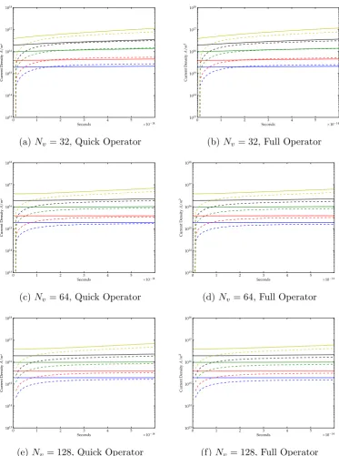
3.6 Transport Test Results . . . 59
3.6.1 Electrical Conductivity . . . 59
3.6.2 Thermal Conductivity and Non-local Transport . . . 62
3.7 Discussion . . . 72
Chapter 4 Using the Krook Operator to Model Laser Heating 73 4.1 Introduction . . . 73
4.2 Implementation . . . 73
4.3 Using Separate Distributions . . . 76
4.4 Summary . . . 80
Chapter 5 Model Fokker-Planck Operators 82 5.1 Introduction . . . 82
5.2 Electron-Ion Collisions . . . 84
5.3.1 Approach to Equilibrium . . . 85
5.3.2 Collisional Heating and Electrical Conductivity . . . 92
5.4 Summary . . . 94
Chapter 6 Fast Electron Transport and Return Currents 95 6.1 Introduction . . . 95
6.2 Simulation . . . 95
6.3 Results . . . 97
Acknowledgments
I’d like to thank my parents for their continuing support and belief in me
throughout my studies. I’d also like to thank my supervisor, Tony for helpful
Declarations
All work and results presented in this thesis were produced by myself except
Abstract
Existing codes for directly solving for the particle distribution function
in laser plasma interaction studies either assume a collisionless plasma or solve
for the full Fokker-Planck collision term. The former approach is the basis of
an existing code at Warwick (VALIS). The latter approach is computationally
expensive and often relies on a spherical harmonic expansion of the
distribu-tion funcdistribu-tion, making the implementadistribu-tion of a laser driver difficult. Here the
existing collisionless code is extended by including reduced collision operators
based on both the Krook and Fokker-Planck operator. The formulation of
a fully conservative velocity-dependent Krook operator that shows agreement
classical transport co-efficients in the regimes they are valid. The accuracy of
the operator is shown to be improved using a normalisation method to ensure
the Krook model yields the same heat flux as the Fokker-Planck model. The
Krook model is also shown to be in agreement with full Vlasov-Fokker-Planck
simulations of non-local transport. Two forms of a model Fokker-Planck
Chapter 1
Introduction
1.1
Thesis Overview
precludes resolution of electrostatic instabilities. The Vlasov-Maxwell-Krook code here employs an explicit field algorithm which can resolve these features.
1.2
Fusion Energy Overview
The concept of nuclear fusion as a source of energy began with the discovery of the mass-energy equivalence arising from the theory of special relativity developed by Einstein in 1905. The consequences of this relation for atomic physics were revealed by Aston in 1920 when his accurate mass spectrometry revealed the mass of four hydrogen atoms was greater than the mass of one helium atom. This discovery led to Eddington proposing that this change in mass due to the fusion process was the source of energy production in stars. Studies of nuclear physics in the 1920’s and 30’s allowed Bethe [2,3] to describe a sequence of thermonuclear reactions that could occur under the conditions at the centre of a star, known as the carbon cycle. This cycle is dominant in stars
with core temperatures above 109K. In stars with cooler core temperatures
however, such as our Sun, the proton-proton cycle is more common,
H11+H11→D12+e++ν (1.44M eV)
D11+H11→He32+γ (5.49M eV)
He32+He32→He24+ 2H12 (12.86M eV)
Where e+, ν and γ denote positrons, neutrinos and gamma rays
re-spectively and the numbers in brackets denote the energy released by each reaction.
1.2.1
Ignition and Breakeven
with equal number densities, nD =nT =n, the power generated by a nuclear fusion reactor per unit volume is given by,
Pf us =
1
4n
2
hσvi∆E
wherehσviis the reaction rate which is the reaction rate derived from the
colli-sional cross section,σ and the relative particle velocities. For a D-T plasma at
10KeV,hσvi ∼ 1.1×10⁻²²m3s−1[5], and ∆E for the D-T reaction is 17.6M eV,
thus the power generated per unit volume,Pf us = 7.7×10⁻³⁵n2W m−3. Of the
energy released in the D-T fusion reaction, only 20% is in the form of kinetic energy to alpha particles which are able to heat the plasma to sustain the
nuclear reactions. The power available from the alpha particles,Pα = 0.2Pf us.
The rest of the energy is carried by the neutrons which pass through the plasma into the walls of the reactor. The rate of other energy losses must also be taken into account such as radiative losses through bremsstrahlung and heat loss to
the reactor wall. The energy confinement time τE is a measure of the rate of
these losses. This is the ratio of the plasma energy density to the rate at which
energy is lost,τE=W/Ploss where W = 3nkBT. The ignition criteria requires
the power generated to be at least equal to the power lost from the plasma,
Pα ≥Ploss
substituting in the values derived earlier,
1
4n
2
hσvi∆Eα =
3nkBT
τE
which can be written as,
nτE ≥
12
Eα
kBT
hσvi
It’s useful to write an expression for this criteria as a triple product,
neT τE ≥C
where C is a constant depending on the cross section of the nuclear reaction
in question. For the Deuterium-Tritium reaction, C = 1021keV.s/m3.
must be confined through alternative means. Magnetic confinement devices utilise the charged particle nature of a plasma to contain along magnetic field lines. A Tokamak confines the plasma in a toroidal chamber using the combi-nation of toroidal and poloidal field lines. Since magnetic confinement devices contain the plasma for long periods of time, the energy carried by the neutrons is able to be converted into electricity by the reactor which can in turn be used to heat the plasma. In this case the Lawson criteria refers to breakeven, rather than ignition and requires,
Pα+ηPn=
3nkBT
τE
whereηis the efficiency of conversion from neutron energy to a heating
mech-anism and Pn is the power supplied by the neutrons. Since the total energy
carried by the neutrons is five times that of the alpha particles, this can be written as
Pα =
3nkBT
τE
. 1
1 + 5η
Breakeven can therefore be met with a lowerPα than is required for ignition.
The ITER tokamak device currently under construction in the south of France aims to reach breakeven after full deuterium-tritium operation begins in 2027 [6], with an ultimate aim of producing 10 times as much power as it consumes.
1.3
Inertial Confinement
1.3.1
Overview
Inertial Confinement Fusion in contrast to Magnetic Confinement Fusion at-tempts to reach ignition by compressing the plasma to far higher densities so that the Lawson criterion can be satisfied with a confinement time many orders
of magnitude smaller. The energy confinement time, τE in this case is simply
due to the inertia of the D-T fuel rather than external magnetic fields. For the D-T reaction the triple product can be written
A sphere of fuel is heated to 108K and expands at the thermal velocity,
vth ∼
kBT
¯ m
∼6×10⁵ms−1
where ¯m is (mD+mT)/2. If the sphere expands to double the volume then
the radius is increased by 1
4. Estimating the energy confinement time as,
τE =
R
4vth
equation 1.1 can be written as
nR≥7.2×1026
or multiplying by ¯m to give the mass density, ρ,
ρR ≥0.3g.cm−2
The burn fraction Φb, in other words the fraction of the DT fuel that can be
expected to fuse before it flies apart can be show to be [7],
Φb'
ρR
ρR+ 6
and fusion energy output for this fraction can be calculated to be
Ef us = 3.3×10¹¹Mb
where Mb is the DT mass burned. Assuming Φb = 1/3 and setting an upper
limit of fusion energy output to ensure the survival of the reactor at Ef us =
10M J (2.5kg TNT). The corresponding D-T fuel mass, M = 10−4g. The mass
of a spherical fuel capsule can be written,
M = 4π
3
(ρR)3
ρ2
and since ρR = 3g/cm2 is needed, compression up to ρ = 103g/cm3 is
re-quired to achieve ignition. For liquid density D-T fuel, ρ= 0.21g/cm3 so this
Figure 1.1: Fuel Capsule Prototype at the National Ignition Facility [8]
Inertial confinement fusion refers to a range of device designs which use lasers to heat and compress a fuel target. The largest inertial confinement experiment currently in operation is the National Ignition Facility(NIF) at Lawrence Livermore National Laboratory. The Laser driver at NIF is able to generate a 500 Terawatts with a peak energy of 1.8 Megajoules with a tem-poral pulse length of 10-20 nanoseconds [9]. The target capsule(figure 1.1 is comprised of an outer ablator shell made of a low Z material such as beryllium or a high density carbon and an inner fuel shell of deuterium-tritium ice which surrounds a core of DT gas. The core is a lower density to reduce its pressure therefore reduce the work required for compression. Figure 1.2 outlines the stages of an inertial confinement experiment. Initially the surface of the spher-ical target is irradiated by the laser and is rapidly heated. The hot outer shell rapidly rapidly expands reaching a pressure of around 100Mbar generating an implosion wave through the rocket effect. For ignition this implosion velocity,
uimp needs to be greater than 300−400km/s. The imploding fuel reaches the
highest temperature at the centre of the target where ignition occurs. The thermonuclear burn then propagates from the centre of the target through the surrounding fuel.
Figure 1.2: Stages of inertial confinement fusion [10]
at the cost of reduced coupling efficiency between the laser energy input and the fuel capsule.
Figure 1.3: Overview of an indirect drive inertial confinement experiment. Image reproduced from Lawrence Livermore National Laboratory [11]
The hot spot at the centre of the compressed fuel capsule of radiusRh is
typically much smaller than the initial capsule radius. The convergence ratio,
Cr =R0/Rh ∼30−40 [12]. Deformations in the hotspot, δRh/Rh are related
to implosion velocity asymmetry. The difference in radius, after an implosion
timetimp
R0−Rh =uimptimp
esti-mated,
δRh
Rh ∼
R0
Rh −
1
δuimp
uimp
the asymmetry in implosion velocity is due to pressure non-uniformity which itself is due to the asymmetry in target irradiation,
δuimp
uimp ∼
δpa
pa ∼
2 3
δI I
where growth of hydrodynamic instabilities due to pressure non-uniformity has
been neglected. With these assumptions one still requiresδI (3/2)(Rh/R0).
1.3.2
Fast Ignition
Fast ignition is an ignition scheme where a hot spot is created after the fuel capsule has already begun imploding. In conventional fast ignition(see figure
1.4), an ultra-intense(∼ 1020W/cm2) laser pulse is then fired which generates
a beam of fast electrons around the critical density which produce a hot spot when they are stopped when they meet the compressed plasma. Such a scheme relaxes the symmetry requirements needed to generate a central hotspot re-quired by conventional ICF schemes. The reduction in rere-quired laser energy and hydrodynamic requirements of the fuel capsule mean that fast ignition has the potential to produce greater gain. Numerous fast ignition schemes exist and are summarised in figure 1.6
Laser
Fast electron generation
Imploding fuel
Figure 1.4: Conventional Fast ignition
alleviate this problem in conventional fast ignition the ultra-intense igniter
beam is preceded by a lower power, hole boring pulse(∼ 1018W/cm2). This
then allows the igniter pulse to propagate uninhibited through the tunnel in the coronal plasma. Cone guided fast ignition uses a gold cone inserted into the side of the target. The gold cone maintains a vacuum during the implosion phase through which the igniter pulse can propagate. Fast electrons are generated when the igniter pulse hits the cone tip.
Imploding fuel Guiding Cone
Laser
Figure 1.5: Cone Guided Fast ignition
1.3.3
Shock Ignition
Shock ignition [14] is another scheme which attempts to reach ignition through the collision between shocks. A central hotspot is created when a second, spherical symmetric ignitor shock, generated by a spike in laser energy collides with the reflected initial shock.
1.4
Plasma Physics Overview
1.4.1
Kinetic Theory and Vlasov’s Equation
Rather than considering the overall bulk evolution of the plasma, kinetic theory instead considers the motion of each individual particle. The position and
velocity of a single particle at a time t can be defined as its density function
over phase space,
N(x,v, t) =δ[x−X1(t)]δ[v−V1(t)]
Wherexandvare Eulerian co-ordinates in six dimensional phase space
as x = (x, y, z) and v = (vx,vy,vz). X1 and V1 are the Lagrangian
co-ordinates of the particle itself andδ is the Dirac delta function. If the particle
exists at X1 = x and V1 = v the density function equals infinity there and
zero everywhere else.
To get a complete description of all the particles of speciessthe density
function must sum over N0 the number density of the particles,
Ns(r,v, t) =
N0 X
i=1
δ[x−Xi(t)]δ[v−Vi(t)]
At any timetthe density of particles integrated over phase space is equal to the
number of particles in the system. This follows from 1.4.1 due to the property of the Dirac delta,
Z ∞
−∞
δ(x)dx= 1
The total density is then given by the sum over each species, e.g. electrons and ions:
N(x,v, t) =X
e,i
Since derivative of the position is simply the velocity, it follows that if the
position and velocity of a particle is known at a timet then we know them at
all previous and later times. So
˙
Xi(t) =Vi(t) (1.2)
where the overdot denotes the derivative with respect to time. The change of velocity with respect to time is given by the acceleration due to the Lorentz force,
Fi(t) = msV˙i(t) =qsEm[Xi(t), t] +
qs
cVi(t)×B
m[
Xi(t), t] (1.3)
Where the superscript m denotes the fields generated self-consistently by the
point particles. These fields satisfy Maxwell’s equations:
∇.Em(x, t) = ρ
m(x, t)
0
∇.Bm(x, t) = 0
∇ ×Em(x, t) =−∂B
m(x, t)
∂t
∇ ×Bm(x, t) =µ0Jm(x, t) +
1
c2
∂Em(x, t)
∂t
Where the microscopic charge density and current are defined as:
ρm(x, t) =X
s qs
Z
Ns(x,v, t)dv
Jm(x, t) =X s
qs Z
vNs(x,v, t)dv
DifferentiatingNs with respect to time:
∂Ns ∂t = N0 X i=1 ∂
∂tδ(x−Xi)
δ(v−Vi) +
N0 X
i=1
δ(x−Xi)
∂
∂tδ(v−Vi)
(1.4)
using the chain rule, for example ∂
∂t(x−Xi) = − dXi
dt . ∂
1.2 and 1.3, equation 1.4 becomes: ∂Ns ∂t = N0 X i=1 =− N0 X i=1
Vi.∇xδ[x−Xi(t)]δ[v−Vi(t)]− N0 X
i=1
Fi.∇xδ[x−Xi(t)]δ[v−Vi(t)]
(1.5)
Using the relation g(x)δ(x−x0) = g(x0)δ(x−x0), inserting equation 1.4.1
yields the Klimontovich equation:
∂Ns
∂t +v.∇Ns+
qs
ms
(Em+v×Bm).∇vNs= 0 (1.6)
We have obtained a set of equations which in terms of classical mechan-ics, completely determines the system. The Klimontovich equation however involves the summation over every single particle in the system. While being an exact description of the system, the Klimontovich equation is too complex to perform any meaningful calculations with and useful only as a starting point from which to derive average properties.
A more useful measure of the system is to consider a smooth function
that yields the number of particles found in a volume ∆x∆v of phase space.
Suppose we are interested in long range electric and magnetic fields that extend over ranges much larger than the inter-particle spacing. A volume of
configu-ration space ∆x centred about x can be chosen. The number of particles in
that volume with velocities falling within a range v+ ∆v can be normalised
and the result is the distribution function, fs(x,v, t). The evolution of this
function with time will be in good agreement with the ensemble average of the density function. The spikey effects due to the discrete nature of the particles can be decoupled using the definitions:
Ns(x,v, t) =fs(x,v, t) +δfs(x,v, t)
Em(x,v, t) =E(x,v, t) +δE(x,v, t)
Bm(x,v, t) =B(x,v, t) +δB(x,v, t)
Where E and B are the ensemble averages of Em and Bm respectively.
In-serting these into the Klimontovich equation (1.6) gives the plasma kinetic equation:
∂fs
∂t +v.∇xfs+
qs
ms
(E+v×B).∇vfs =−
qs
msh
(δE+v
The terms on the left of equation 1.7 vary smoothly in phase space containing collective effects, while the terms on the right is the ensemble average of spiky terms that arise due collisions and individual particle correlations. Dropping these terms yields Vlasov’s equation:
∂fs
∂t +v.∇fs+
qs
ms
(E+v×B).∇vfs= 0 (1.8)
For a relativistic plasma, define u = vγ where γ is the Lorentz factor
which can be defined in terms of u,
γ =
r
1 +|u|
2
c2 .
Defining γ this helps avoid divide by zero problems that could occur when γ
is defined the usual way.
Vlasov’s equation for a relativistic plasma is then:
∂fs
∂t +
u
γ.∇fs+
qs
ms
(E+ u
γ ×B).∇vfs= 0 (1.9)
The Vlasov equation, coupled with Maxwell’s equations describes the evolution of the particle distribution function forced by self-consistent, ensem-ble averaged fields. While this model ignores individual particle interactions it will be shown that it has applicability to a range of astrophysical and labora-tory plasmas.
1.5
Collisions in an Ionised Gas
1.5.1
Coulomb Collisions
Collisions between neutral species are characterised by close range, large angle deflections as particles enter a proximity of the order of the atomic radius of each other. For these collisions the collision frequency is simply the average number of interactions between particles per unit time. In an ionised gas a particle can feel the influence of another particle through the Coulomb force over a much larger distance. The Coulomb force is an inverse square force given in SI units by:
F = q1q2
4π0r2
therefore while being much more common, interactions between particles in a
Figure 1.7: Typical test particle trajectories in a neutral fluid(left) and an ionised fluid(right). The collision time for a neutral gas is the time between collisions while in a plasma the collision time is defined as the time taken for
the electron to be deflected through 90◦due to the Coulomb forces from other
particles
plasma result in the test particles only being deflected through a small angle. An illustration of collisions in a neutral fluid and a plasma are shown in figure 1.7.
To quantify these kind of collisions we will begin by considering binary Coulomb collisions between only two particles, in this case an electron encoun-tering an ion. The geometry of this situation is illustrated in figure 1.8.
The electron has an initial velocity v0, while the ion is heavier and
moves much more slowly than the electron in thermodynamic equilibrium, so here the ion will be treated as if it is infinitely heavy and thus its trajectory is unchanged by the encounter. The encounter between the electron and ion can
be characterised by the impact parameterb, which is the proximity the
parti-cles would have achieved had the electron not been deflected by their coulomb interaction. The velocity gained by the electron in the direction perpendicular to its unperturbed trajectory can be approximated by the integral of the
per-pendicular Coulomb forces(F⊥) on the electron travelling in a straight line at
a distanceb from the ion over time.
mv⊥ =
Z ∞
−∞
i
eb
q0,m0
e t=0
q,m
θ(t) r(t) v0
Figure 1.8: Schematic of a single Coulomb encounter
The scattering angle from a single encounter is assumed to be small such that
v⊥ v0so value of F⊥ can be approximated using the electron’s unperturbed
trajectory, the dotted line in figure 1.8. Using Coulomb’s law,
F⊥=
qq0
4π0r2
sinθe (1.11)
the Coulomb force on the electron can be approximated by assuming it travels
on an unperturbed trajectory thusb=rsinθe and
F⊥ =
qq0
4π0b2
sin3θe (1.12)
The total perpendicular velocity gained by the electron over all time is then, from equation 1.10
v⊥ =
qq0
4π0mb2
Z ∞
−∞
sin3θdt (1.13)
The electron’s position along the dotted line,x=v0t and relates to θ through
x=−rcosθ and usingb=rsinθ,
−bcosθ
sinθ =v0t
so
dt= p
v0
dθ
Using equation 1.13
v⊥ =
qq0
mv0b
Z π
0
sinθdθ
= 2qq0
mv0b
(1.15)
An impact parameter that causes the electron to gain perpendicular
velocity equal to its parallel velocity, v⊥ = v0, i.e. an impact parameter that
causes a deflection ofπ/4 radians can be defined:
b0≡
2qq0
mv2
0
(1.16)
Therefore each b≤ b0 will lead to a large-angle deflection. The cross section
for large-angle scattering by a single particle is given by πb20. The frequency
of these large-angle scatterings for an electron travelling through a medium of background particles is then:
νL =πn0v0b20=
4πn0q2q20
m2v3
0
As it travels through the plasma however, the electron is experiencing many
more small angle deflections with an impact parameterbb0. The maximum
impact parameter that causes a deflection can be set to the Debye length, since after this length charges are screened by particle motions. The frequency in
which many of these small angle collisions lead to a deflection through π/4
radians can be derived by integrating over the range of impact parameters
fromb0to the Debye length(see, for example [15]). This gives the frequency of
deflections through π/4 radians due to many small-angle collisions, or simply
the collision frequency:
νc=
8πn0q2q02lnΛ
m2
ev03
(1.17)
1.5.2
Collision Operators
To include the effect collisions of the type described above on the distribution function described in section 1.4.1, terms must be added to the right hand side of Vlasov’s equation:
∂fs
∂t +v.∇fs+
qs
ms
(E+v×B).∇vfs=
∂f ∂t c (1.18)
Where the term (∂f /∂t)c is the rate of change of the distribution function due
to collisions.
The Fokker-Planck Equation
For many years the Boltzmann collision integral was used for the collision term. This operator, being derived for a neutral gas assumed collisions were dominated by binary, short range interactions. This is not the case for in an ionised gas where collisions are dominated by weak, long-range interac-tions. The Fokker-Planck form of the collision operator was described by Chan-drasekhar [16] by assuming that the motion of a particle undergoing Brownian motion is a Markov process then reducing it to a partial differential equation. It was then formulated for an inverse square force by Rosenbluth, MacDonald and Judd [17] for an arbitrary distribution function in terms of potentials in velocity space in the form:
1 Γ ∂fa ∂t =− ∂ ∂v fa ∂ha ∂v +1 2 ∂2
∂v∂v
fa
∂2g
∂v∂v
The potentials are defined as:
∇2vha =
X
b
ma+mb
mb
fb(v)
and
∇4
vg =−8π X
b
fb(v)
and Γ = 4πq2aqb2lnΛ/ms. This equation describes the change in the distribution
of species a colliding with speciesb.
Bhatnagar-Gross-Krook
The Bhatnagar-Gross-Krook [18] model ignores the complex dynamics of particle-particle interactions and simply models the relaxation to an equilibrium, Maxwellian velocity distribution due to collisions. The operator is given by:
∂f
∂t
=−ν(f −f0) (1.19)
whereνis a collision frequency independent of velocity. The parameters
of the Maxwellian distribution,f0are chosen by taking moments off such that
f0 has the same density, momentum and energy. Collisions between differing
species can also be included in this model in a conservative way [19].
This model can be improved through the use of a velocity dependent collision frequency. However this is not guaranteed to conserve momentum or
energy due to thef0now being applied tof at differing rates in velocity space,
particularly iff is far from equilibrium.
A method for implementing a Krook type collision operator with a ve-locity dependent collision frequency that is conservative will be described and its accuracy in laser-plasma regimes will be assessed in chapter 3.
1.5.3
Transport Coefficients
Since the electrons have a much smaller mass than the ions, they have higher typical speeds when the plasma is in thermal equilibrium. Because of their lower inertia, they are much more easily accelerated by external forces and as such are chiefly responsible for the transport of charge and energy through the plasma. The inclusion of collisions mean particles no longer travel uninhibited at their thermal velocity. The current and thermal flux can be written as [20]
J =σE+α∇T
q =−κ∇T −βE
Where the coefficients, κ and σ are the thermal and electrical conductivities
respectively andα and β are thermoelectric transport coefficients.
equi-librium such that,
f0=fm=n
m
2πkbT
3/2
e−mv2/2kbT
is perturbed by a weak and uniform electric field. This perturbs the plasma
such thatf =f0+f1. Equation 1.18 with the Bhatnagar-Gross-Krook collision
term with a collision frequency independent of velocity,νc, then reduces to
ZeE
m .
∂f0
∂v =−νcf1 (1.20)
From Ohm’s law,σE =j and j can be computed by integrating the
distribu-tion funcdistribu-tion and since the equilibrium distribudistribu-tionf0 has no net current,
j =Ze Z
vf1dv (1.21)
Integrating over velocity space and multiplying byZev, equation 1.20 becomes
νcj =
Z2e2
kbT
E. Z
vvfMdv (1.22)
In 1D, where E = (Ex,0,0) and so J = (Jx,0,0). From equations 1.21 and
1.22 the electrical conductivity is obtained:
σ= nZ
2e2
mνc
(1.23)
The equilibrium distribution function for a plasma inhomogenous in space is
f0(x) =n(x)
m
2πkbT(x)
3/2
e−mv2/2kBT
The steady state, force-free solution of equation 1.18
∂f0
∂x =−νcf1 (1.24)
For the thermal conductivity, assume constant pressure,
so equation 1.24 becomes
f0v.∇T
mv2
2kbT2 −
5
2T
=−νcf1 (1.25)
and the heat flux is given by
q = 1
2m
Z
v2vf1dv
multiplying equation 1.25 by 1
2mv
2v,
νcq =
5m
4T
Z
v2vv.∇T f0dv−
m2
4kbT2
Z
v4vv.∇T f0dv
SinceT =R
12mv2f dv
q =−κ∇T (1.26)
Where the thermal conductivity, κ= 5nk2bT
2mνc. For derivation using the velocity
dependent form of the BGK collision operator see Struchtrup [21].
1.6
Collisional and Collisionless aspects of
Laser-Plasma physics
In certain scenarios the collision time can be much longer than other timescales of interest.
The ratio of the collision frequency to the plasma frequency,
νc
ωpe
where the collision frequency due to Spitzer [22] can be written
νc≈
nZ2e4
2π2
0m2ev03
lnΛ
and taking v0 to be the thermal velocity ∼
p
kBTe/me is then,
νc
ωpe
= lnΛ
2πλ3D =
2lnΛ
Plasma ne(m−3) T(K) ND νc/ωpe
Solar Core 1032 107 1 10−2
Ionosphere 1012 103 105 10−5
Tokamak 1020 108 108 10−7
Solar Wind 106 105 1011 10−11
Interstellar Medium 105 104 1015 10−15
ICF 1022
−1032 105
−109 1
−106 10−5
−1
Table 1.1: Typical Parameters of Laboratory and Astrophysical Plasmas
thus the importance of collisions is inversely proportional toND, the number
of particles in a Debye sphere,
ND=n
4
3πλ
3 D
∝ T
3/2
n1/2
.
For hot and tenuous plasmas ND becomes large such that the collision
fre-quency is much smaller than the plasma frefre-quency. Parameters for a few example plasmas are given in the table 1.1.
While these are approximate values, they give an idea of how the col-lisionality varies with density and temperature. The solar core is hot and dense. Confined by gravity, inter-particle encounters are common. Fusion of hydrogen to helium generates the Sun’s energy. The ionosphere is part of the Earth’s upper atmosphere, where particles are ionised by energetic particles and radiation from the Sun. The density here is low but so is the tempera-ture, so large angle Coulomb deflections are more common. In a Tokamak the plasma is confined along helical field lines. Generally interactions with the EM fields are more important than inter-particle interactions, but collisions are important in understanding the transport of particles across field lines. The solar wind and interstellar medium are very sparse and may be assumed to be collisionless. Inertial confinement experiments range over a wide range of parameters. In an indirect drive scenario, the pre-plasma at the entrance to
the Hohlraum has a ratio νc/ωpe ∼ 10−5 while in the ablator shell this can
be around 10−1−10−2 [23]. An overview of the physics of a high power laser
interacting with matter is illustrated in figure 1.9
Figure 1.9: Summary of the physics of a high power laser hitting a target. Reproduced from Thomas et al. [23]
laser pulse interacts with matter and some characteristics of the plasma in each region. The region on the left corresponds to the region of ablated plasma. Here the plama is hot and tenuous and such that the plasma frequency is much greater than the typical collision frequency. For most studies in this region collisions may be neglected and the plasma is well described by the Vlasov equation. The next region covers the area where either the laser interacts with the plasma in direct drive and laser driven fast ignition schemes, or x-rays radiated from the inside of a hohlraum in indirect drive schemes. Modelling this region requires a method which is able to capture the coupling of laser energy to fast electron energy. This coupling however is still not fully understood with efficiencies derived from numerical and experimental work ranging from 10% up to 90% [24].
The region on the right of figure 1.9 is where the energetic particles propagating ahead of the heat front stream through through a background of cooler plasma. In electron driven fast ignition schemes the hot electron population can contribute to a considerable forward current density, around
1016Am−2 [25]. This forward current(J
f) is balanced by a roughly equal
re-turn current(Jr) from the cool background population such that Jf +Jr ≡0.
efficiency between the ignitor pulse and the energy deposited in the hotspot. Divergence and filamentation of the electron beam reduce this efficiency, how-ever methods involving applied z-pinches and resistivity gradients [26] exist to control these issues.
1.7
Summary
Chapter 2
Computer Simulation of
The Vlasov-Maxwell
System
2.1
Introduction
This chapter will discuss the computer simulation of the Vlasov-Maxwell
sys-tem of equations, suitable for application when the ratioνei/ωpe 1 , or when
the length of the simulation is far shorter than the mean free path. For collision-less plasmas, the Vlasov-Maxwell system provides an accurate way to model the evolution of the particle distribution functions over time. Due however to its nonlinearity, analytical solutions cannot be found for many important physical situations and the problem must then be solved numerically.
Approaches to Numerical Simulation
A direct numerical solve of the Vlasov equation is a problem that re-quires significant computational effort. The distribution function rere-quires the resolution of each of the phase space dimensions. Assuming the number of
grid points in each dimension is n a computer simulation requires storage of
nd grid points, where d is the total number of dimensions in space and velocity
space for each distribution function. For example in 3D, a modest simulation
with 100 grid points in each x, y and z dimension in configuration space and
with 64 grid points in each velocity dimension requires of the order 2.6×10¹¹
grid points. Using double precision the memory requirement for a single dis-tribution function is over 2000 gigabytes. In 2D however for equal resolution the requirement is only around 300 megabytes meaning that while formidable, higher resolution simulations are tractable on current high performance com-puting hardware.
Fluid models are derived by taking velocity moments of the distribu-tion funcdistribu-tion and considering only these macroscopic quantities. Since only configuration space needs to be resolved, these methods can be used to sim-ulate a plasma over a much longer time than is feasible for a kinetic model. This allows the simulation of hydrodynamic instabilities and magnetohydrody-namic phenomena. In terms of inertial confinement fusion, fluid codes are used to investigate Rayleigh-Taylor instabilities due to heterogenous heating of the capsule during the implosion phase [28]. The target designs at the National Ignition Facility(NIF) are based on results of fluid simulations using the LAS-NEX [29] code and the results themselves used to validate the model. Pure fluid models, while being highly efficient are unable to include detailed kinetics of energy absorption and transport.
Particle in Cell(PIC) methods have for many years been the preferred way to model kinetic problems in plasma physics. These methods are simi-lar to n-body methods in molecusimi-lar dynamics. However in PIC the Lorentz force on each particle is calculated by interpolating charges and currents to a fixed grid and updating Maxwell’s equations using a finite difference method. The positions of the particles are then updated [30] using this force and the algorithm loops around again. Here the particles are actually macro-particles that represent many particles, as to make the simulation of system that may
have a density of ∼ 1029m−3 tractable. The more macro-particles that are
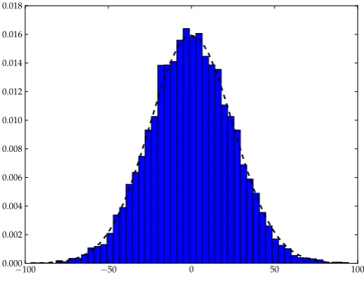
fixed velocity space grid is removed. In terms of the distribution function for a system of particles, the PIC method is a sampling of this distribution in phase space, illustrated in figure 2.1. PIC codes exhibit noise due to the fact the
−100 −50 0 50 100
[image:34.595.188.447.205.407.2]0.000 0.002 0.004 0.006 0.008 0.010 0.012 0.014 0.016 0.018
Figure 2.1: Histogram of the velocities of all particles in a cell between xand
x+ ∆x.
macro particles can contain a large number of particles, which is proportional
to 1/n2pic, where npic is the number of macro-particles per cell.
In the limit of infinite particles per cell, the PIC method can be show to be analogous to solving Vlasov’s equation. The choice then between a Vlasov code and a PIC code comes down to which one requires the least numerical effort for the same accuracy. Following the argument presented by Besse et al. [31] the ratio between the numerical effort(including both CPU and Memory requirement), between a Vlasov code and a PIC code will scale as:
Nvlas
Npart
,
same in both schemes, however this is not strictly true, and is dependent on the choice of interpolation scheme used in the PIC code.
The memory requirement for a Vlasov code is then the product of the number of points in each dimension in configuration and velocity space,
Nvlas=NxndxNvndv
wherendv andndx are the number of dimensions in velocity and configuration
space respectively. For a particle in cell code the numerical effort can be written as
Npart =n0∆xndxNxndx
wheren0 is the number of particles per cell. The graininess parameter due to
discrete particles in a PIC code can be defined as:
gpic=
1
n0∆xndx
Which is a measure of the numerical noise due to the finite number of particles used in a PIC simulation and is reduced by increasing the density of
macro-particles. For a PIC simulation,Npart can be written
Npart =g−pic1Nxndx
and the ratio is then.
Nvlas
Npart
=gpic(Nv)ndv
To capture kinetic effects such as wave-particle interactionsgpic is required to
be as small as possible to resolve the distribution function in the high velocity tails where such interactions occur. The discrete nature of a particle code means that the distribution function can be poorly resolved in regions of low mass. A Vlasov code however resolves all of phase space and does not have this problem. For 1D1P problems, Vlasov codes are always preferred over PIC codes. For 2 dimensional problems it depends on the levels of noise that can be tolerated in the PIC code for the particular problem. For 3 dimensions PIC codes are always preferred.
the tails of the velocity distribution. These energetic populations may only represent a tiny fraction of the total electron population and would therefore be poorly resolved using a PIC code.
2.2
The Vlasov-Maxwell System
The Vlasov equation for a single species is essentially the Boltzmann equation where the collision term is zero and where the forcing term is the Lorentz force. For a multi-species plasma, the particles interact through the effect they themselves have on the electric and magnetic fields which must be calculated self-consistently using Maxwell’s equations for moving charges. The Vlasov equation for a relativistic, multicomponent plasma is given by:
∂fj
∂t +
u
γ.∇xfj+
qj
mj
(E+ u
γ ×B).∇ufj = 0 (2.1)
Where the j subscript denoted the particle species. The fields must obey
Maxwell’s equations:
∇.E = ρ(x, t)
0
(2.2)
∇.B = 0 (2.3)
∇ ×E = ∂B
∂t (2.4)
∇ ×B =µ0J +0µ0
∂E
∂t (2.5)
Maxwell’s equations must be solved with the Vlasov equation in a self-consistent way. Thus, he number density of each species is defined by its distribution function
nj(x) =
Z
fj(x,u)du (2.6)
And the charge and current density:
ρ(x) =X
j qj
Z
fj(x, udu) (2.7)
J(x) =X j
qj Z
u
2.3
Numerical Schemes and the VALIS code
VALIS [32] is a code developed at Warwick by Tony Arber and Nathan Sir-combe that solves the relativistic Vlasov-Maxwell system in up to 2 spatial and 2 velocity dimensions; a 2D2P system. In this geometry the components
of the electric field, E = (Ex, Ey,0) and equations 2.4 and 2.5 become
∂Ex
∂t =−Jx+
∂Bz
∂y (2.9)
∂Ey
∂t =−Jy −
∂Bz
∂x (2.10)
∂Bz
∂t =−
∂Ex
∂y −
∂Ey
∂x (2.11)
with the electron density and current defined as
ne =
Z
fedu (2.12)
Jx,y =−
Z
ux,y
γ fedu (2.13)
There are no Bx, By components generated in this system so only Bz
needs to be calculated.
2.3.1
Simulation Grid
The 2D2P model of the distribution function is described on a 4D phase-space grid. Valis uses a staggered mesh similar to a Yee mesh [33] commonly used
in finite difference solvers. This is a fixed Eulerian grid running fromxmin to
xmax and ymin to ymax in the two spatial dimensions and −uxmax to uxmax in
ux and−uymax touymax inuy. The spatial and velocity grid cells are shown in
figure 2.2.
Figure 2.2: Left shows the spatial grid cell used in Valis. The distribution function is defined at the center with the fields defined at the cell boundaries.
Right shows the momentum grid cell. The advection co-ordinates ax,y are
defined at the cell boundaries and the distribution function, andhx,y are defined
in the center [32].
into account the relativistic factorγ. For the spatial advections define
hx(m, n) =
ux(m)
p
1 +u2
x(m) +u2y(n)
(2.14)
hy(m, n) =
uy(m)
p
1 +u2
x(m) +u2y(n)
(2.15)
and for the momentum space advections:
ax(m, n) =
ux(m)
q
1 +u2
x(m) + (
uy(n)+uy(n+1)
2 )2
(2.16)
ay(m, n) =
uy(m)
q
1 +u2
y(m) + (
ux(m)+ux(m+1)
2 )2
(2.17)
Non-Uniform Velocity Grid
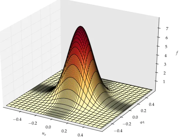
veloc-ity grid must resolve velocveloc-ity space up to these velocities at all times in the simulation. This is a major drawback of Vlasov codes. This problem can be somewhat diminished by concentrating grid points in areas where the distri-bution function has the most mass. This can also increase the accuracy of the numerical scheme at points where gradients in velocity space are the greatest. An illustration of a non-uniform velocity grid for a 2P distribution is shown in figure 2.3.
ux
−0.4
−0.2 0.0
0.2 0.4
uy
−0.4
−0.2 0.0
0.2 0.4
f
[image:39.595.188.493.277.512.2]1 2 3 4 5 6 7
Figure 2.3: Non-Uniform grid spacing to increase resolution aroundux =uy =
0
2.3.2
Updating the Distribution Function
∂f
∂t +v
∂f
∂x −E
∂f
∂v = 0 (2.18)
Rather than solving 2.18 as a whole at each timestep, split the update into two steps. First solve
∂f
∂t +v
∂f
∂x = 0 (2.19)
for half a timestep, then solve
∂f
∂t +E
∂f
∂v = 0 (2.20)
for a full time step then complete the second half of the spatial advections. The result is then an approximation to equation 2.18. Using the same method, the distrubution function updates of the electromagnetic, relativistic 2D2P system solved by VALIS become the following 1D advections:
∂fe
∂t +hx
∂fe
∂x = 0 (2.21)
∂fe
∂t +hy
∂fe
∂y = 0 (2.22)
∂fe
∂t + (Ex+ayBz)
∂fe
∂ux
= 0 (2.23)
∂fe
∂t + (Ey −axBz)
∂fe
∂uy
= 0 (2.24)
The advance of the distribution function fromt to t+ ∆t is then
1. xadvection: advance 2.21 from t tot+ ∆t/2
2. y advection: advance 2.22 from t tot+ ∆t/2
3. ux advection: advance 2.23 from t tot+ ∆t/2
4. uy advection: advance 2.24 from t to t+ ∆t
5. ux advection: advance 2.23 from t+ ∆t/2 to t+ ∆t
6. y advection: advance 2.22 from t+ ∆t/2 to t+ ∆t
7. xadvection: advance 2.21 from t+ ∆t/2 to t+ ∆t
The x-y ordering is reversed on alternate timesteps to avoid any directional
bias and the timestep size ∆t is determined by the CFL condition such that
∆t=M IN(∆x/vmax,∆v/|E|max).
the distribution function is a method to accurately solve the 1D advection equations.
Advection Methods
Accurate numerical solutions to the 1D advection equation,
∂a
∂t +u
∂a
∂x = 0 (2.25)
are are often required in many fields of computational fluid dynamics. There are a number of different methods to carry out these advections, examples include predictor-corrector type schemes such as MacCormack’s method [35], or interpolation schemes.
Interpolation Schemes The computational grid is shown in figure 2.4.
Where xj+1/2 is the boundary between thejth and j+ 1st and ∆x=xi+1/2−
xi−1/2.
Cell j Cell j+1
Cell j-1
j-1/2 j+1/2
x
a
Δx
Figure 2.4: Computational grid with the function a defined at the centre of
each cell
The value at the centre is the average of the solution between xj−1/2
and xj+1/2,
anj = 1
∆xj
Z xj+1/2
x
A piecewise interpolation method constructs a functionφacross each individual cell which satisfies the condition
anj = 1
∆xj
Z xj+1/2
xj−1/2
φ(x)dx
The solution at the centre of a cell at a timetn+1=tn+ ∆t, is then the value
of the interpolated function at φ(x−u∆t),
anj+1= 1
∆xj
Z xj+1/2
xj−1/2
φ(x−u∆t)dx
Since we are dealing with a probability distribution function, the
in-terpolated function φ must meet certain requirements to keep the solution
physical. The method must not introduce false extrema or accentuate
exist-ing extrema, doexist-ing so could allow f < 0 or f > fmax which are not physical
solutions for Vlasov’s equation. If f > fmax it would imply that particles
with a velocity and position have joined and as such are joined at all times forwards and backwards. This would violate the reversibility of Vlasov’s equa-tion in time, a property shared by any purely advective equaequa-tion. A negative probability is of course unphysical. VALIS uses the PPM [36] interpolation scheme to perform the advection updates. To illustrate the advantages of this method over others, first consider a simple linear interpolation scheme, the
Flux Balance Method.
Flux Balance Method The interpolation function is piecewise linear and
discontinuous at cell boundaries. The constructed linear function is illustrated in figure 2.5.
Setting y = x/∆x (so that yi = i), the method constructs a piecewise
interpolation function φ(y) using the gradient between the values of U either
side of the current cell:
Di = (Ui+1−Ui−1) (2.26)
φ(y) =Ui+Diy, y∈[i−1/2, i+ 1/2] (2.27)
Figure 2.5: Linear Piecewise Function fitting. The interpolation function is
centered atiand uses the gradient between the points i−1 and i+ 1. Here it
is shown to introduce a false maxima ati+ 1/2
of the ith and (i+ 1th) cell is computed,
φi+1/2=
Z i+1/2
i+1/2−λ
φ(y)dy (2.28)
Finally the value of U at the later time-step is computed using the difference
of the flux in and out of the cell.
Uin+1=Uin−(φi+1/2−φi−1/2) (2.29)
This method however is only second order accurate in space and is capable of introducing false maxima and minima into the distribution function as shown in figure 2.5.
Piecewise Parabolic Method From Gudonov’s theorem it’s known that
any linear method that does not accentuate existing maxima and minima can,
at best be first order accurate [37]. The method used in VALIS is thePiecewise
Parabolic Method(PPM). It is an improvement on the previous scheme as the piecewise linear function is replaced by a piecewise parabolic function. The reconstruction is a quadratic function in the form:
The reconstructed function ¯u preserves the average across each cell i if
1
∆xi
Z xi+1/2
xi−1/2
fr(x)dx= ¯uni
Expressions for the function at the left and right hand boundaries are then:
uL,i =fr,i(xi−1/2) = c0,i−
1
2∆xic1,i+
1
4∆x
2 ic2,i
uR,i=fr,i(xi+1/2) =c0,i+
1
2∆xic1,i+
1
4∆x
2 ic2,i
Solving for each coefficient gives
c0,i = ¯uni −
1
12∆x
2 ic2,i
c1,i =
uR,i−uL,i
∆xi
c2,i =
6
∆x2
i
uR,i+uL,i
2 −u¯
n i
1. Use a fourth order interpolation scheme to compute values of U at the
cell boundaries(i.e., Ui+1/2 for each i. These values must be limited to
ensure that a false maxima is not introduced, (i.e.,Ui+1/2∈[Ui, Ui+1]))
2. Generate φ(y) in each cell as a parabolic function passing through the
boundary values which has the correct mean, i.e.,Ri+1/2
i−1/2 φ(y)dy=Ui.
3. Limitφin each cell such that if Ui is a local extremum, set φ=Ui across
all the cell. If the interpolating function φ(y) achieves and extremum in
the cell, reset one of the boundary values (makingφ discontinuous there)
so that φ is monotone and so that dyφ = 0 at the edge opposite to the
resetting.
This method, through its use of cellwise limiters, does not introduce any false extrema into the distribution function. The interpolation scheme is third order
accurate away from extrema and 1st order at extrema, due to setting φ =Ui
2.3.3
Updating the Fields
The scheme to update the fields must be accurate, stable and scalable. Numer-ical schemes for solving Maxwell’s equations can potentially suffer cumulative error in the solution of Poisson’s equation or alter the dispersion relation. The scheme must avoid these and must do so without incurring significant compu-tational cost.
A Predictor Corrector scheme is used in VALIS. In this scheme, the
magnetic field is advanced from a time k−1/2 to k+ 1/2, then interpolating
back to findB at time k. The currents are integrated onto the spatial grid at
the cell faces. Here the integrated currents are denoted by ˜J and the number
of cells in (x, y, ux, uy) is given by (nx, ny, nux, nuy):
˜
Jxk(i, j) =−
nux X m=1 nuy X n=1
hx(m, n)fek(i, j, m, n)∆ux(m)∆uy(n) (2.30)
˜
Jyk(i, j) = −
nux X m=1 nuy X n=1
hy(m, n)fek(i, j, m, n)∆ux(m)∆uy(n) (2.31)
In the Yee mesh used in VALIS, the currents are required at the cell faces, so linear interpolation is applied:
Jxk(i, j) = 0.5( ˜Jxk(i, j) + ˜Jxk(i+ 1, j)) (2.32)
Jyk(i, j) = 0.5( ˜Jxk(i, j) + ˜Jxk(i, j+ 1)) (2.33)
The first order predictor forEx,yk+1/2 is then:
Exk+1/2(i, j) = Exk(i, j) + ∆t
2∆y(B
k
z(i, j)−B k
z(i, j−1))−
∆t
2 J
k
x(i, j) (2.34)
Eyk+1/2(i, j) = Eyk(i, j) + ∆t
2∆y(B
k
z(i, j)−B k
z(i−1, j))−
∆t
2 J
k
y(i, j) (2.35)
Now the distribution function can be advanced by a complete timestep
via the PPM method described earlier usingBkz+1/2 and Ex,yk+1/2
the previous timestep and the new timestep:
Jxk(i, j) = 0.5(Jxk(i, j) +Jxk+1(i, j)) (2.36)
Jyk(i, j) = 0.5(Jyk(i, j) +Jyk+1(i, j)) (2.37)
WhereJx,yk+1(i, j) is calculated using the updated distribution function at time
k+1. Now Ex,y can be advanced from k to k+1:
Exk+1(i, j) =Exk(i, j) + ∆t
∆y(B
k+1/2
z (i, j)−B k+1/2
z (i, j−1))−∆tJ k+1/2 x (i, j)
(2.38)
Eyk+1(i, j) =Eyk(i, j) + ∆t
∆x(B
k+1/2
z (i, j)−Bzk+1/2(i−1, j))−∆tJyk+1/2(i, j) (2.39) An illustration of the Valis algorithm is shown in figure 2.6.
For PIC(particle in cell) based codes, the charge density and current is often calculated by interpolating from the individual super-particles. While this scheme does satisfy charge conservation, it is known [38] however that the charge density and current does not satisfy the finite difference approximation of charge conservation as the system is advanced in time. As a result of this, these schemes do not satisfy Poisson’s equation as time is advanced, even if it is imposed at the start. The solution to this problem for PIC schemes is to calculate the charge that crosses the cell boundaries, rather than interpolat-ing from the particles [38]. This also all applies to direct Vlasov solvers. If the charge and current densities are calculated at grid points by integrating the distribution function and interpolating, there is no guarantee that charge conservation or Poisson’s equation is satisfied. If the current used in the field update is calculated using the flux through the edges of each computational cell, these fluxes are exactly those used to update the distribution function, so they must satisfy the finite difference version of the finite difference equation and therefore must satisfy Poisson’s equation to machine precision.
Fortunately thePPM method used in the 1D advections of the
distribu-tion calculates the flux of the distribudistribu-tion funcdistribu-tion through the edges of each
of the computational cells. This data can be recycled and used in thePredictor
Corrector approach.
the average current over the timestep. For each cell (i,j), Jx,yk+1/2 is defined as:
Jxk+1/2(i, j) =− 1
∆t
nux X
m=1 nuy X
n=1
hx(m, n)[∆tφkx+1(i, j, m, n)]∆ux(m)∆uy(n)
(2.40)
Jyk+1/2(i, j) =− 1
∆t
nux X
m=1 nuy X
n=1
hy(m, n)[∆tφky+1(i, j, m, n)]∆ux(m)∆uy(n)
(2.41)
whereφkx,y+1(i,j,m,n) is the flux through the positive direction cell boundary for
cell (i,j,m,n), as calculated in the PPM advection scheme during the advance of the distribution function from k to k+1. By performing a corrector step using the exact currents from the advection, VALIS ensures that Poisson’s equation is satisfied to machine precision, without any additional computational cost.
The field updates in Valis are fully explicit and require the time step to resolve the plasma period for electrostatic simulations and the minimum
of the plasma period and ∆x/c for electromagnetic simulations. This explicit
Figure 2.6: The Predictor Corrector approach used in Valis. This image is reproduced from Sircombe [32]
2.4
Normalisation
VALIS uses normalised units to avoid having to deal with numerical issues when dealing with extremely large and small numbers. The difference of var-ious quantities involved in a laser-plasma simulation can be many orders of magnitude in SI units, for example:
me = 9.1×10⁻³¹kg
c= 3×10⁸ms−1
By normalising, we choose a system of units where typical quantities are equal to 1. In Valis, masses are normalised to the electron mass, velocity to the speed of light, time to the plasma frequency and distance to the Debye length. Other units are then derived from these quantities. Table 2.1 shows all the normalised units used in Valis, where the units with marked with a tilde are normalised quantities and those without are in SI units.
However, for non-relativistic, electro-static simulations velocity is
nor-malised to the thermal velocity,v0=
q kBT0
tempera-Mass m=m0m˜ m0 =me
Velocity v =v0˜v v0=c
Distance x=x0x˜ x0= ωvpe0
Time t=t0˜t t0 = ω1
pe
Temperature T =T0T˜ T0= m0c
2
kB
Electric Field E =E0E˜ E0=
ωpev0me
e
Magnetic Field B =B0B˜ B0 =
ωpeme
e
Table 2.1: Normalisations used in Valis
ture is specified manually. The normalising density is also specified manually, but is only used in the collision module.
2.5
Parallelisation Using MPI
2.5.1
Domain Decomposition
VALIS is parallelised using a domain decomposition scheme and uses the MPI API [42] to communicate between each compute node. It is parallel in each dimension of the 4D phase space and options exist to restrict parallelism to any number of dimensions. Inter-process communication is achieved by adja-cent processes exchanging ghost cells at the beginning of each time-step. The
storage for the local chunk is nx+4 as each process receives the grid points
-2:0from their left neighbour’s nx-2:nx cells. Each process then updates its
chunk of the distribution function from 1 to nx using the PPM method. An
illustration of a 1D1P example, where the domain is parallel only in the x
direction is shown in figure 2.7.
Decomposition in velocity space is implemented generally in the same way. Boundary conditions however can make things a little less straightfor-ward and require non-nearest neighbour communication. These cases will be discussed in the next section.
2.5.2
Synchronisation and Non-Blocking Communication
BOUNDARY BOUNDARY
Process: 1 2 3 4
nx-1:nx sent to process 2
1:3 sent to process 1
Vx
0 nx
0 nx_global
Figure 2.7: Illustration of the domain decomposition used in VALIS. Each
process stores a chunk, nx of the total number of grid points in x, nx global.
The storage for the local chunk isnx+4as each process receives the grid points
-2:0 and nx+1:nx+3 from their left and right neighbours respectively at the beginning of each time step.
when one process calls a subroutine to receive data it does not have to wait for another process to call a subroutine to send data before it continues execution. By doing this, the processes need only synchronise once at the end of the boundary exchange routines.
2.5.3
File IO
The output is handled using the MPIIO API which allows each process to write to a file without having to gather all the data on a single process. The output is in unformatted boundary with a custom file structure. Each block of data is preceded by a header containing information about its size, shape and
name etc. Readers for the .valisare available for IDL, ViSiT and Python.
2.5.4
Boundary Conditions
Since VALIS solves Vlasov’s equation on a discrete grid using a computer with finite resources, the extent of the domain must also be finite.
Periodic Periodic boundary conditions are a way of simulating an infinitely
large domain on a finite size grid. Here thex min and x max are connected as
if they were adjacent in space. A particle element with a velocity vx moving
Reflecting Reflecting boundary conditions invert the distribution function
at the boundary so the value of f(vx) is copied into f(−vx) and vice versa.
For the fields the boundary value simply set equal to the adjacent cell. For
example,Ex(0) =Ex(1) and Ex(nx) =Ex(nx−1).
Laser A laser can be implemented at the boundary by simply driving
com-ponents of the electric field at a given frequency. This boundary is valid on the condition that the density of the plasma at the boundary is lower than the
critical density [43] , where ncrit[cm−3] = 1.121
1µm
λL
2
2.6
Numerical Tests
2.6.1
Landau Damping
Linear Landau damping of a Langmuir wave is a problem that is able to test a number of features of a Vlasov code. The electron distribution function is initialised with a density perturbation in configuration space. The advections
then lead to a perturbed velocity distribution function,f1, which varies asf1∼
eikvt. Hence there comes a time when the effective wavelength of this perturbed
velocity distribution is equal to twice the grid spacing. This filamentation needs to be dissipated in a physically consistent way, that does not introduce false
maxima, or allowf to become negative. The Piecewise Parabolic Method does
this by limiting the gradients inside each cell to ensure that iff is an extremum
at one of the cell boundaries, it never exceeds it inside. In this case it uses a first order approximation where the interpolation function inside the cell is a horizontal line which is the average of both boundaries, thus dissipating the filamentation and ensuring increasing entropy.
For this test the initial distribution function for the electrons is:
fe = (1 +αcos(kx)) exp(−ve2/2)/
√
2π
With the amplitude of the perturbation, α = 0.01, and k = 0.5 with
Lx = 4π. The velocity grid runs from (−vemax, vmaxe ) where vemax = 4.5. The
ions are stationary. Here the number of spatial grid points, Nx is fixed at 32
and the number of velocity grid points is varied asNv = 16,32,64 and 128. The
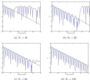
time in figure 2.8.
0 10 20 30 40 50
t(Plasma Periods)
−12 −10 −8 −6 −4 −2 0 E1
(a) Nv = 16
0 10 20 30 40 50
t(Plasma Periods)
−12 −10 −8 −6 −4 −2 0 E1
(b)Nv = 32
0 10 20 30 40 50
t(Plasma Periods)
−12 −10 −8 −6 −4 −2 0 E1
(c) Nv = 64
0 10 20 30 40 50
t(Plasma Periods)
−12 −10 −8 −6 −4 −2 0 E1
[image:52.595.136.509.162.492.2](d) Nv = 128
Figure 2.8: Linear Landau Damping of a Langmuir Wave
These initial conditions are identical to those in Arber and Vann [44],
and the damping rate obtained using the linear dispersion relation,γ = 0.153359.
A straight line is plotted through the peaks ofloge(E1), and its gradient yields
the damping rate obtained numerically. Ignoring the electric field, the solution to Vlasov’s equation is simply free streaming at each point in velocity space,
i.e. ∂f /∂t = v∂f /∂x. In this case each row in velocity space will be back
in its initial condition after a time, TR = 2π/(k∆v). For small initial E, the
solution will show signs of recurrence at times close toTR. An example of this
is evident in figure 2.8 where Nv is small, hence ∆v is large. In figure 2.8(a)
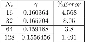
Nv γ %Error
16 0.160364 4.568
32 0.165704 8.05
64 0.159188 3.8
[image:53.595.246.394.107.182.2]128 0.1556456 1.491
Table 2.2: Percentage Error in the Damping Rate for Various Resolutions in Velocity Space
of the damping rate, the line is fitted only through the peaks wheret < TR/2,
which is different for each Nv. The percentage error in the damping rate for
2.7
Summary
Chapter 3
A Phenomenological
Approach to Collisions: the
Krook Model
3.1
Introduction
It’s clear that a reduced collision operator that is accurate, stable and fast would be desirable, given the already complex Vlasov system. The Bhatnagar-Gross-Krook(BGK) [18] collision operator simply assumes that collisions act to relax the system to an equilibrium distribution function at the collisional rate:
∂f
∂t
c
=−ν(v) (f−F) (3.1)
whereν is the velocity dependant collision frequency and F is the equilibrium
distribution. The equilibrium distribution is a Maxwellian with the density,
centre of mass velocity and temperature off. This collision term is added to the
right hand side of the Vlasov equation. After this point, the Vlasov equation with a collision operator shall be referred to as the Boltzmann equation.
A solution to the Boltzmann equation must be conservative, it must conserve particles, energy and momentum. For a homogenous plasma, it must
the production of entropy:
S=−k
Z
flogf dv
is always positive. This is true for the BGK operator since [21]
−k
Z
logf.(−ν(v)(f−F))dv=−k
Z
logf.(−ν(v)(f−F))dv
+k
Z
logF.(−ν(v)(f −F))dv
=k
Z
ν(v) log f
F(f−F)dv≥0
The equilibrium distribution distribution is the Maxwell-Boltzmann distribu-tion since,
ν(v)(f−F) = 0
when f =F. Furthermore the operator must maintain positive f. There are
no physical parameters to F that could cause f to become negative. Here we
use a velocity dependant collision frequency, which in the next section, will be shown to be implemented in a way that can conservers particles, energy and momentum.
![Figure 1.1: Fuel Capsule Prototype at the National Ignition Facility [8]](https://thumb-us.123doks.com/thumbv2/123dok_us/9559433.460542/14.595.248.393.108.227/figure-fuel-capsule-prototype-national-ignition-facility.webp)
![Figure 2.6: The Predictor Corrector approach used in Valis. This image isreproduced from Sircombe [32]](https://thumb-us.123doks.com/thumbv2/123dok_us/9559433.460542/48.595.165.470.116.345/figure-predictor-corrector-approach-valis-image-isreproduced-sircombe.webp)