Diffuse interface models of soluble surfactants in two phase fluid flows

(1)

University of Warwick institutional repository: http://go.warwick.ac.uk/wrap

A Thesis Submitted for the Degree of PhD at the University of Warwick

http://go.warwick.ac.uk/wrap/62686

This thesis is made available online and is protected by original copyright.

Please scroll down to view the document itself.

(2)

Diffuse Interface Models of Soluble Surfactants in

Two-Phase Fluid Flows

by

Kei Fong Lam

Thesis

Submitted to the University of Warwick for the degree of

Doctor of Philosophy

Mathematics Department

(3)

List of Tables

2.1 Possible functional forms for energy densities . . . 27

4.1 Convergence table for Model A, (α= 1) . . . 70

4.2 Convergence table for Model A, (α=ε), Henry isotherm . . . 73

4.3 Convergence table for Model A, (α=ε), Langmuir isotherm . . . 73

4.4 Convergence table for Model B, instantaneous adsorption . . . 75

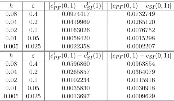
5.1 h, ε-convergence table for Neumann problem,ε= 4h . . . 132

5.2 h, ε-convergence table for Robin problem, ε= 4h . . . 132

5.3 h, ε-convergence table for Dirichlet problem, ε= 4h . . . 133

(7)

List of Figures

1.1 Emulsions and their stability . . . 1

1.2 Basis of diffuse interface models . . . 8

1.3 Typical potentials in phase field models . . . 8

4.1 1D Numerics, Model A, (α= 1),ε-convergence . . . 71

4.2 1D Numerics, Model A, (α=ε), ε-convergence . . . 72

4.3 1D Numerics, Model B,ε-convergence . . . 74

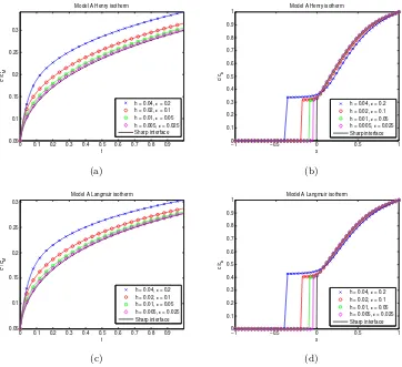
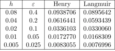
4.4 Droplet in shear flow, interface position for several isotherms . . . . 77

4.5 Droplet in shear flow, interface surfactant density and surface tension 77 4.6 Droplet in shear flow,α-convergence . . . 78

4.7 Marangoni effect on a surfactant laden droplet . . . 79

5.1 (Top) Double-obstacle regularisation δε. (Bottom) Finite element approximations of the bulk and surface solution ath= 0.05/√2 and ε= 2h . . . 135

(8)

Acknowledgments

First and foremost, I thank my supervisors Dr Bj¨orn Stinner and Professor Charles Elliott for their guidance and support over the years. They have introduced me to a rich field of mathematics and constantly encouraged me to play an active role in numerous conferences. I extend my thanks to Harald Garcke, Helmut Abels, Andreas Dedner, Vanessa Styles, Tom Ranner and Andrew Duncan for their valuable insights and remarks. Our discussions have greatly improved the quality of the work in this thesis. I also thank EPSRC and Charlie Elliott for the grant EP/H023364/1 and the creation of the MASDOC DTC programme. It came at a critical time when I was unsure about my future. Taking part in the programme reaffirm my desire to do research, and brought about tremendous amounts of personal development.

Next, I thank my housemates (Mike, Praveen, Chris and Simon) for making my time at 101 Canley Road one of the best experiences I had. Extra thanks go to my co-MASDOCers in the department for often putting up with my mischief and sometimes playing along. Their contributions to a relaxed and vibrant atmosphere make it so hard to leave.

Many thanks to the administration team for make this journey as smooth as possible. I appreciate the effort they put in behind the scenes to ensure there is minimal disruptions to our research time. I also thank Dave Wood for allowing me to gain valuable teaching experience.

(9)

Declarations

I declare that this thesis contains entirely my own research, conducted under the supervision of Bj¨orn Stinner and Charles Elliott, except where otherwise stated. It has not been submitted for a degree at any other university. It has not been submitted for award at any other institution or for any other qualification.

The material in Chapters 2, 3 and 4 are taken from a paper co-authored with Harald Garcke and Bj¨orn Stinner and published in Communications in Mathematical Science [Garcke et al., 2014]. The 2D simulations presented in Section 4.2.2 and the idea of Model C are due to Bj¨orn Stinner, while the reformulation of the surfactant equations, energy inequality for the phase field model, alternate asymptotic analysis for Model A and the asymptotics of Model B using the flux expansion are due to Harald Garcke.

(10)

Abstract

Surface active agents (surfactants) reduce the surface tension of fluid inter-faces and, via surface tension gradients, can lead to tangential forces resulting in the Marangoni effect. Biological systems take advantage of their impact on fluids with interfaces, but surfactants are also important for industrial applications such as processes of emulsification or mixing.

Surfactants can be soluble in at least one of the fluid phases and the ex-change of surfactants between the bulk phases and the fluid interfaces is governed by the process of adsorption and desorption. One can compute the interfacial sur-factant density from the bulk sursur-factant density by assuming that the interface is in equilibrium with the adjacent bulk phase and imposing a closure relation (known as adsorption isotherm) between the two quantities. The assumption (known as instantaneous adsorption) is valid when the process of adsorption to the interface is fast compared to the kinetics in the bulk phases. However, it is not valid in the context of ionic surfactant systems, or when the diffusion is not limited to a thin layer.

In this thesis, we derive two types of mathematical models for two-phase flow with a soluble surfactant that can account for both instantaneous and non-instantaneous adsorption. The first type is a sharp interface model, in which the interface is modelled by moving hypersurfaces. While the second type is a phase field model, in which the interface is a region of small, nonzero thickness where there is some microscopic mixing of the two fluids. Both types of models are shown to satisfy energy inequalities which guarantee thermodynamical consistency.

Via a formal asymptotic analysis, we show the phase field models are related to sharp interface models in the limit that the interfacial width tends to zero. Flexi-bility with respect to the choice of bulk and surface free energies allows us to realise various isotherms and relations of state between surface tension and surfactant. We present some numerical simulations to support the asymptotic analysis and display the effectiveness of the our approach.

(11)

Chapter 1

Introduction

1.1 Surfactants in emulsification

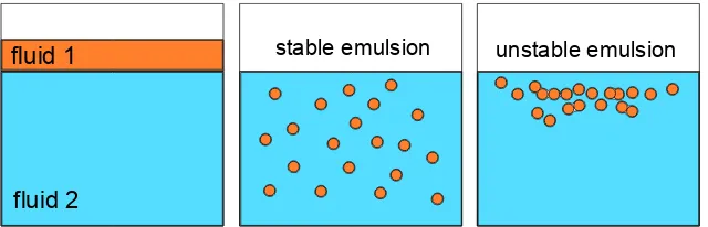
Emulsification is an important industrial process that involves mixing two or more fluids that normally are unmixable. More precisely, in the process of emulsification, it is desirable to have stable dispersions of one fluid in another (see Figure 1.1). Common examples of emulsions are milk, fire extinguishers and hand cream. The mixture is thermodynamically unstable and will progressively revert back to their unmixed states over time. Surface active agents (or surfactants) are often added to increase the stability of the mixture and hence there is great interest, especially in industrial applications, to understand the influence of surfactants on the dynamics of multi-fluid systems.

fluid 1

fluid 2

[image:11.595.162.482.488.591.2]

unstable emulsion stable emulsion

Figure 1.1: Two immiscible fluids that are not yet emulsified. If the surface tension between the fluids are reduced, one might see that fluid 1 enters a dispersed phase and is dispersed into fluid 2. The emulsion is termed stable if one fluid is fully dispersed in the other. Otherwise, an unstable emulsion will progressively separate. Surfactants are often used to reduce the surface tension between the fluids, and thus stabilising the emulsions.

(12)

tension between the two fluids exist due to the immisicibility of the fluids and emulsification takes place when the tension between the two fluids is low enough. By adhering to the interfaces and creating a buffer zone, surfactants reduce the surface tension of the interfaces, which permits stability of small droplets of one fluid suspended in a bulk of the other fluid.

Moreover, the local differences in surface tension can cause surfactants to diffuse along the interface, a phenomenon known as the Marangoni effect. This in turn changes the shape of the interface and leads to more diffusion of the surfactants. This complex coupling between surfactants and the fluids is at the heart of many industrial processes involved in emulsification.

Surfactants can be broadly classified into soluble and insoluble surfactants. While soluble surfactants can exist in the bulk fluid phases and on the interface, surfactants that are insoluble will only exist within the interface, and so when intro-duced to a multi-fluid system, they will migrate towards the interface by the process of adsorption. Much previous work have been done to understand the process of adsorption and to postulate a model for surfactant dynamics.

One of the simplest models for adsorption dynamics is the model of Ward and Tordai [1946]. Consider a semi-infinite region Ω := (0,∞) with interface Γ = {0}. Let the bulk surfactant concentration in Ω be given byc and the interfacial surfac-tant concentration be given bycΓ_{. We also define the sub-layer or the sub-surface to} be the bulk region immediately next to the interface. On the assumption that equi-librium between the sub-layer and the interface is established instantaneously (this is known as diffusion controlled adsorption or instantaneous adsorption [Diamant and Andelman, 1996]), the model of Ward and Tordai [1946] reads as:

∂c ∂t =D

∂2c

∂x2 forx >0, t >0,

∂cΓ ∂t =D

∂c

∂x atx= 0, t >0,

with initial and boundary conditions lim

x→∞c(x, t) =cb fort >0, c(x,0) =cb, c

Γ_{(0) = 0}_.

In their work, Ward and Tordai derived an expression forcΓ:

cΓ(t) = 2

r

D π cb

√

t−

Z √

t

0

c(0, t−τ)d√τ

!

(13)

where c(0, t) is the concentration in the sub-layer. Since the sub-layer and the interface are in equilibrium, we can impose a relation betweenc(0, t) andcΓ(t):

c(0, t) =g(cΓ(t)),

for some function g. This functional relation is often termed adsorption isotherm, which relates the concentration in the sub-layer with the concentration on the in-terface. More importantly, the Ward–Tordai equation becomes:

cΓ(t) = 2

r

D π cb

√

t−

Z √

t

0

g(cΓ(t−τ))d√τ

!

,

and a Newton method can be employed to solve forcΓ₍_t_{) (see [Li et al., 2010]).} Several hypotheses have been proposed regarding the form for the adsorption isotherm, leading to the development of forms for g. Table 2.1 displays six of the isotherms used in the literature, those of Henry, Langmuir, Volmer, van der Waals, Freundlich, and Frumkin (see also [Eastoe and Dalton, 2000; Kralchevsky et al., 1999, 2008]), along with the functional forms for the interfacial free energy density

γ(cΓ_{), the bulk free energy density} _G₍_c_{) and the surface tension}_σ₍_cΓ_).

We remark that the central assumption to the Ward–Tordai equation is that the sub-layer and the interface are in thermodynamical equilibrium at all times, i.e. the process of adsorption is fast compared to the kinetics in the bulk regions. This corresponds to the case of diffusion-limited adsorption studied in Diamant and Andelman [1996]. However, instantaneous adsorption is not valid in the context of ionic surfactant systems [Diamant and Andelman, 1996] or when the diffusion is not limited to a thin layer [Coutelieris, 2002; Coutelieris et al., 2003, 2005]. In these situations, we will not have a closure relation for c(0, t) and cΓ(t). Therefore, we would like to develop models that are able to account for both instantaneous and non-instantaneous adsorption.

1.2 Sharp interface models

(14)

Let Ω denote an open bounded domain inRncontaining two fluids of different

mass densities. We denote by Ω(1)(t), Ω(2)(t) the domains of the fluids which are separated by an interface Γ(t). The sharp interface model is given as:

∇ ·v= 0,in Ω(i)(t), (1.2.1)

∂t(ρ(i)v) +∇ ·(ρ(i)v⊗v) =∇ ·

−pI+ 2η(i)D(v),in Ω(i)(t), (1.2.2)

∂_t•c(i)=∇ ·(M_c(i)∇G0_i(c(i))),in Ω(i)(t), (1.2.3) [v]2₁= 0, v·ν =uΓ,on Γ(t), (1.2.4) [pI −2η(i)D(v)]2₁ν =σ(cΓ)κν +∇_Γσ(cΓ),on Γ(t), (1.2.5)

∂_t•cΓ+cΓ∇Γ·v− ∇Γ·(MΓ∇Γγ0(cΓ)) = [Mc(i)∇G

0

i(c(i))]21ν,on Γ(t), (1.2.6)

α(i)(−1)iM_c(i)∇G0_i(c(i))·ν =−(γ0(cΓ)−G0_i(c(i))),on Γ(t). (1.2.7) Herev denotes the fluid velocity, ρ(i) is the constant mass density for fluidi,η(i) is the viscosity of fluidi,D(v) = 1₂(∇v+ (∇v)⊥) is the rate of deformation tensor,pis the pressure,I is the identity tensor,∂_t•(·) =∂t(·)+v·∇(·) is the material derivative,

c(i) is the bulk density of surfactant in fluidi,Mc(i) is the mobility of surfactants in fluidi, Gi(c(i)) is the bulk free energy density associated to the bulk surfactant in fluidi. On the interface, [·]2

1 denotes the jump of the quantity in brackets across Γ from Ω(1) to Ω(2),uΓ is the normal velocity,ν is the unit normal on Γ pointing into Ω(2), cΓ is the interfacial surfactant density, σ(cΓ) is the density dependent surface tension, κ is the mean curvature of Γ, ∇_Γ is the surface gradient operator, ∇_Γ· is the surface divergence, MΓ is the mobility of the interfacial surfactants, γ(cΓ) is the free energy density associated to the interfacial surfactant, and α(i) ≥ 0 is a kinetic factor that relates to the speed of adsorption. The above model satisfies the second law of thermodynamics in an isothermal situation in the form of an energy dissipation inequality.

(15)

In this model, the surface tension σ : R+ → R+, R+ := [0,∞), is a (usu-ally decreasing) function of the surfactant density cΓ. The phenomenon known as Marangoni effect, where tangential stress at the phase boundary leads to flows along the interface, is incorporated into the model via the surface gradient ofσ in the momentum jump free boundary condition (1.2.5).

We remark that if the setting is non-isothermal, the Marangoni effect can be caused by temperature gradients in the absence of surfactants. In this case, we will have one temperature fieldθ(i),i= 1,2,for each of the phases and they satisfy

∂tθ(i)+v· ∇θ(i)=κ(i)∆θ(i),in Ω(i)(t), [θ(i)]2₁ = 0, [κ(i)∇θ(i)]2₁ν = 0,on Γ(t),

where κ(i) is the thermal conductivity of fluid i. The surface tension σ is now a function (typically linear and decreasing) of the interface temperatureθ, defined as the averageθ= 1₂(θ(1)+θ(2))|_Γ(_t₎. The model of Rayleigh–Marangoni–B´enard con-vection in two-phase flow consists of the above equations involving the temperature fields, (1.2.1),(1.2.2),(1.2.4), and (1.2.5) with σ(θ) instead of σ(cΓ).

The model studied in Bothe, Pr¨uss, and Simonett [2005]; Bothe and Pr¨uss [2010] bears the most resemblance to the above model (1.2.1)−(1.2.7), where the setting of these papers is the diffusion-limited regime with a surfactant which is soluble in one phase only and (1.2.7) is replaced by the relation

γ0(cΓ) =G0(c) ⇐⇒ cΓ=g(c) := (γ0)−1(G0(c)), (1.2.8) in whichgplays the role of the equilibrium isotherm andGis the bulk free energy of the phase in which the surfactant is soluble. Our approach is based on a free energy formulation, originated from Diamant and Andelman [1996]; Diamant et al. [2001], where we gain access to equilibrium isotherms by setting α(i) = 0 and choosing suitable functions forγ and Gi. Furthermore, for positive values ofα(i) we are able to include the dynamics of non-equilibrium adsorption.

(16)

the most general existence result is the global in time existence of measure-valued varifold solutions of Abels [2007]. We also mention the results of Tanaka [1993]; Giga and Takahasi [1994]; Nouri and Poupaud [1995]; Denisova [2000]; Pr¨uss and Simon-ett [2010]; Xu and Zhang [2010]. For the two-phase Rayleigh–Marangoni–B´enard convection model, local in time existence has been proved in Tanaka [1995].

To the author’s best knowledge, the only existence result regarding classical models of soluble surfactants in two-phase flow is that of Bothe, Pr¨uss, and Simonett [2005], where short time existence of classical solutions to a one-sided version of (1.2.1)−(1.2.6),(1.2.8) for special configurations is shown. A subsequent analysis of the stability of equilibria can be found in Bothe and Pr¨uss [2010].

1.3 Phase field models

The governing equations (1.2.1)−(1.2.7) form a free boundary problem. The phase boundary Γ(t) is unknown a priori and hence must be computed as part of the solu-tion. Much work have been dedicated to explicitly tracking and capturing the inter-face using various numerical methods. Popular methods include level set methods [Xu et al., 2006; Gross and Reusken, 2011; Xu et al., 2014], front-tracking methods [Muradoglu and Tryggvason, 2008; Lai et al., 2008; Khatri and Tornberg, 2011], volume-of-fluid methods [James and Lowengrub, 2004; Alke and Bothe, 2009; Re-nardy et al., 2002] and arbitrary Lagrangian–Eulerian methods [Yon and Pozrikidis, 1998; Yang and James, 2009; Ganesan and Tobiska, 2009; Barrett et al., 2013].

Despite significant advances in the modelling and computation of two-phase flows, the sharp interface description breaks down when topological changes of the interface occur. Phenomena such as breakup of fluid droplets, reconnection of fluid interfaces, pinching, coalescence, cusp formation, and tip-streaming driven by Marangoni forces [Fernandez and Homsy, 2004; Krechetnikov and Homsy, 2004a,b] involve changes in the topology of the interface. At such an event, the fluid interface cannot be represented by a hypersurface and so the sharp interface equations are no longer valid. Numerically, complications also arise when the shape of the interface becomes complicated or exhibits self-intersections.

(17)

how to perform an interfacial reconnection [Unverdi and Tryggvason, 1992]. On the other hand, in a front-capturing method, the interface is embedded as a level set of a function defined throughout the computational domain. This formulation allows the numerical method to transition through a topological singularity without any additional intervention, but re-initialisation of the level set might be necessary for mass conservation or to maintain the signed distance property (see [Chang et al., 1996; Sussman et al., 1994]).

These difficulties have led to the development of diffuse interface (or phase field) models to provide an alternative description of fluid/fluid interfaces. At the core of these models, it is assumed that there is some microscale mixing of the macroscopically immiscible fluids and the sharp interface is replaced by an interfacial layer of finite width. Within this region the two fluids are mixed and the model has to account for certain mixing energies. An order parameter is introduced to distinguish between the fluids within the interfacial layer, where it takes distinct constant values in each of the bulk regions and varies smoothly across the narrow interfacial layer (see Figure 1.2). The original sharp interface can then be represented as the zero level set of the order parameter, which draws on ideas of the front-capturing method, thus allowing different level sets to exhibit different topologies. We mention the work of Lowengrub et al. [1999]; Lowengrub and Truskinovsky [1998] on the investigation of phase field models near topological transitions in the context of two-phase flows. We remark that, in contrast to the front-capturing method where the inter-face is represented as a level set of an artificial function, the order parameter in the phase field model can have physical meaning. For example, one can choose the order parameter to be the difference in volume fraction, the difference in mass concentra-tion or the density difference (see [Abels et al., 2011; Lowengrub and Truskinovsky, 1998]).

1.3.1 Choice of potentials

At the centre of the phase field models lies the Ginzburg–Landau energy density: E_GL(ϕ,∇ϕ) := ε

2|∇ϕ| 2₊1

εW(ϕ), (1.3.1)

(18)

[image:18.595.161.482.109.215.2]

Figure 1.2: The order parameter ϕ contains information about the location of the phases. If Ω(1) is the region where ϕ = −1 and Ω(2) _{is the region where} _ϕ ₌ +1, then in the sharp interface model, ϕ jumps across the interface. The phase field methodology replaces the original hypersurface Γ with an interfacial layer of thicknessεand allowsϕ to transition smoothly from one phase to the other.

for a potential of double-well type or

W(ϕ) = 1 2(1−ϕ

2_{) +}_I

[−1,1](ϕ), I[−1,1](ϕ) =







0, if |ϕ| ≤1,

∞, else,

for a potential of double-obstacle type (see Figure 1.3). The potential termW(ϕ) prefers the order parameter ϕ in its minima at ±1 and the gradient term |∇ϕ|2 penalises large jumps in gradient. This leads to the development of bulk regions whereϕis close to ±1 which are separated by a narrow interfacial layer.

−2 −1.5 −1 −0.5 0 0.5 1 1.5 2

0 0.1 0.2 0.3 0.4 0.5 0.6 0.7 0.8 0.9 1

Order parameter φ

Potentials W(

φ

)

Double−Well Double−Obstacle

Figure 1.3: The double well and double obstacle potentials. Notice that the double obstacle potential penalises heavily ifϕ /∈[−1,1].

[image:18.595.222.420.467.625.2]

(19)

double-well potential is that the order parameterϕmay not strictly lie in the interval [−1,1]. For order parameters that have physical meaning, such as the difference in volume fraction between two fluids, the physical interpretation ofϕ <−1 orϕ >1 is unclear. On the other hand, the penalty term I[−1,1](ϕ) of the double-obstacle potential confines ϕ to lie in the interval [−1,1], and so there is no ambiguity in identifying

ϕ with a physical parameter. A drawback of using a double-obstacle potential is that the resulting model equations are replaced by variational inequalities, and subsequent analysis of the models are more complicated than those with a double-well potential. We refer to Chen and Elliott [1994] for a discussion involving the two choice of potentials.

1.3.2 Phase field models for two-phase flow

The review Anderson et al. [1998] provides an overview on diffuse interface methods in the context of fluid flows. In Gurtin, Polignone, and Vi˜nals [1996]; Hohenberg and Halperin [1977] it was already proposed to combine a Cahn-Hilliard equation for distinguishing the two phases with a Navier-Stokes system. An additional term was included in the momentum equation to model the surface contributions to forces. In the case of different densities, Lowengrub and Truskinovsky [1998] derived quasi-incompressible models, where the fluid velocity is not divergence free. On the other hand, Ding, Spelt, and Shu [2007] has derived a diffuse interface model for two-phase flow with different densities and with solenoidal fluid velocities. But it is not known whether this model is thermodynamically consistent. Most recently, a phase field model for non-matched densities and divergence-free velocity that satisfies local and global energy inequalities has been derived by Abels, Garcke, and Gr¨un [2011].

(20)

1.3.3 Phase field models for surfactants in two-phase flow

Generalising the model of Abels, Garcke, and Gr¨un [2011], the second contribution of this thesis is the derivation of three diffuse interface models for soluble surfactants in two-phase flow. This is done in Chapter 3. For the case of non-instantaneous adsorption (α(i)>0), we will derive the following model (denoted Model A):

∇ ·v = 0, (1.3.2)

∂t(ρv) +∇ ·(ρv⊗v) =∇ ·

−pI + 2η(ϕ)D(v) +v⊗ ρ(2)−₂ρ(1)m(ϕ)∇µ (1.3.3) +∇ · σ(cΓ)(δ(ϕ,∇ϕ)I − Wε∇ϕ⊗ ∇ϕ),

∂•_tϕ=∇ ·(m(ϕ)∇µ), (1.3.4)

µ=−∇ ·(Wεσ(cΓ)∇ϕ) +W

ε σ(c

Γ₎_W0

(ϕ) (1.3.5) + X

i=1,2

ξ_i0(ϕ)(Gi(c(i))−G0i(c(i))c(i)),

∂_t•(ξi(ϕ)c(i)) =∇ ·(M_c(i)(c(i))ξi(ϕ)∇G0i(c(i))) (1.3.6) + 1

α(i)δ(ϕ,∇ϕ)(γ

0₍_cΓ₎₋_G0

i(c(i))), i= 1,2,

∂_t•(δ(ϕ,∇ϕ)cΓ) =∇ · MΓ(cΓ)δ(ϕ,∇ϕ)∇γ0(cΓ)

(1.3.7) −δ(ϕ,∇ϕ) X

i=1,2 1

α(i)(γ

0₍_cΓ₎₋_G0

i(c(i))).

Hereεis a length scale associated with the interfacial width,ϕis the order parameter that distinguishes the two bulk phases. In factϕtakes values close to±1 in the two phases and rapidly changes from−1 to 1 in an interfacial layer. The functionsξi(ϕ) andδ(ϕ,∇ϕ) act as regularisations to the Dirac measures of Ω(i)_{and Γ, respectively,} while W is a constant related to δ(ϕ,∇ϕ). Equations (1.3.2) and (1.3.3) are the incompressibility condition and the phase field momentum equations, respectively. Equation (1.3.4) together with (1.3.5) governs how the order parameter evolves and equations (1.3.6) and (1.3.7) are the bulk and interfacial surfactant equations, respectively.

(21)

bulk and interface surfactant equations (1.3.6), (1.3.7) with

∂_t•(ξ1c(1)) =∇ ·(Mc(1)(c(1))ξ1∇G01(c(1))) + 1

α(1)δ(G

0

2(c(2))−G01(c(1))), (1.3.8)

∂_t•(ξ2c(2)+δg(c(2))) =∇ ·((Mc(2)ξ2+MΓ(g(c(2))))δ∇G02(c(2))) (1.3.9) − 1

α(1)δ(G

0

2(c(2))−G01(c(1))), whereg(c(2)) is the adsorption relation as in (1.2.8).

The case where there is instantaneous adsorption in both bulk phases is covered by Model C, which consists of (1.3.2)−(1.3.5) and

∂•_t(ξ1c(1)(q) +ξ2c(2)(q) +δcΓ(q))−

X

i=1,2

∇ ·(Mi(c(i)(q))ξi∇q) (1.3.10)

− ∇ ·(MΓ(cΓ(q))δ∇q) = 0.

Here, q denotes a chemical potential where, as will be discussed in Chapter 3, we can express the surfactant densities as functions ofq.

The Model A is related to the approach in Teigen et al. [2009]. We modify the approach of Teigen et al. [2009] in such a way that an energy inequality is valid and such that we recover the isotherm relations for adsorption phenomena in the limit of instantaneous adsorption. We deepen the asymptotic analysis in that it works with the original equation for the surface quantity and does not require the assumption of extending the surface quantity continuously in the normal direction. We remark that Model B is more intuitive at considering instantaneous ad-sorption, since the relation (1.2.8) can be seen directly in surfactant equations. As we can expresscΓ _{as a function of} _c(2)_{, we add the equations for} _c(2) _and _g₍_c(2)_{) to} obtain (1.3.9). If we also consider instantaneous adsorption in Ω(1), then this would lead to the relation

(22)

1.3.4 Phase field models with two order parameters

Phase field models of surfactant adsorption that utilise the free energy approach of Diamant and Andelman [1996]; Diamant, Ariel, and Andelman [2001] can be traced back to the models of Theissen and Gompper [1999]; Teramoto and Yonezawa [2001]; van der Sman and van der Graaf [2006]. In contrast with Models A, B and C presented above, these phase field models employ two order parameters, Ψ and Φ, which describe the difference in the local densities of the fluids and the local concentration of surfactants, respectively. An energy functionalF(Ψ,Φ,∇Ψ,∇Φ) of Ginzburg–Landau type is then prescribed and the order parameters satisfy evolution equations of Cahn–Hilliard type with respect to the energy functionalF:

∂tΨ =MΨ∆µΨ, ∂tΦ =MΦ∆µΦ,

where µΨ := δF_δ_Ψ and µΦ := δF_δ_Φ are the first variations of F with respect to Ψ and Φ, respectively and MΨ, MΦ > 0 represent the (constant) mobilities of Ψ and Φ, respectively.

Hydrodynamics can be introduced to the model by coupling the Cahn– Hilliard type equations for Ψ and Φ with the Navier–Stokes equations, leading to the model of van der Sman and van der Graaf [2006] (see also Appendix A of [Engbolm et al., 2013]):

∇ ·v= 0,

ρ(∂tv+ (v· ∇)v) =−∇p+∇ ·(2ηD(v))−Φ∇µΦ−Ψ∇µΨ,

∂tΨ +v· ∇Ψ =∇ ·(MΨ∇µΨ),

∂tΦ +v· ∇Φ =∇ ·(MΦ∇µΦ).

The form ofµΦ andµΨwill depend on the form ofF(Ψ,∇Ψ,Φ,∇Φ). For a detailed numerical comparison of phase field models of this type, we refer the reader to [Li and Kim, 2012].

We observe that parameters such as the surface tension σ and the kinetic factor measuring local thermodynamic equilibrium α(i) do not appear explicitly in the twin order parameter type phase field models. In the derivation of the model equations, a desirable adsorption isotherm is first selected and the energy functional

(23)

so one can identify the chemical potential for the surfactants in the two bulk phases and on the interface. Local thermodynamic equilibrium is achieved by equating the chemical potentialsµΦ(Ψ = +1) =µΦ(Ψ =−1) =µΦ(Ψ = 0) and rearranging gives the adsorption isotherm (see [Liu and Zhang, 2010]).

Among the aforementioned models with hydrodynamics, the model of van der Sman and van der Graaf [2006] can only achieve the Langmuir isotherm, while the model of Liu and Zhang [2010] can achieve both the Langmuir and the Frumkin isotherms. With regards to this, we remark that our phase field models are more flex-ible that these twin order parameters type phase field models at recovering isotherms in thermodynamic equilibrium, since our surfactant equations do not have to be re-derived in order to facilitate changing isotherm relations.

1.4 Sharp interface limits of the phase field models

In the phase field models, the width of the interfacial layer is characterised by the length scale over which the order parameter varies from its values at the bulk regions. A natural question is whether the phase field model can be related to the sharp interface model in the asymptotic limit in which this width is small compared to the length scales associated to the bulk regions. If so, one can also view the phase field methodology purely as a tool for approximating the sharp interface equations. If the objective is to ensure that, in the limit of vanishing interfacial thickness, certain sharp interface models are recovered then there is a lot of freedom in constructing phase field models to meet one’s needs (see e.g. [Li et al., 2009]).

The results on the asymptotic limits of phase field models are broadly divided into two categories. One is based on formally matched asymptotic calculations, while the other consists of mathematically rigorous convergence results.

1.4.1 Formal asymptotics analysis

The procedure of formal asymptotic analysis is based on the assumption that there exist a family of solutions, sufficiently smooth and indexed by ε, to the diffuse interface models. For small ε, we assume that the domain Ω can at each time t

(24)

it is not analysed further and it is not known whether the asymptotic expansions really exist and converge. Details of the method can be found in Caginalp [1989]; Fife and Penrose [1995]; Garcke and Stinner [2006]; Abels, Garcke, and Gr¨un [2011] for the phase field models with the smooth double-well potential and in Blowey and Elliott [1993]; Cahn, Elliott, and Novick-Cohen [1996]; Bhate, Bower, and Kumar [2002] for phase field models with the double-obstacle potential.

The third contribution of this thesis is a formal asymptotic analysis of Models A, B and C with both the double-well and double-obstacle potentials. In Chapter 4, we highlight the differences in the analysis and show that Model A converges formally to the sharp interface model (1.2.1) - (1.2.7), while Models B and C converge formally to the case of one-sided and two-sided instantaneous adsorption, respectively. For Model A, by choosing α(i) to scale with ε, we formally recover the sharp interface model with two-sided instantaneous adsorption. The analysis of this case is slightly non standard and the details are presented in Section 4.1.4.

We remark that it is unknown if the twin order parameter type phase field models such as the model of van der Sman and van der Graaf [2006] can be related to any sharp interface model in the limit of vanishing interfacial thickness.

1.4.2 Rigorous convergence results

The techniques for showing rigorous convergence of phase field models are divided into two main categories. The first method is to rigorously justify the formal asymp-totic analysis, while the second is to show that weak solutions to the phase field models converge weakly to generalised solutions to the sharp interface equations.

Rigorous asymptotic analysis

The method of rigorous asymptotic analysis is based on constructing an approxi-mating solution that almost satisfy the phase field equations (i.e. with an additional error term) and converges strongly to classical solutions to the sharp interface equa-tions. This implies that classical solutions to the sharp interface model are required to apply this technique.

(25)

there exists a region where both expansions are valid and hence should match up). This allows us to construct an expansion of arbitrary order inεand it can be shown that this expansion satisfy the phase field equations with an additional “error” term. Via some spectral estimates from Chen [1994], one can show that, as the order of the expansion increases, the error term can be made arbitrary small and hence the constructed expansion is arbitrary close to the solution to the phase field equations. Moreover, the leading order term in the expansion is constructed from the classical solution to the sharp interface equations. Hence, asε→0, the solutions to the phase field equations converge strongly to the classical solution to the sharp interface equations.

We remark that this method has been successfully applied to the Allen–Cahn equation [De Mottoni and Schatzman, 1995], the Cahn–Hilliard equation [Alikakos et al., 1994; Carlen et al., 2005], and for a general phase field model [Caginalp and Chen, 1998].

Energy methods and weak convergence

One may also take advantage of the natural a priori estimates (or energy estimates) that some of the phase field models possess. These estimates provide uniform bounds on certain quantities and allow us to deduce compactness results. For instance, one observes that the Allen–Cahn equation

ε∂tϕAC =ε∆ϕAC− 1

εW

0

(ϕAC), in Ω, ∇ϕAC·ν∂Ω= 0, on∂Ω, and the Cahn–Hilliard equation

ε∂tϕCH = ∆µ, µ=−ε∆ϕCH+ 1

εW

0₍_ϕ

CH),in Ω, ∇ϕCH ·ν∂Ω=∇µ·ν∂Ω= 0,on∂Ω, possess the following natural a priori estimate:

Z

Ω

E_GL(ϕAC,∇ϕAC)(t) +

Z t

0

Z

Ω

ε|∂tϕAC|2 =

Z

Ω

E_GL(ϕAC,∇ϕAC)(0),

Z

Ω

EGL(ϕCH,∇ϕCH)(t) +

Z t

0

Z

Ω

|∇µ|2 =

Z

Ω

EGL(ϕCH,∇ϕCH)(0).

(26)

weakly in appropriate function spaces. The weak limit is then shown to be the weak/generalised solution of the sharp interface model.

In the radial symmetric case, rigorous convergence based on energy methods have been shown in Stoth [1996] for the Cahn–Hilliard equation and in Bronsard and Kohn [1991] for the Allen–Cahn equation. In Blowey and Elliott [1994], weak solutions to a phase field model with a double–obstacle potential are shown to converge to the weak solution to the classical Stefan problem.

In general, weak solutions to classical free boundary problems may develop singularities in finite time and it becomes unclear how to define classical solutions to the sharp interface problems. Brakke [1978] made a first attempt to define gener-alised solutions to motion by mean curvature, where the existence of a weak solution to the mean curvature flow is shown in the class of codimension-one varifolds. Subse-quently, using energy bounds and techniques from geometric measure theory, Ilma-nen [1993] showed that the weak solutions to the Allen–Cahn equation converges to mean curvature flow in the sense of Brakke [1978]. This technique has been success-fully applied to the Cahn–Hilliard equation and its variants in Chen [1996]; R¨oger and Tonegawa [2008]; Garcke and Kwak [2006], and to a general phase field model in Soner [1995]. For two-phase flow, the convergence of weak solutions of the Abels, Garcke, and Gr¨un [2011] model to varifold solutions of a Navier–Stokes/Mullin– Sekerka system has been shown in Abels and Lengeler [2013].

The energy method has also been applied in the setting of numerical approx-imation of phase field models. In a series of papers [Feng and Probl, 2003, 2004, 2005], Feng and Prohl have proposed various finite element approximations to phase field models that utilise spectral estimates of the Allen–Cahn and Cahn–Hilliard op-erators derived in Chen [1994] to establish useful a priori bounds that grow only in low polynomial order of ε−1_{, under reasonable constraints on the underlying finite} element mesh. They show that the fully discrete solutions converge to the solutions of the phase field models as the spatial and temporal mesh sizes tend to zero and, as a non-trivial byproduct, the fully discrete solution converges to classical solutions of the sharp interface models asεconverges to zero.

(27)

the fourth contribution of this thesis is the analysis and convergence of a diffuse interface approximation to an elliptic coupled bulk-surface PDE system with the energy method. We will show, in Chapter 5, that the weak solutions (uε_{, v}ε_{) to}

−∇ ·(ξεAE∇uε) +ξεaEuε=ξεfE+δεK(vε−uε), in Ω, −∇ ·(δεBE∇vε) +δεbEvε=δεβgE−δεK(vε−uε), in Ω.

(1.4.1)

converge to the weak solution (u, v) to

−∇ ·(A∇u) +au=f,in Ω(1),

−∇_Γ·(B∇_Γv) +bv+A∇u·ν =βg,on Γ =∂Ω(1),

A∇u·ν=K(v−u),on Γ.

(1.4.2)

asε→0, where Ω(1) is a domain contained in Ω such that Γ∩∂Ω =∅,AE_,_aE_,_fE_, BE_,_bE_,_gE _{are extensions of} _A,_a_,_f_,_B,_b_,_g _{to Ω, and}_ξ

ε and δε are similar to the corresponding functions in Models A, B and C.

Sub- and super-solutions

For completeness, we mention the method of sub- and super-solutions, which will not be used in this thesis. For phase field models consisting of second order differential equations, the comparison principle provides another technique to show rigorous convergence to solutions of the sharp interface equations. The idea is to construct sub- and super-solutions to the phase field model using the classical solutions of the sharp interface equations. The comparison principle implies that the solution to the phase field model is bounded above and below by the super- and sub-solution, respectively, provided their initial conditions are related in a similar way. One can show that the Hausdorff distance between the zero-level set of the order parameter and the sharp interface hypersurface scales withε.

This method has been applied predominantly to the Allen–Cahn equation and its variants, we refer to Evans et al. [1992]; Alfaro et al. [2008]; Chen [1992a,b]; Alfaro et al. [2010] for the Allen–Cahn equation with the double-well potential and Elliott and Sch¨atzle [1997]; Chen and Elliott [1994]; Nochetto, Paolini, and Verdi [1993]; Nochetto and Verdi [1995] for the double-obstacle potential.

(28)

1.5 Outline

The structure of this thesis is as follows:

In Chapter 2 we will derive the sharp interface model (1.2.1)−(1.2.7) from basic conservation laws. We show that the sharp interface model satisfies a local energy inequality and present the functional forms forγ and G that lead to six of the popular adsorption isotherms whenα(i)= 0, namely those of Henry, Langmuir, Volmer, van der Waals, Frumkin, and Freundlich. We will outline several specific models that can be derived from the sharp interface model and present the non-dimensional equations.

In Chapter 3, we present the derivation of three phase field models based on the Lagrange multiplier method presented in Abels, Garcke, and Gr¨un [2011] and show all of them satisfy a local dissipation inequality. We will also outline several specific models that can be derived from the phase field models and present the non-dimensional equations.

In Chapter 4 we show, via formally matched asymptotics, that we recover (1.2.1)−(1.2.7) from Model A and (1.2.8) from Models B and C in the limitε→0. In addition, Model A can be shown to converge to the sharp interface problem with instantaneous adsorption when the kinetic term is chosen appropriately. We then present 1D and 2D numerical simulations to support the asymptotic analysis.

In Chapter 5 we analyse the convergence of (1.4.1) to (1.4.2) as a first step to rigorously justify the sharp interface limit of our diffuse interface models. Equation (1.4.1) is also known as the diffuse domain approximation of (1.4.2) (see Li et al. [2009]; Teigen et al. [2009, 2011]), and its derivation is similar to how we derive the phase field surfactant equations in Section 3.2. The well-posedness for (1.4.1) is shown using weighted Sobolev spaces, and under appropriate assumptions on ξε and δε, we prove that the solution to (1.4.1) converges to the solution to (1.4.2) as ε tends to zero. Our analysis also covers a general second order elliptic PDE with Dirichlet, Neumann or Robin boundary condition. We then present 1D and 2D numerical simulations to support the analysis.

(29)

Chapter 2

Sharp Interface Models

We consider a domain Ω⊂_Rd_,_d_{= 1}_,₂_,_{3, containing two immiscible, incompressible} Newtonian fluids with possibly different constant mass densitiesρ(i)_{, i}_{= 1}_,_{2. The} domain occupied by the fluid with densityρ(i) is labelled as Ω(i) ⊂_R×_Rd_{, where} we set Ω(i)(t) := {x ∈ Ω; (t, x) ∈ Ω(i)}. The two domains are separated by an interface Γ which is a hypersurface in R×Rd such that Γ(t)∩∂Ω = ∅, where

Γ(t) :={x∈Ω; (t, x)∈Γ}. A surfactant is present which alters the surface tension by adsorbing to the fluid interface and, provided it is soluble in the corresponding fluid, it is subject to diffusion in the phases Ω(i)_{. We denote the fluid velocity field} by v, the pressure byp, the bulk surfactant densities by c(i), i= 1,2, the interface surfactant density by cΓ, and the corresponding bulk and interfacial free energy densities are denoted byGi(c(i)), i= 1,2, andγ(cΓ), respectively.

2.1 Balance equations

LetV(t) be an arbitrary material test volume in Ω with external unit normal νext ofV(t)∩Ω. If V(t)∩Γ(t) is non-empty then we denote its external unit co-normal byµand write ν_ext(i) for the external unit normal ofV(t)∩Ω(i)(t), i= 1,2.

We make the following assumptions:

S1 The system is closed and is isothermal. There is no mass flux across the external boundary∂Ω and no external bodily forces acting on the system. S2 The fluids do not undergo phase transitions and satisfy the no-slip condition

at the phase boundary Γ(t).

(30)

S4 In the fluid regions away from the interface, surfactants will be subjected to transport mechanisms consisting of only diffusion and convection.

S5 Close to the interface, surfactants will be subjected to adsorption mechanisms, as well as diffusion and convection.

S6 The mass of the surfactants relative to the mass of the fluid is negligible. S7 The free energy densities Gi, γ are strictly convex, and the surface tension σ,

defined as the Legendre transform ofγ, is positive.

Let us briefly remark on the above assumptions. Assumptions S1, S2, S4 and S5 give us a reasonable starting point to begin modelling the dynamics of surfactants in fluid flow. In particular, one can relax Assumption S1 by allowing for external bodily forces or external fluid/surfactant mass fluxes, which would modify the sharp interface model by additional forcing terms or boundary conditions. In assuming S3, we neglect the effects of moving contact lines on the external boundary for simplicity. Assumption S6 is a physical assumption and Assumption S7 is a technical assumption, but also driven by physical reasoning. In particular, the surface tension is always positive, as zero surface tension between two phases would be an unrealistic situation.

By Assumption S1 and the Reynolds transport theorem (Theorem A.1), the balance of fluid mass inside the phases requires

0 = d

dt

Z

V(t)∩Ω(i)

ρ(i) =

Z

V(t)∩Ω(i)

∂_t•ρ(i)+ρ(i)∇ ·v,

where∂_t• denotes the material derivative (see Appendix A for a precise definition). Since ρ(i) is constant, the arbitrariness of V(t) leads to the pointwise conservation law

∇ ·v = 0. (2.1.1)

By Assumption S6, the surfactants have a negligible effect on the momentum of the fluids, and so the conservation of linear and angular momentum becomes

d dt

Z

V(t)∩Ω(i)

ρ(i)v=

Z

∂(V(t)∩Ω(i)₎

T(i)ν_ext(i),

(31)

lead to the pointwise conservation law:

∂t(ρ(i)v) +∇ ·(ρ(i)v⊗v) =∂_t•(ρ(i)v) =∇ ·T(i). (2.1.2) These equations hold in Ω(1)(t)∪Ω(2)(t).

As the fluids do not undergo phase transitions, consequently there are no convective fluxes across the interface. Hence, the normal components of the fluid velocities are continuous across the interface Γ(t) and match up with the normal ve-locity of interface (i.e., the interface is advected with the flow). Thus, by Assumption S2, we obtain

[v]2₁ = 0, v·ν =uΓ. Here [·]2

1 denotes the jump of the quantity in brackets across Γ from Ω(1) to Ω(2),

ν is the unit outward normal of Γ(t) pointing into Ω(2)(t), and uΓ is the normal velocity of the interface.

By Assumption S4, mass balance for bulk surfactants in a material test volumeV(t) away from the interface Γ(t) yields

d dt

Z

V(t)∩Ω(i)

c(i) =−

Z

∂(V(t)∩Ω(i)₎

J_c(i)·νext,

where Jc(i) is the bulk molecular flux. By Theorem A.1 and using that ∇ ·v = 0, this leads to the pointwise law

∂_t•c(i)+∇ ·J_c(i)= 0, i= 1,2. (2.1.3) In light of Assumption S5, we postulate the balance of total surfactant mass in a test volumeV(t) intersecting Γ(t) to be

d dt



 X

i=1,2

Z

V(t)∩Ω(i)₍_t₎

c(i)+

Z

V(t)∩Γ(t)

cΓ



 (2.1.4)

= X i=1,2

Z

∂(V(t)∩Ω(i)₍_t₎₎_\_Γ(_t₎

−J_c(i)·νext+

Z

∂(V(t)∩Γ(t))

−JΓ·µ,

(32)

(Theorem A.8) we obtain

d dt



 X

i=1,2

Z

V(t)∩Ω(i)₍_t₎

c(i)+

Z

V(t)∩Γ(t)

cΓ





= 2

X

i=1

Z

V(t)∩Ω(i)₍_t₎

∂•_tc(i)+

Z

V(t)∩Γ(t)

∂_t•cΓ+cΓ∇_Γ·v

for the left hand side and

X

i=1,2 −

Z

∂(V(t)∩Ω(i)₍_t₎₎_\_Γ(_t₎

J_c(i)·νext−

Z

∂(V(t)∩Γ(t))

JΓ·µ

= X i=1,2

−

Z

∂(V(t)∩Ω(i)₍_t₎₎

J_c(i)·ν_ext(i) −

Z

V(t)∩Γ(t)

([J_c(i)]₁2ν +∇Γ·JΓ)

for the right hand side. Hence, using (2.1.3) and the mass balance (2.1.4) yield the following pointwise law for the interfacial surfactant:

∂_t•cΓ+cΓ∇_Γ·v=−∇_Γ·JΓ−[Jc(i)]21ν, (2.1.5)

where [Jc(i)]21ν is the mass flux for the transfer of surfactant to the interface from the adjacent sub-layers. When the mass flux is zero and the interfacial molecular flux is modelled by Fick’s law, JΓ = −Ds∇ΓcΓ, we obtain the classical mass bal-ance equation for interfacial surfactants derived in Scriven [1960]; Aris [1962]; Stone [1990]; Wong et al. [1996].

2.2 Energy inequality

We postulate a total energy of the form E_SI := X

i=1,2

Z

Ω(i)₍_t₎

[ρ(i)₂ |v|2+Gi(c(i))] +

Z

Γ(t)

γ(cΓ), (2.2.1)

By Assumption S7, the Legendre transform of the surface energy density γ is well defined, and the density dependent surface tensionσ(cΓ_{) is defined as}

(33)

d dt 2 X i=1 Z

V(t)∩Ω(i)₍_t₎

(ρ(i)₂ |v|2+Gi(c(i))) +

Z

V(t)∩Γ(t)

γ(cΓ)

! = 2 X i=1 Z

V(t)∩Ω(i)₍_t₎

ρ(i)v·∂_t•v+G0_i(c(i))∂_t•c(i)+

Z

V(t)∩Γ(t)

γ0(cΓ)∂_t•cΓ+γ(cΓ)∇_Γ·v

.

Using (2.1.2), (2.1.3), (2.1.5), (2.2.2), and the following identity for a vector fieldv

and a second order tensorT (with T⊥ denoting the transpose of T): (∇ ·T)·v=∇ ·(T⊥v)− ∇v:T,

we obtain

d dtESI =

2

X

i=1

Z

V(t)∩Ω(i)₍_t₎

∇ ·((T(i))⊥v−G_i0(c(i))J_c(i))−T(i):∇v+∇G0_i(c(i))·J_c(i)

+

Z

V(t)∩Γ(t)

γ0(cΓ)(−∇_Γ·JΓ−[Jc(i)]21ν) +σ(cΓ)∇Γ·v.

Application of the divergence theorem then leads to

d dtESI =

2

X

i=1

Z

V(t)∩Ω(i)₍_t₎

−T(i):∇v+∇G0_i(c(i))·J_c(i)+

Z

∂(V(t)∩Γ(t))

−γ0(cΓ)JΓ·µ

+ 2

X

i=1

Z

∂(V(t)∩Ω(i)₍_t₎₎_\_Γ(_t₎

((T(i))⊥v−G0_i(c(i))J_c(i))·νext

+

Z

V(t)∩Γ(t)

((T(1))⊥v−G0₁(c(1))J_c(1))·ν+ ((T(2))⊥v−G0₂(c(2))J_c(2))·(−ν)

+

Z

V(t)∩Γ(t)

JΓ· ∇Γγ0(cΓ) +γ0(cΓ)(Jc(1)·ν−Jc(2)·ν) +σ(cΓ)∇Γ·v.

Decomposing the velocity fieldvon Γ(t) into its normal and tangential components,

v=uΓν +vτ, then gives

Z

V(t)∩Γ(t)

σ(cΓ)∇_Γ·(uΓν+vτ) =

Z

V(t)∩Γ(t)

σ(cΓ)(∇_ΓuΓ·ν

| {z }

=0

+uΓ∇Γ·ν

| {z }

−κuΓ

+∇_Γ·vτ)

=

Z

V(t)∩Γ(t)

−σ(cΓ)κuΓ− ∇Γσ(cΓ)·v+

Z

∂(V(t)∩Γ(t))

(34)

where κ = −∇_Γ·ν is the mean curvature and we have used integration by parts (Theorem A.7) to obtain the last equality (we have also implicitly used∇Γσ(cΓ)·ν = 0 to obtain∇_Γσ(cΓ₎_·_v

τ =∇Γσ(cΓ)·v). Altogether we have

d dtESI =

2

X

i=1

Z

∂(V(t)∩Ω(i)₍_t₎₎_\_Γ(_t₎

+

Z

∂(V(t)∩Γ(t))

−γ0(cΓ)JΓ·µ+σ(cΓ)vτ·µ

+ 2

X

i=1

Z

V(t)∩Ω(i)₍_t₎

−T(i):∇v+∇G_i0(c(i))·J_c(i)

+

Z

V(t)∩Γ(t)

JΓ· ∇Γγ0(cΓ)

+

Z

V(t)∩Γ(t)

(γ0(cΓ)−G₁0(c(1)))J_c(1)·ν −(γ0(cΓ)−G0₂(c(2)))J_c(2)·ν

+

Z

V(t)∩Γ(t)

T(1)ν·v−T(2)ν ·v−σ(cΓ)κv·ν− ∇Γσ(cΓ)·v

.

Hence, if we choose

J_c(i)· ∇G0_i(c(i))≤0, in Ω(i)(t), i= 1,2,

T(i):∇v ≥0, in Ω(i)(t), i= 1,2,

JΓ· ∇Γγ0(cΓ)≤0, on Γ(t), (J_c(1)·ν)(γ0(cΓ)−G0₁(c(1)))≤0, on Γ(t),

(−J_c(2)·ν)(γ0(cΓ)−G0₂(c(2)))≤0, on Γ(t),

(−[T]2₁ν−σ(cΓ)κν− ∇_Γσ(cΓ))·v ≤0, on Γ(t),

then we obtain the following energy inequality:

d dtESI ≤

2

X

i=1

Z

∂(V(t)∩Ω(i)₍_t₎₎_\_Γ(_t₎

!

+

Z

∂(V(t)∩Γ(t))

−γ0(cΓ)JΓ·µ+σ(cΓ)vτ·µ

,

(35)

2.3 General models

We make the following constitutive assumptions:

J_c(i) =−M_c(i)(c(i))∇G0_i(c(i)),

JΓ =−MΓ(cΓ)∇Γγ0(cΓ),

α(i)(cΓ, c(i))(−1)i+1J_c(i)·ν =−(γ0(cΓ)−G0_i(c(i))), (2.3.1)

T(i) =−pI+ 2η(i)D(v),

−[T]2₁ν =σ(cΓ)κν+∇_Γσ(cΓ),

whereMc(i)(c(i))>0,MΓ(cΓ)>0, andα(i)(cΓ, c(i))≥0.

The formulation presented in (2.3.1) utilises a free energy approach, first applied to the kinetics of surfactant adsorption in Diamant and Andelman [1996]; Diamant, Ariel, and Andelman [2001], to model instantaneous adsorption kinetics. At adsorption/desorption equilibrium, the chemical potentialsγ0(cΓ) andG0(c) must be equal [Zhdanov, 2001; Liu and Zhang, 2010; van der Sman and van der Graaf, 2006] and thus this approach allows us to cover the adsorption isotherms often used in the literature by selecting suitable functional forms forγ andG. Hence, α(i)>0 can be seen as a kinetic factor which relates the speed of adsorption to the inter-face or desorption from the interinter-face to the deviation from local thermodynamical equilibrium. Let us summarise the governing equations of the general model for two-phase flow with soluble surfactant: Fori= 1,2,

∇ ·v= 0,in Ω(i)(t), (2.3.2)

∂t(ρ(i)v) +∇ ·(pI−2η(i)D(v) +ρ(i)v⊗v) = 0,in Ω(i)(t), (2.3.3)

∂•_tc(i)− ∇ ·(M_c(i)∇G_i0(c(i))) = 0,in Ω(i)(t), (2.3.4) [v]2₁= 0, v·ν =uΓ,on Γ(t), (2.3.5) [p]2₁ν−2[η(i)D(v)]2₁ν =σ(cΓ)κν +∇Γσ(cΓ),on Γ(t), (2.3.6)

∂_t•cΓ+cΓ∇_Γ·v =∇_Γ·(MΓ∇Γγ0(cΓ)) + [Mc(i)∇G0i(c(i))]21ν,on Γ(t), (2.3.7)

(36)

2.4 Specific models

2.4.1 Fick’s law for fluxes

By appropriate choice of the mobilities we obtain Fick’s law for the surfactant both in the bulk and on the surface. If we set

M_c(i)(c(i)) =D(_ci) 1

G00_i(c(i)₎, MΓ(c

Γ_{) =}_D Γ

1

γ00₍_cΓ₎, for constant Fickian diffusivitiesD(ci), DΓ>0. Then

J_c(i)=−D(_ci)∇c(i), JΓ=−DΓ∇ΓcΓ.

2.4.2 Instantaneous adsorption and local equilibrium

We may assume that the process of adsorption of surfactant at the interface is instan-taneous, i.e. fast compared to the timescale of convective and diffusive transport. This local equilibrium corresponds to the case that the bulk chemical potentialG0(c) and the interface chemical potential γ0(cΓ) are equal, i.e. we set α = 0 in (2.3.1) (we here only consider one of the bulk phases adjacent to the interface and, for sim-plicity, drop the upper index (i)). We obtain the following relation (also see [Bothe and Pr¨uss, 2010; Bothe et al., 2005]):

γ0(cΓ) =G0(c) ⇐⇒ cΓ=g(c) := (γ0)−1(G0(c)), (2.4.1) whereg :R+ →R+ is strictly increasing. This function g plays the role of various adsorption isotherms which state the equilibrium relations between the two densities. Table 2.1 displays the functional forms for γ and G in order to obtain the adsorption isotherms of Henry, Langmuir, Volmer, van der Waals, Freundlich, and Frumkin (also see Table 7.2, pg. 201 of [Kralchevsky et al., 2008]). The free ener-gies are (variants of) ideal solutions. Here, cΓ

(37)

Isotherm Henry Langmuir Relation Kc= _ccΓΓ

M

Kc= _cΓcΓ

M−cΓ

γ(cΓ)−σ0 BcΓ(log c

Γ

cΓ M

−1) B

cΓlog_cΓcΓ

M−cΓ

+cΓ_Mlog(1− cΓ cΓ

M

)

G(c) Bc(log(Kc)−1) Bc(log(Kc)−1)

σ−σ0 −BcΓ BcΓ_Mlog

1− cΓ cΓ M

Isotherm Volmer van der Waals

Relation Kc= _cΓcΓ

M−cΓ

exp_cΓcΓ

M−cΓ

Kc= _cΓcΓ

M−cΓ

exp_cΓcΓ

M−cΓ

−AcΓ

B

γ(cΓ)−σ0 BcΓlog c

Γ

cΓ

M−cΓ

BcΓlog_cΓcΓ

M−cΓ

−A(c₂Γ)2

G(c) Bclog(Kc) Bc(log(Kc)−1)

σ−σ0 −B

cΓ_cΓ M

cΓ

M−cΓ

A(cΓ₎2

2 −B cΓ_cΓ

M

cΓ

M−cΓ

Isotherm Freundlich Frumkin

Relation Kc= _A1

c cΓ cΓ M N

Kc= _cΓcΓ

M−cΓ

exp

−AcΓ B

γ(cΓ)−σ0 N BcΓ(log c

Γ

cΓ M

−1) BcΓlog_cΓcΓ

M−cΓ

+cΓ_MlogcΓM−cΓ

cΓ M

−A(c₂Γ)2

G(c) Bc(log(AN_c Kc)−1) Bc(log(Kc)−1)

σ−σ0 −N BcΓ A(c

Γ₎2

2 +Bc Γ Mlog

1− cΓ

cΓ M

Table 2.1: Possible functional forms forγ andGto obtain the most frequently used adsorption isotherms and equations of state.

2.4.3 Insoluble surfactants

Neglecting (2.3.4), (2.3.8), and the jump term in (2.3.7) gives a two-phase flow model with insoluble surfactant. This coincides with the model of insoluble surfactants studied in James and Lowengrub [2004]; Elliott et al. [2011]; Xu et al. [2006]; Lai et al. [2008]; Khatri and Tornberg [2011].

2.4.4 Reformulation of the surfactant equations

The strong form of the surfactant equations (2.3.4),(2.3.7),(2.3.8) can be reformu-lated into an equivalent distributional form using a result from Alt [2009]. Let

(38)

respectively; see Appendix B for a precise definition. We now define

j1 = 1

α(1)(γ

0₍_cΓ₎₋_G0

1(c(1))), j2 = 1

α(2)(γ

0₍_cΓ₎₋_G0

2(c(2))). In Appendix B we show that

∂t(χΩ(1)c(1)) +∇ ·(χ_Ω(1)c(1)v−χ_Ω(1)M_c(1)∇G0₁(c(1))) =δΓj1, (2.4.2)

∂t(χ_Ω(2)c(2)) +∇ ·(χ_Ω(2)c(1)v−χ_Ω(2)M_c(2)∇G0₂(c(2))) =δΓj2, (2.4.3)

∂t(δΓcΓ) +∇ ·(δΓcΓv−MΓδΓ∇γ0(cΓ)) =−δΓ(j1+j2), (2.4.4) interpreted in their distributional formulations are equivalent to

∂tc(1)+∇ ·(c(1)v−Mc(1)∇G01(c(1))) = 0, in Ω(1),

M_c(1)∇G0₁(c(1))·ν =j1, on Γ,

∂tc(2)+∇ ·(c(2)v−Mc(2)∇G02(c(2))) = 0, in Ω(2), −M_c(2)∇G0₂(c(2))·ν =j2, on Γ,

and (2.3.7) respectively.

2.5 Non-dimensional evolution equations

To derive equations in a dimensionless form we pick a length scaleL, a time scale

T (or, equivalently, a scale for the velocity V = L/T), a scale Σ for the surface tension, and letCΓ₌_L−2_{, C}₌_L−3 _{denote scales for the surfactant densities in the} interface and in the bulk, respectively.

The Reynolds number, as the ratio of advective to viscous forces, is defined as Re := (ρ(2)L2)/(η(2)T). The capillary number, as the ratio of viscous to surface tension forces, is defined as Ca = (η(2)L)/(TΣ). Scaling the pressure byT2/(ρ(2)L2) we arrive at the following dimensionless fluid equations:

∇∗·v∗ = 0,in Ω(i)(t),

∂t∗(ρ

±_v

∗) +∇∗·

p∗I−

2η±

Re D(v∗) +ρ

±_v

∗⊗v∗

= 0,in Ω(i)(t),

[v∗]2₁ = 0, v∗·ν =uΓ∗,on Γ(t),

p∗I −

2η±

Re D(v∗)

2

1

ν = 1

(39)

whereη+= 1,η−=η(1)/η(2),ρ+ = 1,ρ−=ρ(1)/ρ(2). Let

γ∗ =

γ

Σ, Gi,∗=

GiL Σ , M

(i)

c,∗ =Mc(i)ΣT L3, MΓ,∗=MΓΣT L2,

where γ∗, Gi,∗ denote the dimensionless free energies and Mc,(i∗), MΓ,∗ denote the

dimensionless mobilities. The dimensionless surfactant equations are given by

∂_t•_∗c(∗i)− ∇∗·

Mc,(i∗)∇∗G0i,∗(c

(i)

∗ )

= 0,in Ω(i)(t), ∂_t•_∗cΓ∗ +cΓ∗∇Γ∗·v∗− ∇Γ∗· MΓ,∗∇Γ∗γ

0 ∗(cΓ∗)

=

h

Mc,(i∗)∇∗G0i,∗(c

(i)

∗ )

i2

1ν,on Γ(t),

α∗(i)(−1)iMc,(i∗)∇∗G0i(c (i)

∗ )·ν =−(γ∗0(cΓ∗)−G0∗,i(c (i)

∗ )),on Γ(t),

where α(∗i) = α(i)/(TΣL4) is the dimensionless kinetic factor. If we consider the

mobilities in Section 2.4.1, then we have the relation

Mc,(i∗)=

1 Pec,i

1

G00_i,_∗(c(∗i))

, MΓ,∗=

1 PeΓ

1

γ00 ∗(cΓ∗)

,

where Pec,i=L2/(T D (i)

c ), as the ratio of advection to diffusion of bulk surfactants, is the bulk Peclet number and PeΓ =L2/(T DΓ) is the corresponding interface Peclet number. The dimensionless surfactant equations with Fickian diffusion read as

∂_t•_∗c(∗i)− ∇∗·

1 Pec,i∇∗c

(i)

∗

= 0,in Ω(i)(t),

∂•_t_∗cΓ_∗ +c_∗Γ∇_Γ_∗·v∗− ∇Γ∗·

1 PeΓ

∇_Γ_∗cΓ_∗

=

1 Pec,i∇∗c

(i)

∗

2

1

ν,on Γ(t),

α(∗i)

(−1)i Pec,i

∇∗c(∗i)·ν =−(γ∗0(cΓ∗)−G0∗,i(c (i)

(40)

Chapter 3

Phase Field Models

3.1 Model for two-phase fluid flow

In this chapter we will derive a phase field model for two-phase flow with surfactant generalizing the work by Abels, Garcke, and Gr¨un [2011] on phase field modelling of two-phase flow.

For a test volumeV ⊂Ω, letρ denote the total mass density of the mixture in V and, for i = 1,2, denote by ρ(i), η(i), Vi the constant bulk density, constant viscosity and the volume occupied by fluid i in V, respectively. Let ui = Vi/V denote the volume fraction occupied by fluidiin V and the local densities of fluid

iinV is then given by uiρ(i).

Mirroring the assumptions in Chapter 2, we make the following assumptions for the phase field setup:

P1 The system is closed and is isothermal. There is no mass flux across the external boundary∂Ω and no external bodily forces acting on the system. P2 There is no excess volume due to mixing.

P3 The inertia and kinetic energy due to the motion of the constituent fluids relative to the gross motion of the mixture fluid is negligible.

P4 The mass flux in the bulk regions consists only of advection, and we allow mass diffusion into the other fluid in the interfacial region. The sum of these two contributions gives the total mass flux of the constituent fluid.

P5 The mass of the surfactants relative to the mass of the fluid is negligible. P6 The free energy densities Gi, γ of c(i), cΓ are strictly convex, and the surface

(41)

P7 There exists a dissipation inequality for the total energy densityewith energy flux Je such that for all test volume V(t) with external normal νext that is transported with the flow,

d dt

Z

V(t)

e+

Z

∂V(t)

Je·νext≤0.

By Assumption P2, we have

u1+u2= 1. (3.1.1) Then the total density ρ can be expressed as a function of the difference in vol-ume fraction ϕ = u2 −u1, which is a natural choice for the order parameter that distinguishes the two fluids,

ρ=ρ(ϕ) = ρ

(2)_{(1 +}_ϕ₎

2 +

ρ(1)(1−ϕ)

2 =

ρ(2)−ρ(1)

2 ϕ+

ρ(2)+ρ(1)

2 . (3.1.2) Similarly, we define

η(ϕ) = η

(2)₋_η(1) 2 ϕ+

η(2)+η(1)

2 (3.1.3)

to be the interpolation between two bulk viscositiesη(1) andη(2).

Letvdenote the fluid velocity, which we will specify later and let ˆJi,i= 1,2, denote the total mass flux of fluidi. Then, by Assumption P4, the mass flux in the bulk regions for fluidiis given byρ(i)uiv. We introduce the diffusive fluxJi,i= 1,2, for diffusion into the other fluid in the interfacial region. Then the mass flux in the interfacial region is given byρ(i)Ji, so that

ˆ

Ji =ρ(i)(uiv+Ji). (3.1.4) Fori= 1,2, conservation of mass of fluidithen yields the following local law

∂t(ρ(i)ui) +∇ ·ρ(i)uiv

+∇ ·ρ(i)Ji

= 0, (3.1.5)

which upon cancelling the constantρ(i) gives

(42)

Subtracting leads to the equation for the order parameterϕ:

∂tϕ+∇ ·(ϕv) +∇ ·(J2−J1) = 0, (3.1.7) while adding (3.1.6) fori= 1,2 and using (3.1.1), we have

∇ ·v =−∇ · J1+J2

. (3.1.8)

Furthermore, using the relationρ=u1ρ(1)+u2ρ(2), we obtain from (3.1.5)

∂tρ+∇ ·(ρv) +∇ ·(ρ(1)J1+ρ(2)J2) = 0. (3.1.9) We define the individual velocity field for fluid i by vi = ˆJi/(ρ(i)ui) and choose v to be the volume averaged velocity of the mixture:

v=u1v1+u2v2 = ˆ

J1

ρ(1) + ˆ

J2

ρ(2). Then using (3.1.4) we obtain from the definition ofvi,

uivi =uiv+Ji,

and upon summing fori= 1,2 and using (3.1.1) we obtain

u1v1+u2v2 =v+J1+J2 =⇒0 =J1+J2, (3.1.10) i.e., we obtain conservation of volume due to interfacial diffusion. Furthermore, by (3.1.8),

∇ ·v = 0, (3.1.11)

and we obtain the incompressibility condition with respect to the volume averaged velocity.

We remark that this differs from the approach in Antanovskii [1995]; Lowen-grub and Truskinovsky [1998], where a mass-averaged velocity ˜v, given by ρv˜ =

ρ(1)u1v1+ρ(2)u2v2 = ˆJ1+ ˆJ2 is chosen. By (3.1.4), this implies that

ρv˜= (ρ(1)u1+ρ(2)u2)˜v+ρ(1)J1+ρ(2)J2 =ρv˜+ρ(1)J1+ρ(2)J2.