The transmission of monetary policy shocks

warwick.ac.uk/lib-publications

Miranda-Agrippino, Silvia and Ricco, Giovanni (2017) The transmission of monetary policy shocks. Working Paper. Coventry: University of Warwick. Department of Economics. Warwick economics research papers series (WERPS) (1136).

Permanent WRAP URL:

http://wrap.warwick.ac.uk/90557

Copyright and reuse:

The Warwick Research Archive Portal (WRAP) makes this work by researchers of the University of Warwick available open access under the following conditions. Copyright © and all moral rights to the version of the paper presented here belong to the individual author(s) and/or other copyright owners. To the extent reasonable and practicable the material made available in WRAP has been checked for eligibility before being made available.

Copies of full items can be used for personal research or study, educational, or not-for-profit purposes without prior permission or charge. Provided that the authors, title and full bibliographic details are credited, a hyperlink and/or URL is given for the original metadata page and the content is not changed in any way.

A note on versions:

The version presented here is a working paper or pre-print that may be later published elsewhere. If a published version is known of, the above WRAP URL will contain details on finding it.

Warwick Economics Research Papers

ISSN 2059-4283 (online)

The Transmission of Monetary Policy Shocks

Silvia Miranda-Agrippino & Giovanni Ricco

The Transmission

of Monetary Policy Shocks

Silvia Miranda-Agrippino

Giovanni Ricco

University of Warwick and OFCE - Science Po

First Version: 30 September 2015 This version: 28 February 2017

Abstract

Despite years of research, there is still uncertainty around the effects of mon-etary policy shocks. We reassess the empirical evidence by combining a new iden-tification that accounts for informational rigidities, with a flexible econometric method robust to misspecifications that bridges between VARs and Local Projec-tions. We show that most of the lack of robustness of the results in the extant literature is due to compounding unrealistic assumptions of full information with the use of severely misspecified models. Using our novel methodology, we find that a monetary tightening is unequivocally contractionary, with no evidence of either price or output puzzles.

Keywords: Monetary Policy, Local Projections, VARs, Expectations, Information Rigidity, Survey Forecasts, External Instruments.

JEL Classification: E52; G14; C32.

∗_{Monetary Analysis, Bank of England, Threadneedle Street, London EC2R 8AH, UK. Email:}

silvia.miranda-agrippino@bankofengland.co.uk Web: www.silviamirandaagrippino.com †_{Department of Economics, The University of Warwick, The Social Sciences Building, Coventry,}

West Midlands CV4 7AL, UK. Email: G.Ricco@warwick.ac.uk Web: www.giovanni-ricco.com

Introduction

There is still a lot of uncertainty around the effects of monetary policy, despite fifty years

of empirical research, and many methodological advances.1 The dynamic responses of

macroeconomic variables that are reported in the literature are often controversial and,

under close scrutiny, lack robustness (see Ramey, 2016). Not just the magnitude and

the significance, but even the sign of the responses of crucial variables such as output

and prices depend on the identification strategy, the sample period, the information set

considered, and the details of the model specification.

Studying the effects of monetary policy is a difficult endeavour. Most of the variation

in monetary aggregates is accounted for by the way in which policy itself responds to

the state of the economy, and not by random disturbances to the central bank’s reaction

function. Hence, to be able to trace causal effects of monetary policy it is necessary (i)

to isolate unexpected exogenous shifts to monetary policy tools that are not due to the

systematic response of policy to either current or forecast economic conditions (Sims,

1992,1998), and (ii) to generate responses of macroeconomic and financial variables over

time using an econometric model that is effectively capable of summarising the dynamic

interaction among such variables. The empirical practice has typically relied on several

identification schemes all justified by models of full-information rational expectations,

in conjunction with linear econometric specifications, such as vector autoregressions

(VARs) and local projections (LPs, Jord`a, 2005). However, as carefully documented in

Coibion(2012) and inRamey(2016), the lack of robustness of the responses to monetary policy shocks ranges through both identification schemes, and empirical specifications.

Moving from these considerations, we reassess the empirical evidence on the effects

of monetary policy shocks by adopting an identification strategy that is robust to the

presence of informational frictions, in conjunction with a novel econometric method

that is robust to model misspecifications of different nature. Our strategy is in two

steps. First, we design an instrument for monetary policy shocks that accounts for

1_{Amongst many others,Friedman and Meiselman(1963),Sims(1972,1980),Bernanke and Blinder}

(1992),Leeper et al.(1996),Christiano et al.(1999),Romer and Romer (2004), Uhlig(2005),Gertler and Karadi (2015). Comprehensive literature reviews are in Christiano et al. (1999) and in Ramey

the monetary authority and private agents potentially having non-nested information

sets, and hence entertaining different beliefs about the economy.2 _{Second, we introduce}

Bayesian Local Projections (BLP) as a flexible and robust method that spans the space

between VARs and LPs and, in doing so, it imposes minimum restrictions on the shape

of the estimated impulse response functions (IRFs). We show that most of the lack of

stability reported in previous studies can be explained by the compounded effects of

the unrealistic assumptions of full information that are often made when identifying the

shocks, and the use of severely misspecified models for the estimation of the dynamic

responses. We then set to study how monetary policy shocks transmit to the economy,

how they affect financial conditions, and how do agents’ expectations react to them. We

document that responses obtained with our proposed methodology are consistent with

standard macroeconomic theory, are stable over time, and seldom display puzzles.3

Identification. As observed in Blinder et al. (2008), imperfect and asymmetric information between the public and the central bank are the norm, not the exception,

in monetary policy. However, while this observation has informed many theoretical

at-tempts to include informational imperfections in the modelling of monetary policy, it has

been largely disregarded in the empirical identification of the shocks.4 _{Indeed, popular}

instruments for monetary policy shocks that are constructed in leading identification

schemes can be thought of as assuming that either the central bank (e.g. Romer and

Romer, 2004) or market participants (e.g. Gertler and Karadi, 2015) enjoy perfect in-formation. Under these assumptions, controlling for the information set of the perfectly

informed agent is sufficient to identify the shock. If all agents in the economy enjoyed

full information, different instruments would deliver identical results. On the contrary,

2_{Our methodology builds on the insights provided by models of imperfect – noisy and sticky –}

information and asymmetric information (e.g. Woodford, 2001; Mankiw and Reis, 2002; Sims, 2003;

Mackowiak and Wiederholt,2009) and, empirically, combines insights fromRomer and Romer(2004)’s narrative identification identification and the high-frequency identification (HFI) ofGertler and Karadi

(2015).

3_{While not ruling out the possibility of time-variation in the transmission coefficients of monetary}

policy (seePrimiceri,2005), our results show that the effects of monetary policy are more stable than was previously reported. Our results are robust to a variety of severe tests, amongst others on the sample used, the chosen lag length, the composition of the vector of endogenous variables considered, and the BLP prior specification.

responses may instead diverge with dispersed information.

This paper reviews and expands the evidence on the presence of informational

fric-tions that are relevant for monetary policy. We formally test and reject the null of full

information for all the instruments for monetary policy shocks used in leading

identi-fication schemes. First, high-frequency instruments are predictable (see also

Miranda-Agrippino, 2016) and autocorrelated (see also Ramey, 2016). We interpret this as an indication of the sluggish adjustment of expectations, in line with what documented for

different types of economic agents using survey data. This is the emerging feature of

models of imperfect information.5 _{Second, market-based revisions of expectations that}

follow policy announcements correlate with central banks’ private macroeconomic

fore-casts (see also Barakchian and Crowe, 2013; Gertler and Karadi, 2015; Ramey, 2016;

Miranda-Agrippino, 2016). We think of this as evidence of the ‘signalling channel’

dis-cussed inMelosi(2013) – i.e. the transfer of central banks’ private information implicitly

disclosed through policy actions, and due to the information asymmetry between private

agents and the central bank (Romer and Romer,2000). Finally, we show that narrative

surprises, obtained with respect to the central bank’s information set only (Romer and

Romer,2004), are equally affected by informational frictions. Specifically, they are auto-correlated, predictable by past information, and may contain anticipated policy shifts –

e.g. forwards guidance announcements.

Taking stock of this evidence, we define monetary policy shocks as exogenous shifts

in the policy instrument that surprise market participants, are unforecastable, and are

not due to the central bank’s systematic response to its own assessment of the

mac-roeconomic outlook. Hence, we construct an instrument for monetary policy shocks by

projecting market-based monetary surprises on their own lags, and on the central bank’s

information set, as summarised by Greenbook forecasts.6 _{We use this}

informationally-5_{See, for example, Mankiw et al.(2004),Coibion and Gorodnichenko (2012),Coibion and} Gorod-nichenko(2015), andAndrade and Le Bihan(2013).

6_{Market-based monetary surprises are the high-frequency price revisions in traded interest rates}

Barak-robust instrument to identify the shocks from the stochastic component of an

autore-gressive model (Stock and Watson, 2012; Mertens and Ravn, 2013).

Transmission. From a classical point of view, choosing between iterated (VAR) and

direct (LP) impulse responses involves a trade-off between bias and estimation variance:

the iterated method produces more efficient parameters estimates than the direct one,

but it is more prone to bias if the model is misspecified. Because it is implausible that

generally low-order autoregressive models are correctly specified, the robustness of LP

to model misspecification makes them a theoretically preferable procedure. Common

misspecifications can in fact easily arise in relation to the chosen lag order, insufficient

information set considered, unmodelled moving average components, and non-linearities

(Braun and Mittnik, 1993; Schorfheide,2005). Yet, empirical studies indicate that due to high estimation uncertainty, and over parametrisation, the theoretical gains from

direct methods are rarely realised in practice (see Marcellino, Stock and Watson, 2006;

Kilian and Kim, 2011).

We think of this as a standard trade-off in Bayesian estimation, and design Bayesian

Local Projection (BLP) to effectively bridge between the two specifications.7 _BLP

re-sponses are estimated using conjugate priors centred around an iterated VAR estimated

on a pre-sample. Intuitively, the prior gives weight to the belief that economic time

series processes can be described in first approximation by linear models such as VARs.

Extending the argument in Giannone, Lenza and Primiceri(2015), we treat the overall

informativeness of the priors as an additional model parameter for which we specify a

prior distribution, and choose it as the maximiser of the posterior likelihood. As a

res-ult, the posterior mean of BLP IRFs is an optimally weighted combination of VAR and

LP-based IRFs. We find that the data tend to deviate from the VAR prior the farther

away the horizon, resulting in an optimal level of prior shrinkage that is a monotonic

chian and Crowe (2013) andMiranda-Agrippino (2016) have proposed identifications based on monet-ary surprises that control for the central bank’s internal forecasts. Differently from these papers, our methodology incorporates intuition stemming from models of imperfect information.

7_{Our approach has an alternative classical interpretation provided by the theory of ‘regularisation’}

of statistical regressions (see, for example,Chiuso, 2015). Another approach to LP regularisation has been proposed more recently in Barnichon and Brownlees (2016). A different Bayesian approach to inference on structural IRFs has been proposed by Plagborg-Moller (2015). Barnichon and Matthes

non-decreasing function of the forecast horizon, or projection lag.

Empirical Findings. Using our methodology, we study the transmission of

mon-etary policy shocks on a large and heterogenous set of both macroeconomic and

fin-ancial variables, as well as on private sector expectations, and medium and long-term

interest rates. We find that a monetary contraction is unequivocally and significantly

recessionary. Output and prices contract and there is no evidence of puzzles. We

docu-ment evidence compatible with many of the standard channels of monetary transmission

(Mishkin, 1996). We analyse in detail the response of interest rates at short, medium, and very long maturities and find important but very short-lived effects of policy on the

yield curve (Romer and Romer, 2000; Ellingsen and Soderstrom, 2001). Also, we find

evidence of a powerful credit channel that magnifies the size of the economic

contrac-tion through the responses of both credit and financial markets (Bernanke and Gertler,

1995; Gertler and Karadi, 2015; Caldara and Herbst, 2016). Moreover, we document a deterioration of the external position sustained by a significant appreciation of the

domestic currency. Finally, the expectational channel is activated: agents revise their

macroeconomic forecasts in line with the deteriorating fundamentals. Finally, we

doc-ument that BLP responses optimally deviate from the VAR responses as the horizon

grows. As a result of this BLP IRFs revert to trend much faster than VAR IRFs do.

This has potentially important implications for the policy debate, and particularly in

relation to the length of the policy horizons, the duration of which is typically calibrated

on VAR evidence.

1

Identification

The empirical identification of monetary policy shocks relies on specific assumptions on

how information is acquired, processed, and dispersed in the economy by the central

bank and economic agents. Typically, even when not explicitly stated, the maintained

assumption is that of full information rational expectation. In such a world, information

is seamlessly processed, agents’ expectations reflect the structure of the economy, are

in the way policy is enacted is correctly inferred by the agents. Hence, expectation

(forecast) errors and expectation revisions are orthogonal to past information, and

re-flect structural shocks. The econometric problem is thus reduced to the often stated

principle of aligning the information set of the econometrician to that of the

(represent-ative, and fully informed) agents. The two leading identification strategies for monetary

policy shocks –Romer and Romer(2004)’s narrative instrument, andGertler and Karadi

(2015)’s high frequency identification – assume different types of agents as the perfectly

informed ones. In fact, while the narrative identification focuses solely on the

poli-cymaker’s information set, the high-frequency identification exploits uniquely market

participants’ information.

Romer and Romer (2004) measure monetary policy shocks as the changes in the policy rate that are not taken in response to either current or forecast macroeconomic

conditions. This is achieved by projecting a series of intended federal funds rates changes

on Greenbook forecasts that summarise the inputs of the Fed’s reaction function.8 _The

monetary policy shock is therefore thought of as a deviation from the policy rule, given

the central bank’s internal forecasts of relevant macroeconomic aggregates. This

ap-proach implicitly assumes that the Fed possesses complete information, and that

there-fore it is sufficient to control for the Fed’s information set to achieve identification.

Conversely,Gertler and Karadi(2015) use the average monthly surprise in federal funds

futures to identify monetary policy shocks. Under the assumption of a constant risk

premium, the changes in the prices of federal funds futures occurring during a narrow

window around FOMC announcements provide a measure of the component of monetary

policy that is unexpected by market participants. In this case, market participants are

implicitly assumed to have a complete information set, and therefore their revision of

expectations following a policy announcement is sufficient to identify monetary policy

shocks.

If both the central bank and private agents indeed enjoyed full information, using

either of the two measures as an instrument for monetary policy shocks should produce

8_{Because intended rate changes are reconstructed using historical accounts, this approach is referred}

identical results. However, as discussed in Coibion (2012) and in Ramey (2016), de-pending on the chosen modelling framework, the sample, and the set of variables used,

narrative-based measures and high-frequency instruments deliver responses to

monet-ary disturbances that are quite diverse, and often times puzzling. Furthermore, recent

studies have shown that high-frequency market surprises can be autocorrelated and

pre-dictable by both central bank’s forecasts and lagged information. In this section, we

significantly expand on this evidence, and show that lagged information is also

signi-ficantly predictive of narrative shock measures, and that they too display a non-zero

degree of autocorrelation.

We read these facts through the lenses of models of imperfect and asymmetric

in-formation (e.g. Woodford, 2001; Sims, 2003; Mackowiak and Wiederholt, 2009), and

interpret the predictability of these instruments as a rejection of the full information

paradigm.9 _{More generally, we connect these findings to the growing corpus of}

evid-ence collected from survey data that shows that economic agents – consumers, central

bankers, firms and professional forecasters alike –, are all subject to important

informa-tional limitations. These range from information being only slowly processed over time

(see, e.g. Coibion and Gorodnichenko, 2012, 2015; Andrade and Le Bihan, 2013), to it

being unevenly distributed across agents’ types. The asymmetry of information sets

across agents is an important dimension along which the divergence of beliefs about the

state of the economy develops (see, e.g.Carroll, 2003;Andrade et al.,2014; Romer and

Romer,2000).10

Specifically, we observe that three emerging features of models of imperfect

inform-ation have particularly important implicinform-ations for the identificinform-ation of monetary policy

9_{Two general classes of models incorporating deviations from full information have been proposed:}

the delayed-information models as inMankiw and Reis(2002), and the noisy-information models such as inWoodford (2001), Sims (2003), and Mackowiak and Wiederholt (2009). Theories incorporating deviations from perfect information have provided frameworks to understand empirical regularities, in monetary economics and beyond, that are challenging for the perfect information framework as, for example, the sluggishness of price adjustments (Mankiw and Reis, 2002;Mackowiak and Wiederholt,

2009) and their discreteness at a micro level (Matejka and Sims, 2011). Other contributions to the theoretical literature on monetary policy are inReis(2006b,a);Orphanides(2003);Aoki(2003);Nimark

(2008b,a). Despite the theoretical modelling efforts, with few exceptions, the empirical literature has seldom departed from the assumption of perfect information.

10_{As discussed inBlanchard et al.(2013) andRicco(2015), the presence of a complex informational}

shocks. First, average expectation revisions (and thus high-frequency surprises) – a

dir-ect measure of the shocks under full information –, are not orthogonal to either their

past or past available information due to the slow absorption of new information over

time. Second, narrative measures based on central bank’s expectations `a la Romer and

Romer (2004) may underestimate the extent to which market participants are able to forecast movements in the policy rate, or to incorporate news about anticipated policy

actions.11 _{Third, observable policy actions can transfer information from the policy}

maker to market participants. For instance, interest rate decisions can ‘signal’

inform-ation about the central bank’s assessment of the economic outlook (see Melosi, 2013;

Hubert and Maule, 2016). This implicit disclosure of information can strongly influ-ence the transmission of monetary impulses, and the central bank’s ability to stabilise

the economy. Empirically, if not accounted for, it can lead to both price and output

puzzles. In fact, a policy rate hike can be interpreted by informationally constrained

agents either as a deviation of the central bank from its monetary policy rule – i.e. a

contractionary monetary shock –, or as an endogenous response to inflationary pressures

expected to hit the economy in the near future. Despite both resulting in a visible rate

increase, these two scenarios imply profoundly different evolutions for macroeconomic

aggregates, and related agents’ expectations (see e.g. Campbell et al., 2012, and

Sec-tion 4). We empirically document the testable implications of these three predictions

of models of imperfect information in Section 1.2, and in doing so we also rationalise

evidence reported in previous studies (e.g. Barakchian and Crowe, 2013; Gertler and

Karadi, 2015; Ramey, 2016; Miranda-Agrippino, 2016) .

In the reminder of this section we show how signal extraction, the autocorrelation of

expectation revisions, and central bank’s signalling all affect the identification of

mon-etary policy shocks in a simple noisy information model. We then formally test for the

presence of informational frictions in the most commonly used measures for monetary

policy shocks. Lastly, we construct a measure for monetary policy shocks that explicitly

takes into account agents’ and central bank’s informational constraints.

Figure 1: The Information Flow

)(

)(

¯t

signalssi,t=xt+νi,t

Ii,t={si,

¯t,Ii,t−1} Fi,

¯txt

t+ 1

. . .

t−1

rate announced it

Ii,¯t={it,Ii,

¯t}

trade onF¯txt−Ftxt

¯

t . . .

period t

Note: Each periodthas a beginning

¯tand an end ¯t. At¯tagents (both private and central bank) receive noisy signalssi,t about the economy xt, and update their forecastsFi,

¯txt based on their information

setIi,t. At ¯tthe central bank announces the policy rateitbased on its forecastFcb,

¯txt. Agents observe it, infer Fcb,

¯txt, and form Fi,t¯xt. Trade is a function of the aggregate expectation revision between¯t and ¯t.

1.1

A Simple Noisy Information Model

In standard full-information rational expectation models, expectation revisions are

or-thogonal to past information. Unlike this case, as observed in Coibion and

Gorod-nichenko(2015), a common prediction of models of imperfect information is that average expectations respond more gradually to shocks to fundamentals than do the variables

being forecasted. Hence, revisions of expectations (and subsequent movements in market

prices) can be correlated over time, and are likely to be a combination of both current

and past structural shocks. Moreover, agents can extract information about the

funda-mentals from observable policy actions. In this section we introduce a simple model of

noisy and asymmetric information that can account for all these features. Derivations

of the main formulas are in AppendixA.

Let us consider an economy whose k-dimensional vector of macroeconomic

funda-mentals evolves following an autoregressive process

ξt is the vector of structural shocks. Any period t is divided into two stages. An

opening stage

¯t, and a closing stage ¯t. At¯t, shocks are realised. Agents and central

banks do not observe xt directly, rather, they use a Kalman filter to form expectations

about xt based on the private signals that they receive. At ¯t, the central bank sets and

announces the interest rate for the current period it. Agents can trade securities (e.g.

futures contracts) based onit+h, the realisation of the policy rate at timet+h. Having

observed the current policy rate, agents update their forecasts, and trade. The price

revision in the traded futures contracts that occurs after the rate announcement is a

function of both the revision in the aggregate expectation about the fundamentals xt,

and of the policy shiftut.

At

¯t, agents receive a signal si,¯t about xt. Based on si,¯t, they update their forecasts

as follows

Fi,

¯txt =K1si,¯t+ (1−K1)Fi,t−1xt , (2)

Fi,

¯txt+h =ρ

h_F i,

¯txt ∀h >0, (3)

where

si,

¯t=xt+νi,¯t , νi,¯t ∼ N(0, σν) , (4)

is the private signal, Fi,

¯txt denotes the forecast conditional on the information set at¯t,

andK1 is the agents’ Kalman gain. Agents price futures contracts on it+h as a function

of their aggregate expectation about xt as follows

p

¯t(it+h) = F¯txt+h+µt, (5)

whereµtis a stochastic component unaffected by the monetary policy shock, such as the

risk premium in G¨urkaynak et al. (2005), or a stochastic process related to the supply

of assets (see Hellwig,1980; Admati,1985). At stage

¯t, the central bank too observes a

signal about the current state of the economy

scb,

and updates its forecasts accordingly

Fcb,

¯txt =Kcbscb,¯t+ (1−Kcb)Fcb,t−1xt , (7)

Fcb,

¯txt+h =ρ

h_F cb,

¯txt ∀h >0 . (8)

Kcb is the bank’s Kalman gain.

At ¯t, conditional on its own forecast, the central bank sets the interest rate using a

Taylor rule

it =φ0+φ0xFcb,

¯txt+ut , (9)

where ut denotes the monetary policy shock. Given the structure of the central banks’

expectation formation process, Eq. (9) can be equivalently rewritten as

it= [1−(1−Kcb)ρ]φ0 + (1−Kcb)ρit−1+Kcbφ0xscb,

¯t−(1−Kcb)ρut−1+ut . (10)

Interestingly, the interest rate smoothing in the monetary policy rule in Eq. (14) arises

naturally from the signal extraction problem faced by the central bank. Moreover, the

policy rate at any timetis a function of current and past signals, and of current and past

monetary policy shocks. Private agents observe the interest rate once it is announced

at ¯t. In fact, conditional onit−1, this is equivalent to observing a public signal (i.e. with

common noise) released by the central bank of the form

˜

s_cb,¯_t=xt+νcb,

¯t+ (Kcbφ

0

x)

−1_[u

t−(1−Kcb)ρut−1]. (11)

Based on the common signal ˜scb,¯t, agents update their forecasts at ¯t using Eq. (2). We

denote the gain of this second-stage forecast update by K2.

Because of this forecast update, the price at which futures contracts were traded

before the announcement is also revised, and by an amount proportional to the average

(in population) revision of expectations, that is

p¯t(it+1)−p

whereF¯txt+1 and F

¯txt+1 are the average forecast updates following si,¯t and ˜scb,¯t

respect-ively. Simple algebraic manipulations allow us to write average expectation revisions

as

F¯txt−F

¯txt=(1−K2)(1−K1)

F_t−1xt−Ft−1xt

+K2(1−K1)ξt+H

νcb,

¯t−(1−K1)ρνcb,t−1

+K2(Kcbφ0x)

−1

ut−ρ(K1−Kcb)ut−1+ (1−K1)(1−Kcb)ρ2ut−2

. (13)

Hence, in a noisy information environment, expectation revisions are a function of several

components. The first term on the right hand side is the autocorrelation of expectation

revisions – the trademark of models of imperfect information. The second term is the

update of expectations due to the revisions of beliefs about the state of the economy and

the structural shocksξt – ‘the signalling channel’. The third term is the aggregate noise

contained in the policy announcement, and is due to the central bank’s noisy observation

of the state of the economy. This too can be thought of as another exogenous policy shift

(seeOrphanides,2003). The last term contains a combination of monetary policy shocks at different lags. As a result, the presence of informational imperfections can severely

affect the high-frequency identification of monetary policy shocks `a laGertler and Karadi

(2015). In fact, only a fraction of the variation in the forecasts for the interest rate can

be uniquely attributable to momentary policy ‘innovations’. Eq. (13) also provides us

with testable predictions about price movements around policy announcements: in the

presence of imperfect information they are (i) serially correlated; (ii) predictable using

other macroeconomic variables; (iii) correlated with the central bank’s projections of

relevant macroeconomic variables. We formally test for these predictions in Section1.2.

Let us go back to the central bank’s problem and consider the following specification

for the Taylor rule in Eq. (9)

it=φ0+φπ0Fcb,

¯tπt+φπ1Fcb,¯tπt+1+φy0Fcb,¯tyt+φy1Fcb,¯tyt+1+vt . (14)

current and future inflation and output. The narrative identification proposed inRomer and Romer (2004) amounts to running the regression specified by Eq. (14), and using

the residuals as a measure of the shock ut. Suppose, however, that the deviation from

the rule vt is autocorrelated, and that it includes policy deviations ua_t|t−1 announced at

t−1 and implemented att, as would e.g. be the case for forward guidance. In this case,

we have

vt =αvt−1+uta|t−1+ut . (15)

Ifvt behaves as in Eq. (15), the residual of the projection of the policy rate onto central

bank’s forecasts is not the structural shockut. Moreover, given the predictability of the

process, agents can try to forecastvtusing past information, even when informationally

constrained. Finally, the projection residuals will also be contaminated by expected

policy changes. While the presence of autocorrelation can be tested directly, one can

only hope to test for the presence of announced policy shifts indirectly, e.g. by using

factors extracted from a panel of macroeconomic and financial variables that may react

to announced policy changes.12

1.2

Testing for Imperfect Information

The extant literature has unveiled a series of facts that are compatible with the

predic-tions of models of imperfect information. Ramey (2016) notes that Gertler and Karadi

(2015)’s high-frequency instruments are predictable by Greenbook forecasts, and that

they display a non-negligible degree of autocorrelation. Gertler and Karadi (2015)

con-struct a measure of the Fed’s private information as the difference between Greenbook

forecasts and Blue Chip forecasts. They find that both level nowcasts for inflation and

output growth, as well as nowcast revisions between consecutive meetings are

signific-antly predictive of monetary surprises. Miranda-Agrippino(2016) extends the results in

Ramey (2016) to include a larger selection of monetary surprises extracted from differ-ent financial contracts, and for both the US and the UK. Cdiffer-entral banks’ forecasts and

12_{Also, if the central bank sets the policy rate conditioning on other indicators such as financial and}

forecast revisions between consecutive meetings for output, unemployment and inflation,

proxied by Inflation Report projections in the case of the UK, are significantly predictive

of monetary surprises. Furthermore, Miranda-Agrippino (2016) shows that monetary

surprises are significantly predictable also by lagged factors intended to summarise the

pre-existing economic and financial conditions in the economy. Again, the predictability

holds across financial instruments and countries, and survives a variety of robustness

tests.

We expand and systematise these findings and test for the predictions proposed

above. Tables 1 to 3 report the tests for (i) correlation with Fed’s internal forecasts,

(ii) serial correlation, and (iii) predictability, for three commonly used monetary policy

instruments. These are the monthly market surprises extracted form the fourth federal

funds futures (F F4t), and constructed as the sum of daily series in G¨urkaynak et al.

(2005); the average monthly market surprise in Gertler and Karadi (2015), F F4GK

t ;

and the Romer and Romer (2004)’s narrative shock series, M P Nt.13 All regressions

displayed are estimated at monthly frequency on all available observations over the

sample 1990:01 - 2009:12. We exclude the September 2001 observation from regressions

involving financial markets surprises to address the concerns in Campbell et al. (2012).

Also, for these series we note that results are not driven by the observations dating

earlier than 1994 (see Appendix C).

Table 1reports F statistics and relative significance levels for the projection of

mon-etary surprises onto own lags and central bank’s forecast and revisions to forecasts for

output, inflation and unemployment. The narrative instrument is orthogonal to these

variables by construction. The null is strongly rejected for both the forecasts themselves

and their revision, and for both types of monthly market surprises. We note, however,

that the bulk of predictability resides in the forecast revisions between consecutive

meet-ings. This is consistent with the characteristics of the signalling channel, as discussed in

Melosi (2013) and Hubert and Maule (2016). In the first row of the table we note that all three series seem to be autocorrelated.

Table 1: Central Bank Signalling and Slow Absorption of Information

F F4t F F4GKt M P Nt

AR(4) 2.219 [0.068]*

10.480 [0.000]***

16.989 [0.000]***

Greenbook Forecast

2.287 [0.011]**

3.377 [0.000]***

–

Greenbook Revision

2.702 [0.007]***

3.719 [0.000]***

–

R2 _{0.021 0.080 0.068 0.142 0.129 0.100 0.237 – –}

N 230 238 238 230 238 238 207 – –

Note: Regressions on Greenbook forecasts and forecast revisions include a constant and 1 lag of the dependent variable. From left to right, the monthly surprise in the fourth federal funds future (F F4t),

the instrument inGertler and Karadi(2015) (F F4GK

t ), the narrative series ofRomer and Romer(2004)

(M P Nt). 1990:2009. t-statistics are reported in square brackets, *p <0.1, **p <0.05, ***p <0.01,

robust SE.

We explore the extent of the autocorrelation for these commonly used instruments

for monetary policy shocks in Table 2. The numbers confirm the presence of time

dependence in all of the three instruments, including the narrative series. Extending

the number of lags to 12 does not alter the evidence. Also, we note that while the

weighting scheme adopted in Gertler and Karadi (2015) enhances the autocorrelation

in the average monthly surprises, the null of no time dependence is rejected also for the

unweighted monthly surprises.14

In Table 3 we project a set of different measures of monetary policy shocks on a

set of lagged macro-financial dynamic factors extracted from the collection of monthly

variables assembled in McCracken and Ng (2015). To the narrative and market-based

instruments already defined, we add a measure that we specifically construct to be

ro-bust to the presence of informational constraints in the economy (M P It). A detailed

discussion on the construction of our instrument is in Section 1.3. The dataset that we

14_{The irregular pattern of autocorrelation can be due to the uneven scheduling of FOMC meetings}

Table 2: Autoregressive Component in Instruments for Monetary Policy Shocks

F F4t F F4GKt M P Nt

lag 1 0.058 [0.89] 0.356 [5.47]*** -0.048 [-0.63]

lag 2 -0.013 [-0.20] -0.199 [-2.86]*** 0.207 [2.93]***

lag 3 0.090 [1.38] 0.232 [3.34]*** 0.507 [7.15]***

lag 4 0.150 [2.26]** 0.021 [0.29] 0.090 [1.12]

constant -0.010 [-2.30]** -0.008 [-2.43]** -0.006 [-0.54]

R2 _{0.021 0.142 0.237}

F 2.219 10.480 16.989

p 0.068 0.000 0.000

N 230 230 207

Note: Regressions are estimated over the sample 1990:2009. From left to right, the monthly surprise in the fourth federal funds future (F F4t), the instrument in Gertler and Karadi (2015) (F F4GKt ),

the narrative series ofRomer and Romer (2004) (M P Nt), and the informationally robust instrument

constructed in Section1.3(M P It). t-statistics are reported in square brackets, *p <0.1, **p <0.05,

***p <0.01

use for the factors extraction counts over 130 monthly series that cover all the main

macroeconomic aggregates, and a number of financial indicators. The factors enter

the regressions with a month’s lag. Results in Table 3 confirm the predictability of

market-based monetary surprises using past information. They also show that

narrat-ive accounts of ‘unanticipated’ interest rate changes are similarly predictable by state

variables which are a function of past structural shocks.15

1.3

An Informationally-robust Instrument

Taking stock of the evidence discussed, we propose to identify monetary policy shocks

as the component of market surprises triggered by policy announcements that are

or-thogonal to both central bank’s economic projections, and to past market surprises.

Hence, we capture the effects of shifts to the policy rate that are both unforeseen by

market participants, and are not due to central bank’s concerns about either current or

15_{Factors are estimated using last vintage data which are likely to incorporate revisions to early}

Table 3: Informational Frictions in Measures for Monetary Policy Shocks

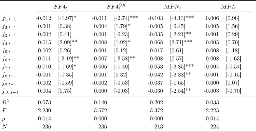
F F4t F F4GKt M P Nt M P It

f1,t−1 -0.012 [-1.97]* -0.011 [-2.74]*** -0.103 [-4.13]*** 0.006 [0.98]

f2,t−1 0.001 [0.38] 0.004 [1.79]* -0.005 [-0.45] 0.005 [1.56]

f3,t−1 0.002 [0.41] -0.001 [-0.23] -0.035 [-2.21]** 0.001 [0.29] f4,t−1 0.015 [2.09]** 0.008 [1.92]* 0.068 [2.71]*** 0.005 [0.70]

f5,t−1 0.002 [0.26] 0.001 [0.12] 0.017 [0.61] 0.008 [1.18]

f6,t−1 -0.011 [-2.19]** -0.007 [-2.58]** 0.008 [0.57] -0.008 [-1.63] f7,t−1 -0.010 [-1.69]* -0.006 [-1.40] -0.053 [-2.85]*** -0.004 [-0.54] f8,t−1 -0.001 [-0.35] 0.001 [0.32] -0.042 [-2.38]** -0.001 [-0.15] f9,t−1 -0.002 [-0.59] -0.002 [-0.53] -0.037 [-1.65] 0.000 [0.07] f10,t−1 0.004 [0.75] 0.000 [-0.03] -0.030 [-2.54]** -0.003 [-0.70]

R2 _{0.073 0.140 0.202 0.033}

F 2.230 3.572 3.372 2.225

p 0.014 0.000 0.000 0.014

N 236 236 213 224

Note: Regressions include a constant and 1 lag of the dependent variable. 1990:2009. From left to right, the monthly surprise in the fourth federal funds future (F F4t), the instrument in Gertler and Karadi

(2015) (F F4GKt ), the narrative series of Romer and Romer (2004) (M P Nt), and the informationally

robust instrument constructed in Section1.3(M P It). The ten dynamic factors are extracted from the

set of monthly variables inMcCracken and Ng (2015). t-statistics are reported in square brackets, *

p <0.1, **p <0.05, *** p <0.01, robust standard errors.

anticipated changes in the economic outlook.

Operationally, we proceed in three steps. First, we build monthly surprises (F F4t

discussed above) as the sum of the daily series inG¨urkaynak, Sack and Swanson(2005).

These are the price revisions in interest rates futures that are registered following FOMC

announcements. The daily series used to construct the monthly monetary policy

sur-prises (mpst) are the intraday movements in the fourth federal funds futures contracts

that are registered within a 30-minute window surrounding the time of the FOMC

an-nouncements. These contracts have an average maturity of about three months. Federal

funds futures settle based on the average effective federal funds rate prevailing on the

expiry month, their price can therefore be thought of as embedding markets’ forecasts

about future policy rates. Under the assumption of a constant risk premium, a price

of policy that is unexpected by market participants, given their pre-announcement

in-formation set. This is the assumption made in e.g. G¨urkaynak et al. (2005). We think

of these series of monthly surprises as a proxy for the revisions in expectations in the

aggregate economy that are triggered by central bank’s policy decisions. Second, we

regress these monthly surprises onto (i) their lags, to mod out the autocorrelation due

to the slow absorption of information; and (ii) followingRomer and Romer(2004), onto

Greenbook forecasts and forecast revisions for real output growth, inflation and the

unemployment rate, to control for the central bank’s private information.

Specifically, we recover an instrument for monetary policy shocks using the residuals

of the following regression:

mpst= α0+

p

X

i=1

αimpst−i+

+

3

X

j=−1

θjFtcbxq+j+

2

X

j=−1

ϑj

F_tcbxq+j−Ftcb−1xq+j

+ zt. (16)

mpst denotes the monetary surprise that follows the FOMC announcements in montht.

Fcb

t xq+j denotes Greenbook forecasts for quarterq+j made at time t, where q denotes

the current quarter. F_tcbxq+j −Ftcb−1xq+j

is the revised forecast for xq+j between two

consecutive meetings. For each surprise, the latest available forecast is used. xq includes

output, inflation, and unemployment.16

In Figure 2 we plot the original monetary surprise mpst (F F4t, orange line) and

our instrument for the monetary policy shock zt (M P It, blue line). Despite the many,

obvious similarities between the two series, the chart shows that significant discrepancies

arise particularly during times of economic distress (see Figure C.1 in Appendix C).

Most importantly, however, the difference between these two series is in the numbers in

Table 3, where the rightmost columns report the results of the test for the presence of

informational frictions inzt (M P It). Consistent with our prior, we do not find evidence

of predictability for our instrument given past information.

16_{FollowingRomer and Romer(2004) we only include the nowcast for the level of the unemployment}

Figure 2: Informationally-robust instrument for monetary policy shocks

Chair Bernanke

percentage points

1992 1994 1996 1998 2000 2002 2004 2006 2008 −0.4

−0.2 0 0.2

Market−Based Surprise FF4

t

Monetary Policy Instrument MPI

t

Note: market-based surprises conditional on private agents’ information setF F4t(orange line), residual

to Eq. (16)M P It(blue, solid). Shaded areas denote NBER recessions.

2

Transmission

Correct inference of the dynamic effects of monetary policy shocks hinges on the

in-teraction between the identification strategy and the modelling choice. Modern

mac-roeconomics thinks of the residuals of autoregressive models as structural stochastic

innovations – combinations of economically meaningful shocks –, and identifies the ones

of interest using theory-based assumptions, and often external instruments. Once

struc-tural shocks are meaningfully identified, the autoregressive coefficients of the model are

employed to study the transmission of the exogenous disturbances over time. Modelling

choices are therefore of great importance. First, in separating the stochastic component

of the economic processes as distinct from the autoregressive and deterministic ones.

Second, in providing a reduced-form description of the propagation of identified shocks

over time.

Time series econometrics has provided applied researchers with results that prove

the consistency of estimates under the quite restrictive assumption that the model

cor-rectly captures the data generating process (DGP). However, it is well understood that

para-meters – transmission coefficients and covariance matrix alike – are inconsistent (Braun and Mittnik, 1993). This affects the identification of the disturbances, the variance-covariance decomposition, and the derived impulse response functions (IRFs). These

concerns have motivated the adoption of more flexible, ‘non-parametric’ empirical

spe-cifications, such as Jord`a (2005)’s local projections (LP).

VARs produce IRFs by iterating up to the relevant horizon the coefficients of a

one-step-ahead model. Hence, if the one-step-ahead VAR is misspecified, the resulting

errors are compounded at each horizon in the estimated IRFs. Conversely, the local

projection method estimates impulse response functions from the coefficients of direct

projections of variables onto their lags at the relevant horizon. This makes LP more

robust to a number of model misspecifications, and thus a theoretically preferable choice.

In practice, however, the theoretical appeal of LPs has to be balanced against the

large estimation uncertainty that surrounds the coefficients’ estimates. From a classical

perspective, one faces a sharp bias-variance trade-off when selecting between VARs and

LPs.

In what follows, we review the two methods, and propose a Bayesian approach to

Local Projections (BLPs) as an efficient way to bridge between the two, by mean of

informative priors. Intuitively, we propose a regularisation for LP-based IRFs which

builds on the prior that a VAR can provide, in first approximation, a decent description

of the behaviour of most macroeconomic and financial variables. As the horizon grows,

however, BLP are allowed to optimally deviate from the restrictive shape of VAR-based

IRFs, whenever these are poorly supported by the data. This while the discipline

imposed by our prior allows to retain reasonable estimation uncertainty at all horizons.

2.1

Recursive VARs and Direct LPs

The standard practice in empirical macroeconomics is to fit a linear vector autoregression

to a limited set of variables. This in order to retrieve their moving average

VAR can be written in structural form as

A0yt+1 = K +A1yt+. . .+Apyt−(p−1)+ut+1 , (17)

ut ∼ N(0,Σu) ,

where t=p+ 1, . . . , T, yt = (yt1, . . . , ynt)0 is a (n×1) random vector of macroeconomic

variables,Ai,i= 0, . . . , p, are (n×n) coefficient matrices (the ‘transmission coefficients’),

and ut = (u1t, . . . , unt)0 is an n-dimensional vector of structural shocks. It is generally

assumed that Σu =In. VARs are estimated in reduced form, i.e.

yt+1 =C+B1yt+...+Bpyt−(p−1)+εt+1 , (18)

εt ∼ N(0,Σε),

where εt=A−01ut, E[εtε0t] =A

−1 0 (A

−1 0 )

0 _{= Σ}

ε, and Bi =A−01Ai. C =A−01K.

Given A0, the IRFs to the identified structural shocks can be recursively computed

for any horizonh as

IRFVAR_h =

h

X

j=1

IRFVAR_h−jBj , (19)

where IRFVAR₀ =A−₀1 and Bj = 0 forj > p. IRFVARh is an (n×n) matrix whose element

(i, j) represents the response of variable i to the structural shock j, h periods into the

future.

Despite being a workhorse of empirical macroeconomics, VARs are likely to be

mis-specified along several dimensions. First, the information set incorporated in a small-size

VAR can fail to capture all of the dynamic interactions that are relevant to the

propaga-tion of the shock of interest. For example, Caldara and Herbst (2016) argue that the

failure to account for the endogenous reaction of monetary policy to credit spreads

in-duces a bias in the shape of the response of all variables to monetary shocks. More

generally, there is evidence that policy makers and private agents are likely to assess

a large number of indicators when forming expectations and taking decisions (see, for

of the underlying process may potentially be underestimated. Also, if the disturbances

of the underlying DGP are a moving average process, fitting a low-order, or indeed any

finite-order VAR may be inadequate.17 _{Finally, several possible non-linearities of}

differ-ent nature may be empirically significant – such as time-variation or state-dependency

of some of the parameters, and non-negligible higher order terms. In this

perspect-ive, to empirically pin down all of the different sources of misspecification in order to

parametrise them in a model is almost a self defeating effort.

As an alternative to the recursive VAR impulse response functions, the local

projec-tions (LP) `a la Jord`a(2005) estimate the IRFs directly from the linear regression

yt+h =C(h)+B

(h)

1 yt+...+B

(h) ˜

p yt−( ˜p+1)+ε (h)

t+h , (20)

ε(_th₊)_h ∼ N(0,Σ(_εh)) ∀ h= 1, . . . , H ,

where the lag order ˜p may depend on h. The residuals ε(_th₊)_h, being a combination of

one-step-ahead forecast errors, are serially correlated and heteroskedastic. Given A0,

the structural impulse responses are

IRFLP_h =B₁(h)A−₀1 . (21)

In the forecasting literature, the distinction between VAR-based recursive IRFs and

LP-based direct IRFs corresponds to the difference between direct and iterated forecasts (see

Marcellino, Stock and Watson, 2006;Pesaran, Pick and Timmermann, 2011;Chevillon,

2007, amongst others). An implicit assumption of both the approaches is that

macroeco-nomic and financial time series possess either approximately linear, or only moderately

nonlinear behaviour that can be captured by a linear model, in first approximation.

This assumption is supported by a wealth of empirical evidence, amongst all the well

established fact that factor models are able to summarise and produce decent forecasts

of large panels of macroeconomic variables, due to their underlying approximated factor

structure.

17_{If the process is stationary, there exists an infinite moving average representation of it (the Wold}

If a VAR correctly captures the DGP, its recursively generated IRFs are both optimal

in mean square sense, and consistent. Because it is implausible that typically low-order

autoregressive models be correctly specified, the robustness of LP responses to model

misspecification makes them a more attractive procedure compared to the bias-prone

VAR.18 _{However, due to the moving average structure of the residuals, and the risk of}

over parametrisation, local projections are likely to be less efficient, and hence subject

to volatile and imprecise estimates (see, for example, the discussion in Ramey, 2013).

In fact, empirical studies indicate that the potential gains from direct methods are

not always realised in practice. Comparing direct and iterated forecasts for a large

collection of US variables of given sample length, Marcellino, Stock and Watson (2006)

note that iterated forecasts tend to have, for many economic variables, lower sample

MSFEs than direct forecasts. Also, direct forecasts become increasingly less desirable

as the forecast horizon lengthens. Similarly, comparing the finite-sample performance

of impulse response confidence intervals based on local projections and VAR models in

linear stationary settings,Kilian and Kim (2011) find that asymptotic LP intervals are

often less accurate than the bias-adjusted VAR bootstrapped intervals, notwithstanding

their large average width. Hence, from a classical perspective, choosing between iterated

and direct methods involves a sharp trade-off between bias and estimation variance: the

iterated method produces more efficient parameters estimates than the direct method,

but it is prone to bias if the one-step-ahead model is misspecified.

2.2

Bayesian Local Projections

From a Bayesian perspective, the trade-off between bias and variance involved in the

choice between iterated VAR-IRFs and direct LPs-IRFs is a natural one. This is also true

for classical ‘regularised’ regressions, providing an alternative frequentist interpretation

of Bayesian techniques (see, for example,Chiuso, 2015). Moving from this observation,

we design a new flexible linear method that bridges between iterated VAR responses

18_{In a simulated environment, and with regard to multi-step forecasts,Schorfheide(2005) shows that}

and direct local projections. We refer to this new method as Bayesian Local Projection

(BLP). Alternatively, we could speak of ‘regularised Local Projections’.

The mapping between VAR coefficients and LP coefficients provides a natural way to

inform Bayesian priors about the latter (or to regularise the regression), hence essentially

spanning the space between iterated and direct response functions. To provide the gist

of our approach, let us consider the AR(1) specification of (19) and (20) – i.e. their

companion form. Forh= 1, both models reduce to a standard VAR(1)

yt+1 =C+Byt+εt+1 . (22)

Iterating the VAR forward up to horizon h, we obtain

yt+h = (I−B)−1(I−Bh)C+Bhyt+ h

X

j=1

Bh−jεt+j (23)

= C(VAR,h)+B(VAR,h)yt+ε

(VAR,h)

t+h . (24)

Coefficients and residuals can now be readily mapped into those of a LP regression in

companion form

yt+h =C(h)+B(h)yt+ε

(h)

t+h , (25)

obtaining

C(h) ←→C(VAR,h) = (I−B)−1(I−Bh)C , (26)

B(h) ←→B(VAR,h)=Bh , (27)

ε(_th₊)_h ←→ε(VAR_t+h ,h) =

h

X

j=1

Bh−jεt+h . (28)

The impulse response functions are given by Eq. (27), up to the identification matrix

A0 (and a selection matrix for the companion form):

IRFVAR_h =BhA−₀1 , (29)

Three observations are in order. First, conditional on the underlying data generating

process being the linear model in Eq. (22), and abstracting from estimation uncertainty,

the IRFs computed with the two different methods should coincide. Second, as shown

by Eq. (28), conditional on the linear model being correctly specified, LPs are bound

to have higher estimation variance due to (strongly) autocorrelated residuals.19 _Third,

given that for h = 1 VARs and LPs coincide, the identification problem is identical

for the two methods. In other words, given an external instrument or a set of

theory-based assumptions, the way in which theA0 matrix is derived from either VARs or LPs

coincides.

The map in Eq. (26-28) provides a natural bridge between the two empirical

spe-cifications that can be used to inform priors for the LP coefficients used to estimate

the IRFs at each horizon. Clearly, if we believed the VAR(p) to be the correct

specific-ation, then LP regressions would have to be specified as ARMA(p, h−1) regressions.

Their coefficients could be then estimated by combining informative priors with a fully

specified likelihood (see Chan et al., 2016). If, however, the VAR(p) were to effectively

capture the DGP, it would be wise to discard direct methods altogether. More

gener-ally, if we were to know the exact source of misspecification of any given VAR(p), we

could draw inference from a fully parametrised, correctly specified model. However, this

is not possible in practice. An alternative, robust approach to the strong parametric

assumptions that are typical of Bayesian VAR inference is the adoption of a misspecified

likelihood function to conduct inference about the pseudo-true parameters of interest,

as proposed in M¨uller (2013).

2.3

Informative Priors for LPs

For the coefficients of Eq. (20) at each horizonh, and leaving temporarily aside concerns

about the structure of the projection residuals, we specify standard conjugate

Normal-19_{Most macroeconomic variables are close to I(1) and even I(2) processes. Hence LP residuals are}

inverse Wishart informative priors of the form

Σ_ε(h) |γ ∼ IWΨ₀(h), d(₀h) ,

β(h) | Σ_ε(h), γ ∼ N β₀(h),Σ_ε(h)⊗Ω₀(h)(γ) , (31)

where β(h) _{≡ vec(b}(h)_{) = vec}

h

C(h)_{, B}(h)

1 , . . . , B (h) ˜

p

i0

is the vector containing all the

local projection coefficients at horizon h. We use β₀(h) to denote the prior mean, and γ

for the generic vector collecting all the priors’ hyperparameters.

As in Kadiyala and Karlsson (1997), we set the degrees of freedom of the

inverse-Wishart distribution tod(₀h)=n+2, the minimum value that guarantees the existence of

the prior mean for Σ(εh), equal to Ψ(0h)/(d (h)

0 −n−1). As is standard in the macroeconomic

literature, we use sample information to fix some some of the hyperparameters of the

prior beliefs. In particular, at each horizon we set the prior scale Ψ(₀h) to be equal to

Ψ(₀h)=diagh(σ₁(h))2, . . . ,(σ_n(h))2i ,

where (σ_i(h))2 are the HAC-corrected variances of the autocorrelated univariate local

projection residuals. Similarly, we set Ω(₀h) as

Ω(₀h)(γ)

(np˜+1×np˜+1)

= 

 

−1 0

0 _Ip˜⊗(λ(h))2diag

h

(σ₁(h))2, . . . ,(σn(h))2

i−1





,

where we take to be a very small number, thus imposing a very diffuse prior on the

intercepts. One single hyperparameter, λ(h), controls the overall tightness of the priors

at each horizonh, i.e. γ ≡λ(h)_.

specification implies the following first and second moments for the IRF coefficients

E

h

B_ij(h) |Σ_ε(h)i =B(₀h_,ij), (32)

Var

h

B_ij(h) |Σ(_εh) i

= (λ(h))2(σ

(h)

i )2

(σ(_jh))2, (33)

where B_ij(h) denotes the response of variable i to shock j at horizon h, and B₀(h) is such

that β₀(h) =vec(B₀(h)).

There are many possible ways to inform the prior meanβ₀(h). Our preferred one is to

set it to be equal to the posterior mean of the coefficients of a VAR(p) iterated at horizon

h. The VAR used to inform the BLP prior is estimated with standard macroeconomic

priors over a pre-sampleT0, that is then discarded.20 In the notation of model (22) this

translates into

β₀(h) =vec(B_Th₀), (34)

where Bh

T0 is the h-th power of the autoregressive coefficients estimated over the

pre-sample. Intuitively, the prior gives weight to the belief that a VAR can describe the

behaviour of economic time series, at least first approximation.

Having not explicitly modelled the autocorrelation of the residuals has two important

implications. First, the priors are conjugate, hence the posterior distribution is of the

same Normal inverse-Wishart family as the prior probability distribution. Second, the

Kronecker structure of the standard macroeconomic priors is preserved. These two

important properties make the estimation analytically and computationally tractable.

Conditional on the observed data, the posterior distribution takes the following form

Σ(_εh) | γ(h),y∼ IW Ψ(h), d

β(h) | Σ_ε(h), γ(h),y ∼ Nβ˜(h),Σ_ε(h)⊗Ω(h) , (35)

20_{An obvious alternative is the generalisation of the standard macroeconomic priors proposed in} Litterman (1986), centred around the assumption that each variable follows a random walk process, possibly with drift. Results using this alternative prior are discussed in Section 3. Also, one could specify a hyperprior distribution for the first autocorrelation coefficients, as a generalisation ofLitterman

where d=d(₀h)+T, and T is the sample size.

Because of the structure of the residuals, however, this parametrisation is

misspe-cified. The shape of the true likelihood is asymptotically Gaussian and centred at the

Maximum Likelihood Estimator (MLE), but has a different (larger) variance than the

asymptotically normal sampling distribution of the MLE in Eq. (35). This implies

that if one were to draw inference about β(h) – i.e. the horizon-h responses –, from the

misspecified likelihood in Eq. (35), one would be underestimating the variance albeit

correctly capturing the mean of the distribution of the regression coefficients. M¨uller

(2013) shows that posterior beliefs constructed from a misspecified likelihood such as

the one discussed here are ‘unreasonable’, in the sense that they lead to inadmissible

decisions about the pseudo-true values, and proposes a superior mode of inference –

i.e. of asymptotically uniformly lower risk –, based on artificial ‘sandwich’ posteriors.21

Hence, in line with the classical practice, we conduct inference about β(h) _{by replacing}

the original posterior with an artificial Gaussian posterior centred at the MLE but with

a HAC-corrected covariance matrix. This allows us to remain agnostic about the source

of model misspecification as in Jord`a (2005). Specifically, following M¨uller (2013), we

replace Eq. (35) with an artificial likelihood defined as

Σ(_ε,h_HAC) | γ(h),y∼ IWΨ(_HACh) , d

,

β(h) | Σ_ε,(h_HAC) , γ(h),y ∼ Nβ˜(h),Σ_ε,(h_HAC) ⊗Ω(h). (36)

Lastly, it is worth noting that by specifyingβ₀(h) as in Eq. (34), BLP IRFs effectively

span the space between VARs and local projections. To see this, note that given the

prior in (31), the posterior mean of BLP responses takes the form

B_BLP(h) ∝

X0X+

Ω(₀h)(γ)

−1−1

X0Y(h)+

Ω(₀h)(γ) −1

B_VARh

, (37)

where B(_BLPh) is such that ˜β(h) _{= vec(B}(h)

BLP). (X

0_X)−1_(X0_Y(h)_{) = B}(h)

LP, where Y(h) ≡

21_{For the purpose of this work, the ‘decisions’ concern the description of uncertainty around β}(h)

(yp+1+h, . . . , yT)0, X ≡ (xp+1+h, . . . , xT)0, and xt ≡(1, yt0−h, . . . , y

0

t−(p+h))

0_{. At each}

hori-zon h, the optimal combination between VAR and LP responses is regulated by Ω(₀h)(γ)

and is a function of the overall level of informativeness of the priorλ(h)_{. Whenλ}(h) _→0,

BLP IRFs collapse into VAR IRFs (estimated over T0). Conversely, if λ(h) → ∞ BLP

IRFs coincide with those implied by standard LP.

2.4

Optimal Priors

In our model, the informativeness of the priors is controlled by the hyperparameterλ(h)

that regulates the covariance matrix of all the entries inβ(h) _{at horizonh. We treatλ}(h)

as an additional model parameter, for which we specify a prior distribution, or hyperprior

p(λ(h)_{), and estimate it at each h in the spirit of hierarchical modelling. As observed}

in Giannone et al. (2015), the choice of the informativeness of the prior distribution is conceptually identical to conducting inference on any other unknown parameter of the

model. As such, the hyperparameters can be estimated by evaluating their posterior

distribution, conditional on the data

p(λ(h)|y(h)_{) =p(y}(h)_|λ(h)_)·p(λ(h)_{) , (38)}

wherep(y(h)|λ(h)) is the marginal density of the data as a function of the

hyperparamet-ers, and y(h) _=vec(Y(h)_{). Under a flat hyperprior, the procedure corresponds to}

max-imising the marginal data density (or marginal likelihood, ML), which can be thought

of as a measure of the forecasting performance of a model.22

Extending the argument in Giannone et al. (2015) we write the ML as

p(y(h)|λ(h))∝

V

posterior ε(h)

−1

V_εp(hrior)

T−( ˜p+h)+d

2

| {z }

Fit

T−h

Y

t= ˜p+1

V_t+h|t

−1 2

| {z }

Penalty

∀h , (39)

where V_εp(hosterior) and V prior

ε(h) are the posterior and prior mean of Σ

(h)

ε , and Vt+h|t =

22_{As discussed inGiannone et al.(2015), estimating the hyperparameters by maximising the ML –}

E_Σ(h)

ε h

Var(yt+h|yt,Σ(εh))

i

is the variance (conditional on Σ(εh)) of the h-step-ahead

fore-cast ofy, averaged across all possible a priori realisations of Σ(εh).23 The first term in Eq.

(39) relates to the model’s in-sample fit, and it increases when the posterior residual

variance falls relative to the prior variance. The second term is related to the model’s

(pseudo) out-of-sample forecasting performance, and it increases in the risk of

overfit-ting (i.e. with either large uncertainty around parameters’ estimates, or large a-priori

residual variance). Thus, everything else equal, the ML criterion favours

hyperparamet-ers values that generate both smaller forecast errors, and low forecast error variance,

therefore essentially balancing the trade-off between model fit and variance.

Empirically, the optimal level of informativeness of BLP priors may depend, amongst

other characteristics of the data, on the size of the time series, the level of noise, and the

degree of misspecification of the VAR. However, it is natural to expect that deviations

from the VAR will be smaller for smallerh, where the compounded effect of the potential

misspecifications is relatively milder. Consistent with this intuition, to set λ(h) _we

choose from a family of Gamma distributions and let the hyperprior be more diffuse

the higher the forecast horizon (or projection lag). In particular, we fix the scale and

shape parameters such that the mode of the Gamma distribution is equal to 0.4, and

the standard deviation is a logistic function of the horizon that reaches its maximum

afterh= 36. Figures B.1aand B.1b in the Appendix provide details.

3

VAR, LP, and BLP

We start our empirical exploration by comparing the IRFs estimated using the three

methods discussed in the previous section – VAR, LP, and BLP (Figure3). The matrix

of contemporaneous transmission coefficients A0 is the same in the three cases (recall

that forh= 1 BLP and the VAR coincide. See Section2.2.) and is estimated using our

informationally robust series M P It as an external instrument.24 The contractionary

23_{The derivation of this formula follows as in the online Appendix ofGiannone et al.(2015).} 24_{Specifically, ifu}

tandξtdenote, respectively, the monetary policy shock and the vector of all other

shocks, the identifying assumptions are