ISSN: 1816-949X
© Medwell Journals, 2020
Selection of Tuning Parameter in L1-Support Vector Machine via.
Particle Swarm Optimization Method
1
Niam Abdulmunim Al-Thanoon,
2Omar Saber Qasim and
3Zakariya Yahya Algamal
1Department of Operations Research and Artificial Intelligence,
2
Department of Mathematics,
3
Department of Statistics and Informatics, University of Mosul, Mosul, Iraq
Abstract: Descriptor selection for classification methods is one of the most important topics in the chemometrics. The selection of descriptors can be considered to be a variable selection problem that aims to find a small subset of descriptors that has the most discriminative information for the classification target. Penalized Support Vector Machine (PSVM) is one of the most effective embedded methods and it is more preferable than the Support Vector Machine (SVM) because PSVM combines the standard SVM with a penalty to simultaneously perform both variable selection and classification. The PSVM with L1-norm is the most widely used methods. However, the efficiency of PSVM with L1-norm depends on appropriately choosing the tuning parameter which is involved in the L1-norm penalty. In this study, a particle swarm optimization method which is a metaheuristic continuous algorithm is proposed to determine the tuning parameter in PSVM with L1-norm penalty. The proposed method will efficiently help to find the most significant descriptors in constructing Quantitative Structure–Activity Relationship classification (QSAR) model with high classification performance. Depend on the four datasets, the experimental results show the favorable performance of the proposed method when the number of descriptors is high and the sample size is low comparing with other competitor methods.
Key words:QSAR, L1-norm, classification, penalized support vector machine, particle swarm optimization, cluster
INTRODUCTION
With the development of technologies in the chemometrics, large volumes of chemical data are generated, presenting a challenge for chemometricians to conduct the statistical classification. One of these challenges is the low number of observations (chemical compounds) and the large number of variables (descriptors) (Al Fakih et al., 2016). High dimensionality of the data affects the performance of any used classifier due to the presence of irrelevant, noisy and redundant variables. These uninformative variables may dominate the informative variables for classification.
Variable selection which is also known as dimensionality reduction is the method of selecting an optimum subset of relevant variables that can improve the performance of statistical classification and to avoid the curse of dimensionality (Khajeh et al., 2012). Consequently, several variable selection methods have been proposed and studied in the literature. These methods can be divided into three broad categories: The filter, wrapper and embedded methods (Algamal and Lee, 2015).
Filter methods are one of the most popular variable selection methods which are based on a specific criterion by gaining information of the each variable. These methods are work separately and they are not dependent
on the classification method. For the wrapper methods, on the other hand, the variable selection process is based on the performance of a classification algorithm to optimize the classification performance. In embedded methods, variable selection process is incorporated into the classification methods which can simultaneously perform variable selection and classification (Liang et al., 2013). Support Vector Machine (SVM) has attracted much substantial attention from many statisticians in recent years because of its theoretical and practical advantages that justify its improved performance in classification (Shen et al., 2007). The main objective of the SVM is to find a hyper-plane which effectively separates between two classes of data points to identify a decision boundary with the maximum geometric margin (Cong et al., 2013). Despite the excellent characteristics of SVM, there are still several drawbacks including the selection of variables. In other words, SVM cannot perform variable selection (Zhu et al., 2004). Penalized Support Vector Machine (PSVM) which is one of the most effective embedded methods is more preferable than the SVM because PSVM combines the standard SVM with a penalty to simultaneously perform both variable selection and classification (Wang et al., 2008). With deferent penalties, numerous PSVMs can be applied, among them is L1-norm which is known as the least absolute shrinkage and selection operator (lasso) (Broman and Speed, 2002).
However, the efficiency of PSVM with L1-norm depends on appropriately choosing the tuning parameter which is involved in the L1-norm penalty. The tuning parameter controls the tradeoff between classification and the number of selected variables. As a result, selecting a suitable value of the tuning parameter is an important part of fitting. The most widely used approach for selecting the tuning parameter is Cross-validation (CV) which is a data-driven approach. However, it was pointed out that CV usually identify too many irrelevant variables when the number of variables is large and can be very time consuming (Park et al., 2014).
In this study, a particle swarm optimization method which is a metaheuristic continuous algorithm is proposed to determine the tuning parameter in PSVM with L1-norm penalty. The proposed method will efficiently help to find the most significant variables in constructing quantitative structure-activity relationship classification model with high classification performance. The experimental results show the favorable performance of the proposed method when the number of variables is high and the sample size is low.
MATERIALS AND METHODS
Support vector machine: Support vector machine is an excellent, efficient, effective and a powerful classification method for binary classification problems which is based on the statistical learning theory (Dong and Jian, 2015).
Support vector machine has several important advantages: great flexibility, high accuracy, ability of generalization, computational efficiency, high performance when the number of variables is large and dealing with complex nonlinear problems using a simple linear algorithm by using soft margin approach (Bi et al., 2003). Training SVM is equivalent to solving the problem of convex linear constrained quadratic programming. SVM is based on mapping the sample observations into a high-dimensional feature space to search and obtain an optimal separating hyperplane which maximizes the sum of the distances between two classes in this space (Liu et al., 2010).
In chemometrics application, descriptor matrix can be described as a matrix X = (xij)n×d where each column
represents a descriptor and each row represents a sample (compound). The numerical value of xij denotes the value of a specific descriptor J (j = 1,…, d) in a specific sample i( = 1,…, n). For a binary classification problem, given a training dataset n where, xi = (xi,j, xi,2,…, xi,d)
i i i 1
{(x , y )}
represents a vector of the ith descriptor and ti0{-1,
+1} for i = 1,…, n where, yi = +1 indicates the ith sample
is in class 1 and yi = -1 indicates the ith sample is in class 2.
An SVM generates a real-valued function n(X) as a hyperplane to maximize the distance, w, between the data which should be separated. There exists two parallel boundaries n(X).w+b = K1 which can exactly separate two classes. The separating hyperplane, sgn(n(x).w+b), is between them. The margin between these two boundaries is defined as 2/||w||. In order to maximize this margin, the following problem must be solved as:
(1) T
w,b
i i i
1 min w w
2
S.T. y ( (x ) w b) 1, i1, 2,..., n.
By solving this problem, the optimal hyperplane of Eq. 1 with a solution of and are
sgn((w x) b) w b
obtained.
Depending on Lagrangian, Eq. (1) can be written as a quadratic dual optimization problem by:
(2)
n n n
T i j i j i j i
i 1 j 1 i 1
n
i i i
i 1
S 1
min y y x x 2
y 0, 0 , i 1, 2, ..., n .T.
Where:
α : A vector of Lagrange multipliers vector αi : Corresponds to a training observation (xi, yi)
Equation 1 and 2 are used for linearly separable training observations. However, to extend the SVM for the linearly non-separable training observations, each observation (xi, yi) is associated with a slack variable ζi>0.
The constraint in Eq. 1 becomes yi(n(xi)wi+b)+ζi>0. Thus Eq. 1 becomes:
(3) n
T
i
w, b i 1
i i i i
1 min w w C
2
S.T. y ( (x ) w b) 1, i 1, 2, ..., n
where C is a parameter that controls the tradeoff between the maximum margin and the minimum classification error. Then, the Lagrangian becomes:
(4)
n n n
i j i j i j i
i 1 j 1 i 1
n
i i i
i 1
K( . )
S. 1
min y y x x 2
y 0, 0 C , i 1, 2, n
T. ...,
where, K(xi.xj) = n(xi) Tn(x
j) is the kernel function that
Penalized support vector machine: Although SVM has been proven useful in binary classification, it cannot perform features selection because of using L2-norm, . Typically, any classification problem includes a 2
2
|| w ||
number of features where many of these features can be noisy or redundant, leading to degrade the performance of the classification algorithm. Therefore, reducing dimensions is an essential step that can be achieved through feature selection strategies.
Bradley and Mangasarian (1998) and Zhu et al. (2004) proved that the SVM optimization problem is equivalent to a penalization problem which has the form:
(5)
n
i i w , b i 1
1
min 1 y f (x ) Pen (w)
n
where, [1-yi f(xi)]+ = max(1-yi f(xi), 0) represents the hinge loss term and Penλ (w) represents the penalty term. Several penalties have been proposed. Among them, L1-norm (Zhu et al.. 2014; Bradley and Mangasarian, 1998), Lq-norm with q<1 (Liu et al., 2010; Ikeda and Murata, 2005; Liu et al., 2007). Furthermore, Zhang, et al. (2005) proposed the Smoothly Clipped Absolute Deviation (SCAD) penalty of Fan and Li (2001) with SVM. In addition, Wang, et al. (2008) proposed a hybrid huberized SVM by using the elastic net penalty while Becker, et al. (2011) proposed a combination of ridge and SCAD with SVM.
The L1-norm penalty, proposed by Bradley and Mangasarian (1998) and Zhu et al. (2004) is one of the most popular penalty function because SVM with L1-norm can automatically select features by shrinking the hyper-plane coefficients to zero. The SVM-L1 is defined as:
(6)
n d
i i j
w , b
i 1 j 1
1
min 1 y f (x ) | w |
n
where, λ is a positive tuning parameter which controls the amount of shrinkage. Equation 6 is a convex optimization problem and can be solved by the method of Lagrange multipliers.
Particle swarm optimization method: Particle Swarm Optimization (PSO) is a nature-inspired metaheuristic algorithm that was originally proposed by Kennedy and Eberhart (1995) for solving continuous optimization problems.
The PSO inspires the social or collective behavior of animals such as bird flocking and fish schooling. PSO compares with the other computation intelligence-based algorithms has several advantages such as simple
implementation, computationally higher efficiency, fewer parameters to tune, scalability and flexibility, robustness. For instance, comparing with genetic algorithm, there is no crossover and mutation genetic operation (Chen et al., 2014; Kiran, 2017; Lin et al., 2008; Lu et al., 2011; Zhou and Dickerson, 2014).
The PSO performs the searching using a population which is called swarm, of particles. Each particle has three features: position, velocity and fitness value. In PSO, each particle can be represented as a candidate solution (position) in the search space. The particles fly through the search space by their own efforts and in cooperation with other particles and they follow the best solutions they have achieved (local best solutions) as well as tracking the best solutions that they found (the best global solution) (Cervantes et al., 2017; Lai et al., 2016; Mirjalili and Lewis, 2013; Wen et al., 2011).
Mathematically, the search space is assumed to be D-dimensional and there are m of particles in the swarm where d = 1, 2…, D. During the movement, each particle has a position vector xi = {xi1, xi2,…, xid} with a velocity
vector vi = {vi1, vi2,…, vid}. In the PSO algorithm, the best
position which gives the best fitness value for the particle i is called best previous position denoted as Pbesti =
{Pbesti1, Pbesti2,…, Pbestid}. The best position found by
all particles is called the global best which is denoted as Gbesti = {Gbesti1, Gbesti2,…, Gbestid}. In each iteration,
the PSO algorithm searches for the optimal solution by updating the position and the velocity of the ith particle according to the following two equations:
(7)
t 1 t t t t t
id id 1 1 id id 2 2 id id
v z v c r Pbest x c r Gbest x
where, t denotes the iteration in the algorithm, z is the inertia weight which is used to balance between the global search and the local search. In addition, c1 (the cognition
learning factor) and c2 (social learning factor) are the
acceleration coefficients. While r1 and r2 are random
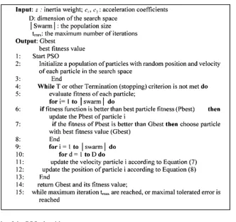
values selected from a uniform distribution with (0,1). The pseudo code of the PSO algorithm is displayed in Fig. 1.
Fig. 1: Pseudo code of the PSO algorithm
In literature, the most widely used method for selecting λ is the Cross-Validation (CV), which is a data-driven approach. However, it was pointed out that CV usually identify too many irrelevant variables when the number of variables is large (Broman et al., 2002; Chen et al., 2014) and can be very time consuming (Park et al., 2014). Consequently, several modification of the CV approach in estimating λ have been suggested by researchers (Roberts and Nowak, 2014; Sabourin et al., 2015; Jung and Hu, 2015; Meijer and Goeman, 2013; Pang et al., 2016).
Due to drawbacks of CV approach, in this study, a PSO algorithm is proposed to determine the tuning parameter in PSVM with L1-norm penalty. The proposed method will efficiently help to find the most significant variables in constructing quantitative structure-activity relationship classification model with high classification performance. The parameter configurations for our proposed method are presented as follows.
The number of particles, m is set to 50 and the number of iterations is tmax = 100. The acceleration
coefficients c1 and c2 are set within the range
(Khajeh et al., 2012; Liang et al., 2013). The c1 and c2 are
updating during the iteration according to the following equations:
(9) 1 1,min 1,max 1,min
max
t
c c (c c )
t
2 2,min 2,max 2,min max
t
c c (c c )
t
Further, the minimum and the maximum values for the inertial weight are: zmin = 0.2 and zmax = 0.9. The
inertial weight is updating according to the following equation:
max max min
max
t
z z (z z ) t
The positions of each particle are randomly determined. The position of a particle represents the tuning parameter, λ. The initial positions of the particles are generated from a uniform distribution within the range (0-100). The initial velocities of each particle are generated from a uniform distribution within the range (0, 4). The fitness function is defined as:
d q Fitness 0.8 CA 0.2
d
Table 1: Characteristics of the four used datasets
Datasets Compounds No. (n) Descriptors No. (p) Class
Dataset 1 212 2571 Active = 108/inactive = 104
Dataset 2 75 3067 inhibitor = 108/non-inhibitor = 104
Dataset 3 121 2559 31 active/90 inactive
Dataset 4 479 2322 213 active/266 weakly active
where, CA is the classification accuracy that obtained, d represents the number of descriptors in the dataset, q represents the number of the selected descriptors. The fitness function are calculated for all particles and the Pbest and Gbest vectors are determined.
The velocities and positions are updated using Eq. 7 and 8, respectively. Steps 4 and 5 are repeated until a tmax is reached.
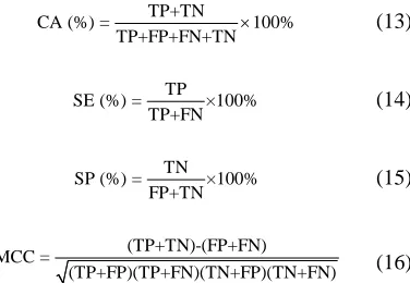
Evaluation criteria: The classification performance of the used methods was measured by Classification Accuracy (CA), Sensitivity (SE), Specificity (SP), Mathew’s Correlation Coefficient (MCC) and Area under the Curve (AUC). The used criteria are defined as:
(13)
TP+TN
= 100%
TP+FP+FN+T C
N
A (%)
(14)
TP SE (%) = ×100%
TP+FN
(15)
TN SP (%) = ×100%
FP+TN
(16)
(TP+TN)-(FP+FN) MCC =
(TP+FP)(TP+FN)(TN+FP)(TN+FN)
where TP, TN, FP and FN be the numbers of true positive, true negative, false positive and false negative of the confusion matrix, respectively. The higher value of the used evaluation criteria the power classification performance is.
Datasets: Four collected datasets that are binary classification problem and that have different numbers of descriptors and compounds are collected. Dragon Software (Version 6.0) was used to generate 4885 molecular descriptors including all 29 blocks based on the optimized molecular structures. Preprocessing steps were carried out to include consistent and useful descriptors. The first step is to discard the descriptors that had zero values. Then, remove the descriptors that had constant value for all compounds. After that, the descriptors in which 90% of their values were zeros were removed. Finally, descriptors with a relative standard deviation of <0.001 were deleted.
The four datasets are: diverse series of antimicrobial agents dataset which contains 212 different agents
with 2571 descriptors. The corresponding antimicrobial activities were measured as pMIC (the logarithm of reciprocal of minimum inhibitory) concentration against CA. The median (ME) of all 212 pMICs (ME = 1.3) as a cutoff value to classify these antimicrobial agents into active (>1.3, n=108) or inactive (<1.3, n = 104) is considered as in Daszykowski et al. (2004) and Xing et al. (2014). This dataset consists of 75 compounds with HDAC8 inhibitory activity and 3067 descriptors. According to the IC50 (half maximal inhibitory
concentration) values, the compounds are divided into two classes: An inhibitor class (0.008 μM <IC50<0.3 μM)
containing 38 compounds and a non-inhibitor class (IC50>0.3 μM) containing 37 compounds (Cao et al., 2015). A dataset of 121 molecules of thiourea derivatives with anti-HCV activity and 2559 descriptors was used by Algamal et al. (2017). According to their experimental EC50 (the concentration of a drug that gives half-maximal response), the molecules were divided into two categories by the threshold value of 0.1 μM: actives (EC50<0.1 μM)
and inactives (EC50>0.1 μM). This dataset measures 2322
descriptors corresponding to 479 neuraminidase inhibitors of in uenza a viruses (H1N1). The compounds were separated into two groups according to their IC50: active
compounds with IC50<20 μM and those with IC50>20 μM
were considered as weakly active compounds (Algamal and Lee, 2015; Li et al., 2016). The main characteristics of four datasets are summarized in Table 1.
RESULTS AND DISCUSSION
With the aim of correctly assessing the performance of our proposed method, PSVM-PSO, comparative experiments with the original CV of estimating the tuning parameter (PSVM-CV) and the modified CV of Jung and Hu (2015) (PSVM-MCV) were carried out.
In these experiments, a 10-fold is set and the range of the tuning parameters for the used methods is fixed with 0 and 100. In addition, the linear kernel function is employed. To obtain a reliable classification performance, for each dataset, a 70% of samples is used as a training dataset and remaining 20% of the samples is used as a testing dataset. This partition repeated 20 times and the averaged evaluation criteria are reported in Table 2.
Table 2: Classification performance (on average) of the methods used over 20 partitions. The number in parentheses is the standard error
Training dataset Testing dataset
Datasets Methods Selected descriptors (No.) CA SE SP MCC CA
Dataset 1 PSVM-PSO 48 (0.087) 97.04 (0.038) 96.52 (0.032) 95.80 (0.035) 0.964 (0.037) 94.83 (0.041)
PSVM-MCV 57 (1.02) 92.22 (0.371) 90.92 (0.374) 91.31 (0.372) 0.915 (0.371) 89.07 (0.411)
PSVM-CV 73 (1.11) 90.35 (0.381) 90.51 (0.387) 90.31 (0.375) 0.901 (0.382) 87.57 (0.408)
Dataset 2 PSVM-PSO 31 (0.117) 96.22 (0.121) 94.74 (0.124) 93.68 (0.123) 0.958 (0.121) 93.21 (0.217)
PSVM-MCV 49 (0.741) 92.72 (0.214) 91.12 (0.236) 91.36 (0.242) 0.918 (0.252) 89.85 (0.266)
PSVM-CV 55 (1.113) 91.90 (0.355) 89.93 (0.372) 92.66 (0.441) 0.908 (0.361) 87.36 (0.402)
Dataset 3 PSVM-PSO 40 (0.002) 98.68 (0.005) 96.54 (0.006) 95.84 (0.006) 0.977 (0.003) 96.22 (0.008)
PSVM-MCV 51 (0.081) 92.24 (0.061) 91.87 (0.061) 92.32 (0.065) 0.911 (0.065) 88.34 (0.074)
PSVM-CV 59 (0.092) 90.74 (0.071) 90.11 (0.077) 90.34 (0.073) 0.898 (0.078) 87.11 (0.085)
Dataset 4 PSVM-PSO 59 (0.071) 98.82 (0.066) 97.24 (0.071) 97.32 (0.069) 0.979 (0.071) 95.81 (0.088)
PSVM-MCV 105 (0.255) 91.35 (0.236) 89.20 (0.238) 92.64 (0.243) 0.905 (0.244) 87.37 (0.274)
PSVM-CV 416 (1.013) 88.64 (0.516) 87.84 (0.538) 86.71 (0.537) 0.881 (0.522) 84.21 (0.614)
Table 3: Friedman and Bonferroni test results for the used methods over the four datasets
Methods Friedman average rank Friedman test results Bonferroni test results
PSVM-PSO 4.058 Friedman , p-value (0.05) = 0.0011 α0.05 = 6.185
2 16.036
PSVM-MCV 8.186 α0.01 = 6.185
PSVM-CV 11.385 α0.10 = 6.185
in uenza a viruses (H1N1)), for instance, PSVM-PSO selected 59 descriptors compared to 105 and 416 descriptors for PSVM-MCV and PSVM-CV, respectively. Importantly, PSVM-PSO had the potential to select less descriptors than the other two methods, indicating that most of these additionally selected descriptors were probably not highly irrelevant to classification study.
In terms of classification accuracy, PSVM-PSO achieved a maximum accuracy of 97.04, 96.22, 98.68 and 98.82% for dataset 1, 2, 3 and 4, respectively. Furthermore, it is clear from the results that PSVM-PSO outperformed the PSVM-CV in terms of classification accuracy for all datasets. This improvement in classification accuracy is mainly due to the PSVM-PSO ability in selecting the tuning parameter. Moreover, PSVM-MCV slightly improved the classification accuracy compared to PSVM-CV. The improvements were 2.027, 0.887, 1.161 and 2.966% for the dataset 1, 2, 3 and 4, respectively.
It can easily observe from Table 2 that PSVM-PSO has the best results in terms of the sensitivity and specificity. The PSVM-PSO has the largest sensitivity of 95.80, 93.68, 95.84 and 97.32% for the dataset 1, 2, 3 and 4, respectively. This indicated that PSVM-PSO significantly succeeded in identifying the compounds that in fact are active (or inhibitor) with a probability of 0.958, 0.936, 0.958 and 0.973, respectively. On the other hand, the results for the specificity represent the probability of a PSVM-PSO in identifying the compounds that are inactive (or non-inhibitor). In terms of the SP, PSVM-PSO significantly outperformed the PSVM-MCV and PSVM-CV for all datasets. In the dataset 4, for example, PSVM-PSO has the largest probability of 0.973 in identifying the inactive compounds compared to 0.926 and 0.867 for PSVM-MCV and PSVM-CV, respectively.
Looking at the Mathew’s correlation coefficient, the classification performance of the PSVM-PSO is comparable with PSVM-MCV and PSVM-CV performing best among them. In dataset 3, the MCC value was 0.977 of PSVM-PSO which is higher than that of PSVM-MCV (MCC = 0.911) and PSVM-CV (MCC = 0.898). In general, an algorithm with a higher Mathew’s correlation coefficient value is considered to be a more predictive classification algorithm.
Further, depending on the testing dataset, the PSVM-PSO achieved the best classification results for the four datasets. In the same line, the PSVM-MCV appears in the second position. In contrast with the results, PSVM-CV attains poor classification results. For instance, in dataset 2, the CA of the testing dataset is 93.21% by the PSO which is higher than 89.85 and 87.36% by PSVM-MCV and PSVM-CV, respectively.
Depending on the AUC criteria, a non-parametric Friedman test was employed to check whether the PSVM-PSO, PSVM-MCV and the PSVM-CV were statistically significant. Then, the post hoc of Bonferroni test was computed when the null hypothesis is rejected. This test is computed under different critical values (0.01, 0.05 and 0.1). Table 3 summarized the statistical test results. Based on the obtained results, the null hypothesis is rejected at 0.05 significance level using Friedman test statistic. As a result, the obtained results showed statistically significant differences between the PSVM-PSO and the other two used methods. In addition, the PSVM-PSO has the lowest average rank with 4.058 comparing with PSVM-MCV and the PSVM-CV. Depending on Bonferroni test results, it is clearly obvious that the average ranks of PSVM-MCV and PSVM-CV are higher than α0.05, α0.01 and α0.10. These
1.00
0.75
0.50
0.25
0.00
PSVM-CV PSVM-MCV PSVM-PSO Dataset 1
(a)
S
ta
b
ilit
y
t
es
t
1.00
0.75
0.50
0.25
0.00
PSVM-CV PSVM-MCV PSVM-PSO Dataset 2
(b)
S
ta
b
ilit
y
t
es
t
1.00
0.75
0.50
0.25
0.00
PSVM-CV PSVM-MCV PSVM-PSO
Dataset 3 (c)
S
ta
b
ilit
y
t
es
t
1.00
0.75
0.50
0.25
0.00
PSVM-CV PSVM-MCV PSVM-PSO
Dataset 4 (d)
S
tab
ilit
y
te
st
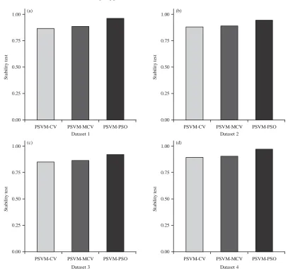
Fig. 2(a-d): Stability test results of the used methods for the four datasets Further, a stability test which is an indicator of
descriptor selection consistency, using the Jaccard index is utilized to highlight the performance of the PSVM-PSO.
Let, D1 and D2 be subsets of the selected descriptors such that D1, D2fD, for a number of solutions D = {D1,…, Dr}, the stability test is defined as:
(17) r 1 r
i 1 J j i 1
i j
I (D , D ) 2
Stability test r(r 1)
where, Ij(Di, Dj) is the Jaccard index which is defined as the size of the intersection between any two groups divided by the size of their union. Mathematically, it is defined as:
1 2
J 1 2
1 2
D D I (D ,D )
D D
The higher the stability test value is, the more stable the descriptor selection is. Figure 2 shows the stability test values on the four datasets for the PSVM-PSO, PSVM-MCV and the PSVM-CV. As can be seen from Fig. 2, the PSVM-PSO displays the high rate of stability compared with PSVM-MCV and PSVM-CV.
CONCLUSION
[image:7.612.101.508.83.466.2]REFERENCES
Algamal, Z.Y. and M.H. Lee, 2015. Penalized logistic regression with the adaptive LASSO for gene selection in high-dimensional cancer classification. Expert Syst. Appl., 42: 9326-9332.
Algamal, Z.Y., M.H. Lee, A.M. Al Fakih and M. Aziz, 2017. High dimensional QSAR classification model for anti hepatitis C virus activity of thiourea derivatives based on the sparse logistic regression model with a bridge penalty. J. Chemom., 31: e2889-e2889.
Al Fakih, A.M., Z.Y. Algamal, M.H. Lee, H.H. Abdallah and H. Maarof et al., 2016. Quantitative structure-activity relationship model for prediction study of corrosion inhibition efficiency using two stage sparse multiple linear regression. J. Chemom., 30: 361-368.
Becker, N., G. Toedt, P. Lichter and A. Benner, 2011. Elastic SCAD as a novel penalization method for SVM classification tasks in high-dimensional data. BMC. Bioinf., 12: 138-151.
Bi, J., K. Bennett, M. Embrechts, C. Breneman and M. Song, 2003. Dimensionality reduction via sparse support vector machines. J. Mach. Learn. Res., 3: 1229-1243.
Bradley, P.S. and O.L. Mangasarian, 1998. Feature selection via concave minimization and support vector machines. Proceedings of the 15th International Conference on Machine Learning (ICML'98) Vol. 98, July 24-27, 1998, ACM, Morgan Kaufmann Publishers Inc., San Francisco, California, USA., ISBN:1-55860-556-8, pp: 82-90.
Broman, K.W. and T.P. Speed, 2002. A model selection approach for the identification of quantitative trait loci in experimental crosses. J. Royal Stat. Soc. Ser. B., 64: 641-656.
Cao, G.P., M. Arooj, S. Thangapandian, C. Park and V. Arulalapperumal et al., 2015. A lazy learning-based QSAR classification study for screening potential histone deacetylase 8 (HDAC8) inhibitors. SAR. QSAR. Environ. Res., 26: 397-420. Cervantes, J., F. Garcia-Lamont, L. Rodriguez, A. Lopez and J.R. Castilla et al., 2017. PSO-based method for SVM classification on skewed data sets. Neurocomput., 228: 187-197.
Chen, J. and Z. Chen, 2008. Extended bayesian information criteria for model selection with large model spaces. Biometrika, 95: 759-771.
Chen, K.H., K.J. Wang, K.M. Wang and M.A. Angelia, 2014. Applying particle swarm optimization-based decision tree classifier for cancer classification on gene expression data. Appl. Soft Comput., 24: 773-780.
Cong, Y., B.K. Li, X.G. Yang, Y. Xue and Y.Z. Chen et al., 2013. Quantitative structure-activity relationship study of influenza virus neuraminidase A/PR/8/34 (H1N1) inhibitors by genetic algorithm feature selection and support vector regression. Chemom. Intell. Lab. Syst., 127: 35-42.
Daszykowski, M., B. Walczak, Q.S. Xu, F. Daeyaert and M.R. de Jonge et al., 2004. Classification and regression trees studies of HIV reverse transcriptase inhibitors. J. Chem. Inf. Comput. Sci., 44: 716-726. Dong, H. and G. Jian, 2015. Parameter selection of a support vector machine, based on a chaotic particle swarm optimization algorithm. Cybern. Inf. Technol., 15: 140-149.
Fan, J. and R. Li, 2001. Variable selection via nonconcave penalized likelihood and its oracle properties. J. Am. Stat. Assoc., 96: 1348-1360. Ikeda, K. and N. Murata, 2005. Geometrical properties of
Nu support vector machines with different norms. Neural Comput., 17: 2508-2529.
Jung, Y. and J. Hu, 2015. AK-fold averaging cross-validation procedure. J. Nonparametric Stat., 27: 167-179.
Kennedy, J. and R. Eberhart, 1995. Particle swarm optimization. Proceedings of the IEEE International Conference on Neural Networks, Volume 4, November 27-December-1, 1995, Perth, WA., pp: 1942-1948.
Khajeh, A., H. Modarress and H. Zeinoddini Meymand, 2012. Application of modified particle swarm optimization as an efficient variable selection strategy in QSAR/QSPR studies. J. Chemom., 26: 598-603.
Kiran, M.S., 2017. Particle swarm optimization with a new update mechanism. Appl. Soft Comput., 60: 670-678.
Lai, C.M., W.C. Yeh and C.Y. Chang, 2016. Gene selection using information gain and improved simplified swarm optimization. Neurocomputing, 218: 331-338.
Li, Y., Y. Kong, M. Zhang, A. Yan and Z. Liu, 2016. Using Support Vector Machine (SVM) for classification of selectivity of H1N1 neuraminidase inhibitors. Mol. Inf., 35: 116-124.
Liang, Y., C. Liu, X.Z. Luan, K.S. Leung and T.M. Chan et al., 2013. Sparse logistic regression with a L1/2 penalty for gene selection in cancer classification. BMC. Bioinf., 14: 1-12.
Lin, S.W., K.C. Ying and S.C. Chen, 2008. Particle swarm optimization for parameter determination and feature selection of support vector machines. Expert Syst. Applic., 35: 1817-1824.
Liu, Y., H.H. Zhang, C. Park and J. Ahn, 2007. Support vector machines with adaptive Lq penalty. Comput.
Liu, Z., S. Lin and M. Tan, 2010. Sparse support vector machines with L_{p} penalty for biomarker identification. IEEE. ACM. Trans. Comput. Biol. Bioinf., 7: 100-107.
Lu, Y., S. Wang, S. Li and C. Zhou, 2011. Particle swarm optimizer for variable weighting in clustering high-dimensional data. Mach. Learn., 82: 43-70. Meijer, R.J. and J.J. Goeman, 2013. Efficient
approximate K fold and leave one out cross validation for ridge regression. Biom. J., 55: 141-155.
Mirjalili, S. and A. Lewis, 2013. S-shaped versus V-shaped transfer functions for binary particle swarm optimization. Swarm Evolut. Comput., 9: 1-14.
Pang, Z., B. Lin and J. Jiang, 2016. Regularisation parameter selection via bootstrapping. Aust. N. Z. J. Stat., 58: 335-356.
Park, H., F. Sakaori and S. Konishi, 2014. Robust sparse regression and tuning parameter selection via the efficient bootstrap information criteria. J. Stat. Comput. Simul., 84: 1596-1607.
Roberts, S. and G. Nowak, 2014. Stabilizing the lasso against cross-validation variability. Comput. Stat. Data Anal., 70: 198-211.
Sabourin, J.A., W. Valdar and A.B. Nobel, 2015. A permutation approach for selecting the penalty parameter in penalized model selection. Biom., 71: 1185-1194.
Shen, Q., W.M. Shi, W. Kong and B.X. Ye, 2007. A combination of modified particle swarm optimization algorithm and support vector machine for gene selection and tumor classification. Talanta, 71: 1679-1683.
Wang, L., J. Zhu and H. Zou, 2008. Hybrid huberized support vector machines for microarray classification and gene selection. Bioinf., 24: 412-419.
Wen, J.H., K.J. Zhong, L.J. Tang, J.H. Jiang and H.L. Wu et al., 2011. Adaptive variable-weighted support vector machine as optimized by particle swarm optimization algorithm with application of QSAR studies. Talanta, 84: 13-18.
Xing, J.J., Y.F. Liu, Y.Q. Li, H. Gong and Y.P. Zhou, 2014. QSAR classification model for diverse series of antimicrobial agents using classification tree configured by modified particle swarm optimization. Chemom. Intell. Lab. Syst., 137: 82-90.
Zhang, H.H., J. Ahn, X. Lin and C. Park, 2005. Gene selection using support vector machines with non-convex penalty. Bioinf., 22: 88-95.