Scarring effects of the first
labour market experience:
A sibling based analysis
The Institute for Labour Market Policy Evaluation (IFAU) is a research insti-tute under the Swedish Ministry of Industry, Employment and Communica-tions, situated in Uppsala. IFAU’s objective is to promote, support and carry out: evaluations of the effects of labour market policies, studies of the function-ing of the labour market and evaluations of the labour market effects of meas-ures within the educational system. Besides research, IFAU also works on: spreading knowledge about the activities of the institute through publications, seminars, courses, workshops and conferences; creating a library of Swedish evaluational studies; influencing the collection of data and making data easily available to researchers all over the country.
IFAU also provides funding for research projects within its areas of interest. There are two fixed dates for applications every year: April 1 and November 1. Since the researchers at IFAU are mainly economists, researchers from other disciplines are encouraged to apply for funding.
IFAU is run by a Director-General. The authority has a traditional board, con-sisting of a chairman, the Director-General and eight other members. The tasks of the board are, among other things, to make decisions about external grants and give its views on the activities at IFAU. A reference group including repre-sentatives for employers and employees as well as the ministries and authori-ties concerned is also connected to the institute.
Postal address: P.O. Box 513, 751 20 Uppsala Visiting address: Kyrkogårdsgatan 6, Uppsala Phone: +46 18 471 70 70
Fax: +46 18 471 70 71 ifau@ifau.uu.se www.ifau.se
Papers published in the Working Paper Series should, according to the IFAU policy, have been discussed at seminars held at IFAU and at least one other academic forum, and have been read by one external and one internal referee. They need not, however, have undergone the standard scrutiny for publication in a scientific journal. The pur-pose of the Working Paper Series is to provide a factual basis for public policy and the public policy discussion.
Scarring effects of the first labour market experience: A sibling based analysis♣
Oskar Nordström Skans* 2004-11-10
Abstract
The paper studies the relationship between teenagers’ first labour market experience and subsequent labour market performance using data on all Swedish youths graduating from vocational high school programmes in 1991– 94. Sibling fixed-effects combined with detailed data on high school pro-grammes, grades and work experience during high school are used in order to identify the causal long-run effects of experiencing unemployment subsequent to graduation. The results show a 3 percentage-points increase in the unem-ployment probability and a 17 % reduction in annual earnings after 5 years due to post-graduation unemployment. The results thus show that teenage labour market failure is in fact costly even though most teenagers have relatively short unemployment spells.
JEL-code: J64
Keywords: Youth unemployment, Scarring, State dependence, Siblings
♣
I thank Olof Åslund, Erika Ekström, Peter Fredriksson, Alan Krueger, Rafael Lalive, Eva Mörk and seminar participants at IFAU, SOFI, The Economic Council of Sweden and the 2004 EEA conference for helpful comments and suggestions.
*
Institute for labour market policy evaluation (IFAU), Email: oskar.nordstrom_skans@ifau.uu.se. Phone +46 18 471 70 79.
Table of contents
1 Introduction ... 3
2 Background... 4
2.1 Previous literature... 4
2.2 The economic environment and institutions... 7
3 The empirical framework ... 10
4 Data and descriptive statistics... 13
4.1 Data... 13
4.1.1 Education and work experience... 13
4.1.2 Demographic variables ... 14
4.1.3 Unemployment and employment... 15
4.1.4 Aggregate covariates ... 16
4.2 Descriptive statistics ... 18
5 Sibling fixed effects estimates ... 21
5.1 Different forms of duration dependence... 26
6 Sub-sample OLS estimates ... 27
7 Concluding remarks... 32
References... 33
Appendix A: Covariates... 37
1 Introduction
Young workers have higher entry rates into unemployment and higher exit rates out-of unemployment than older workers. As a result, young worker have relatively short unemployment spells which may suggest that youth unem-ployment is a harmless state requiring little attention from the policymakers. Nevertheless, most countries provide specific active labour market programs targeted at young workers. One possible rationale for policymakers’ focus on youth unemployment is that some young workers may experience very long-term negative effects even from short unemployment spells, a phenomenon usually referred to as “state dependence” or “scarring”.
There is a vast previous literature on the long-term consequences of unemployment. However, identifying causal effects of past unemployment is a difficult task due to problems with unobserved heterogeneity: the estimated effects will be larger than the true effects if workers differ in their underlying probability of being unemployed for reasons that we are unable to control for. Thus, separating the effects of unobserved heterogeneity from the causal effects of previous unemployment (i e the true scarring effect) is a fundamental problem in this literature. Most previous studies have relied on distributional assumptions regarding the unobservable component in order to solve this problem. The results in these studies suggest that unemployment do indeed have persistent negative effects, at least for prime aged workers. However, the estimates are likely to be biased towards this finding unless the distributional assumptions are fulfilled.
This paper explores a uniquely rich data set containing family identifiers facilitating the use of within-family comparisons as a tool to separate causal effects from unobserved heterogeneity. The identifying assumption is that sibling fixed effects together with individual level covariates capture all relevant heterogeneity. We study the early labour market careers of four entire cohorts of graduates from Swedish vocational high school programmes and use detailed information on grades, field of study and in-school work experience as controls for differences between siblings. The detailed individual level information have a large impact on the variable of interest in models without sibling fixed effects, but only a minor impact once we include sibling fixed effects. This suggests that the within-family-comparisons model is indeed a powerful tool for removing a potential bias stemming from individual
heterogeneity. However, it comes at a cost of a substantial reduction in sample size and degrees of freedom.
The results show that unemployment subsequent to graduation gives rise to significant “scars” that remain for at least 5 years after the initial ployment experience. The magnitude is far from negligible: 50 days of unem-ployment in the year following high school graduation leads to a 3 percentage-points higher probability to experience a similar period of unemployment (and a decrease in total annual earnings of 17 %) 5 years later.
We also estimate models controlling for observable family background instead of using sibling fixed effects. This introduces a bias to the estimates but increases the precision which allows us to study the effects in smaller sub-samples. The results indicate that the long run effects of teenage unemployment are similar across various sub-groups defined by gender, ethnicity or business-cycle at the time of labour market entry which strengthen our belief in the results.
The paper is structured as follows: Section 2 gives the institutional background and Section 3 defines the empirical model. Section 4 describes the data and presents some descriptive statistics. Section 5 shows the sibling fixed effects estimates and Section 6 show sub-sample estimates. Section 7 concludes.
2 Background
2.1 Previous literature
Unemployment may have negative effects on future labour market performance for several different reasons: A first explanation has to do with human capital, either due to the forgone work experience during the unemployment spell or, perhaps more seriously, if people’s skills actually deteriorate during a spell of inactivity as suggested by Edin & Gustavsson (2004). It is thus possible that (the market value of) skills acquired during high school may depreciate relatively fast unless the skills are used.
Second, if hiring takes place under uncertainty about worker productivity, employers may use previous unemployment spells as a screening device in
their hiring process and thus prefer to hire workers with shorter unemployment histories.1
Third, institutions such as seniority rules that protect workers with long tenure on the expense of short tenured workers will give those receiving jobs early an advantage over those receiving their jobs later. This advantage may be important whenever a firm is hit by negative a shock, even if the shock arrives much later (see e g Eliasson & Storrie, 2004).
Finally, very young workers’ preferences for work and leisure may be influenced by their early experiences. Some support in this direction can be found in the literature on social interactions (for example Hedström, Kolm & Åberg, 2003, and Stutzer & Lalive, 2003) which argue that the stigma of unemployment is affected by the labour market position of the reference group and that a smaller stigma may lower the outflow from unemployment. If unemployment per se causes teenagers to spend more time with other unemployed people, they may eventually have a reference group with weaker labour force attachment. According to the above logic, this could reduce the stigma of unemployment and thus also the incentive to work.
The empirical literature on scarring or “state-dependence” dates back to the early 1980s with papers by Ellwood (1982), Corcoran (1982) and Heckman &
Borjas (1980). The papers by Ellwood and Heckman & Borjas clearly
identified the empirical obstacles that must be overcome in order to identify causal (or “true”) state dependence. The basic problem is to separate causal effects from unobserved heterogeneity since any unobserved characteristics that causes a person to be unemployed at one point in time is likely to do so also in the future. There are basically three solutions that have been applied in the empirical literature: i) rely on observable characteristics ii) use aggregate unemployment as an instrumental variable or iii) make distributional assump-tions regarding the unobserved component.
Ellwood (1982) studies US data from the NLSY and concludes that the effect of early non-employment on future employment probability is small but that the effect on wages is large. Corcoran (1982) studies a NLS sample of women and reaches similar conclusions regarding wages but also finds
1
In a survey of Swedish firms by Agell & Bennmarker (2002), employers confirm this idea. Further support is found in Eriksson and Lagerström (2004) who show that unemployed job seekers receive fewer job contacts than employed job seekers even after controlling for all information available to the employers using data from a Swedish “applicant data base”.
evidence of persistent negative employment effects. Heckman & Borjas (1980), in their empirical application, find little evidence of true state dependence. The most recent study on US data is by Mroz & Savage (2001) that use data from the NLSY in a dynamic model with lagged instruments and find significant effects four years after an unemployment spell on both annual earnings (approximately 1 % from 10 weeks of unemployment) and the unemployment probability (4 % from 10 weeks of unemployment). Evidence suggesting that unemployment may affect future wages through “implicit contracts” can be found in the paper by Beadry & DiNardo (1991) who show that wages are affected by the aggregate unemployment rate at the time of hiring.
For the UK Arulampalam, Booth & Taylor (2000) used data from the British Houshold Panel Survey (BHPS) and a random effects specification finding evidence of state dependence in unemployment, a result confirmed by Arulampalam (2002) using a similar identification strategy. In addition she finds that the effects were smaller for workers under 25. Studies on British data that rely on observables for identification include Arulampalam (2001) that finds a 14 % earnings loss 3 years after an unemployment spell in the BHPS, Gregory & Jukes (2001) that uses administrative data and find a short-run effect of unemployment incidence and a long run effect of unemployment duration and Gregg (2001) using the National Child Development Survey who finds evidence of state dependence in unemployment, particularly for men. Gregg (2001) also uses aggregate unemployment as an instrument for individual unemployment which, surprisingly, generates larger estimates. Burgess, Propper, Rees & Shearer (2003) use a different approach and controls for aggregate unemployment and find negative effects for the non-skilled of entering the labour market in a cohort with high youth unemployment.
Evidence from other countries are scarce, Hämäläinen (2003) applies a cor-related random effects model to Finnish data and finds evidence of short-term scarring effects, in particular for low-educated workers. Knights, Harris and Loundes (2002) use a similar method on Australian data finding evidence of scarring effects of unemployment. Muhleisen & Zimmerman (1994) applies a random effects probit to German data and find evidence of short run state dependence. Clark, Gorgellis & Sanfey (1999) also use German data and show that unemployment leads to long-lasting disutility effects, at least for men.
There is also a potentially relevant literature on plant closings. The surveys in Kletzer (1998) and Fallick (1996) provide evidence of negative effects from plant closings during at least a few years. A recent example on Swedish data is
Eliasson & Storrie (2004) how show that there are significant negative effects of plant closings that can be reinforced when the business cycle turns bad, even several years after the initial shutdown. However, it is not evident to which extent evidence from plant closings can be generalised to other sources of unemployment.
Little other relevant evidence exists on Swedish data. Exceptions are Åslund & Rooth (2003) who find that refugee immigrants that where placed in munic-ipalities with high unemployment rates performed worse at the labour market for a long period of time and Hansen & Lofstrom (2003) who study the dynamics of welfare receipt among immigrants and native Swedes.
Overall, the evidence suggests that scarring is a real phenomenon.2 On the other hand, the results suggest that the effects are smaller for young workers and, furthermore, estimates of scarring effects are likely to be upward biased if the observed covariates or distributional assumptions fail to appropriately control for individual heterogeneity.
2.2 The economic environment and institutions
The analysis of this paper is based on data on the cohorts graduating from Swedish high schools between 1991 and 1994. The cohorts are followed until the year 2001. This is the most turbulent period in the Swedish labour market since World War II: The unemployment rate which had been below 5 % since the 1960s (and was below 2 % in the late 1980s) suddenly increased to 8 % in the early 1990s. Explanations for this severe recession are typically based on a combination of bad policies and bad luck (see e g Holmlund 2003). The unemployment rate remained high until the late 1990s when it started to decline and by the year 2002 the unemployment rate had declined to 4 %. The time pattern for youth unemployment showed a similar time pattern to the overall unemployment rate (see Figure 1).
2
The main exceptions are the early papers by Ellwood (1982), for employment, and Heckman & Borjas (1980). However it should be noted that these papers, as pointed out in the papers themselves, use very small (N = 364 and 122) and non-representative samples, which suggests that not too much weight should be put on these empirical results.
0 .0 5 .1 .1 5 .2 U n em pl oy m e n t r a te 1986 1988 1990 1992 1994 1996 1998 2000 2002 Year
Unemployment rate Unemployment rate, age 16-24
Source: The Swedish Labour Force Surv ey s (AKU), SCB.
Figure 1: Unemployment rates 1986–2002.
The 1990s also saw a rapid expansion of the proportion of the working aged population enrolled in some form of education. Part of this expansion was due to increased participation in regular education but another reason was active policy measures aimed at the unemployed (and to some extent also to the employed) such as the “Adult education initiative”. As a result, the employ-ment to population rates did not recovered as well as the unemployemploy-ment rates after the recession, especially not for younger workers (see Figure 2).
Our empirical model will account for the varying business cycle environ-ment through year dummies. Furthermore, in a robustness analysis we will estimate separate effects separately for the cohort that graduated in 1991 when labour market conditions still were relatively decent in order to see how the estimated effects vary with the business cycle.
.3 .4 .5 .6 .7 .8 E m p loy m en t t o p oul at io n rat e 1986 1988 1990 1992 1994 1996 1998 2000 2002 Year
Employment rate, 16-64 Employment rate, 16-24
Source: The Swedish Labour Force Surv ey s (AKU), SCB.
Figure 2: Employment to population rates 1986-2002.
The Swedish educational system requires that all children start school during their 7th year and attend 9 years of compulsory schooling. After finishing 9th grade (during their 16th year) most students choose to start high school. As an example, 85 % of those born 1973 graduated from high school before the age of 20 (see Table 1 below).
High school students are enrolled in one of several possible “programmes”. Admissions to the programmes are based on the compulsory school grade point average (GPA) whenever there are more applicants than can be admitted.
During the period of study (1991−94) the programmes were standardized into
three main categories: academic 3-year programmes, academic 2-year pro-grammes and vocational 2-year propro-grammes.
As is evident from Table 1, most university students came from the 3-year programmes while employment at age 20 was much higher amongst the graduates from 2-year programmes. On some locations there was also a
piloting scheme with vocational 3-year programmes.3 Since the role of these
3
Due to a reform of the vocational programmes in the early 1990s, all Swedish high school students graduating after 1994 received a 3 year long education that qualifies for university studies. However, this institutional change does not apply to the cohorts included in this study.
programmes mainly was as substitutes for the shorter vocational programmes, they will be treated as identical to the shorter programmes in the analysis (see Ekström, 2002, for an evaluation of the pilot-programmes).
Table 1: The high school programmes
Education at age 20 Ni Share of total (Ni/N) Employed at age 20 Tertiary education at age 27
Less than high school 16,234 0.15 0.33 0.08
2-year high school 36,898 0.34 0.46 0.15
3-year high school 46,247 0.43 0.33 0.53
Tertiary education 9,300 0.09 0.17 1
All 108,679 1 0.36 0.37
Note: Groups are defined from completed high school programmes. Sample includes all individuals born in 1973 that lived in Sweden in both 1993 and 2000 (excluding 2000 missing values). Employment is for November. “Tertiary education” includes graduates of the 4-year high school engineering programme.
In theory all students from the academic programmes (but, in general not those from vocational programmes) where eligible for university admission. However, in practice most university programmes had requirements that ex-cluded applicants from the 2-year academic programmes. As a consequence, the transition rates from the 2-year academic programmes were as low as from the vocational programmes. It should be noted, however, that the adult edu-cation system (Komvux) provided an opportunity to complement the studies for those that wished to qualify for university after graduating from the 2-year programmes.
3 The
empirical
framework
Based on Gregg (2001) we may identify three possible reasons for an association between teenage unemployment and future labour market per-formance:
1. Individual heterogeneity: some people are more prone to unemploy-ment due to preferences or innate ability.
2. Labour market persistence: a young worker may become unemployed due to poor labour market conditions. The individual
will be more likely to be unemployed in the future as well, if these conditions are persistent.
3. Scarring: Unemployment in itself may generate unemployment in the future either through firm discrimination, human capital depre-ciation or other mechanisms.
More formally we can assume a two-period data generating model: in period 0 the worker enters the labour market and in period t we measure the effects of unemployment in period 0. Let X be a vector of observed individual i
specific characteristics, and let R denote an unobserved individual specific i
effect for individual i having the effect νt at time t. LetA be the labour market itj
conditions faced by the individual at time t at the labour market j. Allowing for unemployment scarring in period t we get a model determining the
unemployment of individual i in period 0 (denoted by U ) and the labour i0
market performance in period t (denoted by Yit):
io i j io i io X A R U =
β
0 +λ
0 + +ε
(1) it i t io t j it t t i it X A U vR Y =β
+λ
+γ
+ +ε
. (2)In the empirical applications of this equation t will range from 1 to 10 (at most). Our main identifying strategy uses sibling fixed effects (αiS) to proxy for
the individual specific effect vtRi and estimate the equation:4 it S it io t j it t t i it X A U u Y =
β
+λ
+γ
+α
+ . (3)Thus, the identifying assumption behind the sibling fixed effects estimates is that all differences between siblings that are correlated with both
4 One common method used in order to identify state dependence is to rely on distributional
assumptions such as correlated random effects models. However, one drawback with this method is that the underlying assumptions are difficult to validate. Furthermore, since we specifically look at the effect of the initial state we only have one observation per individual in each regression, making it impossible to include individual-specific random effects.
ployment at time 0 and labour market performance at time t are captured by the individual specific variables included in X, i.e. such that
cov (uit , Ui0) = 0 for all t.
We also estimate an “OLS-specification” where we proxy the unobserved individual component by observable family characteristics (Zit) instead of the
sibling fixed effect:
it it t io j it t t i it
X
A
U
Z
Y
=
β
+
λ
+
γ
+
φ
+
η
. (4)This model can only be given causal interpretation if it can be argued that all
differences between individuals that are correlated with both initial
unemploy-ment and subsequent performance are captured either by the observed indi-vidual specific information (the X-vector) or the observed family background variables (the Z-vector) , i.e. such that cov (ηit , Ui0) = 0 for all t. The main
reason for estimating the OLS specification is that it greatly increases the sample size and thus the precision in the estimates. Since the identifying assumptions are stronger in the OLS specification, we will only use it to check for differences in estimates between different sub-samples.
The aim of the applied empirical models is to generate a situation where we are comparing two groups that are (conditionally) identical, where one group did become unemployed, and the other did not, and compare the subsequent outcomes of these two groups. The logic behind the models rest on the standard assumption (see e g Pissarides 2000) that matching frictions are important at the labour market (see Ridder & van den Berg, 2003, for empirical evidence). Matching frictions imply that even identical individuals will end up in different states when first entering the labour market due to factors that can be treated as purely random. Thus, it should be possible to identify scarring effects by conditioning on individual characteristics, given sufficiently good data.5
5
The use of sibling data in the literature on returns to education has been criticised by e.g. Griliches (1979) and Bound & Solon (1999) on concern that if indeed siblings are so alike, why do they end up with different education? In the current application the corresponding question would be “why do they end up in different initial states?” The answer is “due to matching frictions”.
4
Data and descriptive statistics
The data used in this paper cover four entire cohorts of young individuals graduating from vocational and 2-year academic high school programmes between 1991 and 1994. The exclusion of 3-year academic programmes is motivated by a wish to minimise the impact of direct transitions into further education and the assumption that graduates from the 2-year programmes in general are aiming at employment (rather than further education) after gradu-ation. The only other restriction put on the (base) sample is that the graduates should be aged 18 or 19 at graduation.
4.1 Data
The general source of data is the IFAU database that combines data from various registers from Statistics Sweden and the National Labour Market Board. The original data sources are the high school examination registers (UREG) which contain information on grades and courses for all high school graduates, a longitudinal income register (LOUISE) that links family members to each other and contain information on demographics and socioeconomic factors, the employment register (RAMS) containing information on employ-ment and earnings and an unemployemploy-ment register (HÄNDEL) which contain information on spells of registered unemployment at public employment services.
4.1.1 Education and work experience
The individuals included in this study are all graduates aged 18 or 19 by the end of the graduation year from i) vocational 2-year programmes ii) theoretical 2-year programmes and iii) the vocational 3-year pilot programmes.
Each student takes a set of courses, some of which are compulsory for all
students in the programme, and some of which are chosen by the student.6 Our
data includes detailed information on course specific grades from which we construct three different variables: Overall grade point average (GPA), field
6
The selection of courses taken by each student is a complicated process: Many programmes have different specific fields to which the students have to apply in advance, e.g. electricians can be either general electricians or specialised on telecommunication. In addition, some courses are chosen by the student; typically this choice is between a predetermined set of courses which may vary between schools.
specific grade point average (FGPA) capturing the average grade in courses that are directly related to the field of the programme (e.g. “Construction” for
the Construction workers programme)7 and a dummy for students that either
failed or received the grade 1 (out of 5) in any course (Failed).
By nature, high school graduates have very little labour market experience. However, we use information on labour earnings during the final complete calendar year in high school and a dummy for whether the student was employed in November during the same year. The idea is that these variables should capture both unobserved ability (e g in the form of motivation) and potential effects of in-school work experience (see e g Häkkinen, 2004).
4.1.2 Demographic variables
A key set of background information refers to the parents of the graduates. In constructing these data, step-parents and biological parents are treated equally since the data are based on household information. These data are used both to construct sibling-pairs and in order to generate family characteristics for the OLS specification.
The sibling fixed-effect is of course a key variable. It is identified from the identity of the (household) mother. Restricting the analysis to children with identical father and mother reduces the sample somewhat primarily through the exclusion of graduates from single-mother households but does not affect the estimates significantly.
The observable characterises of the parents used in the OLS specification captures: Immigration status, Education, Employment, Earnings,
Self-employment, Taxed capital income, Disposable income and Welfare assistance.
In addition, the regressions without sibling fixed effects also include parish of
residence dummies in order to further capture the socio-economic background
of the graduates. A parish is a part of a municipality and the sample includes
7
The FGPA is constructed from the data by looking at the courses most often taken by graduates of each programme, excluding general courses such as Swedish and mathematics. The FGPA-variable is the average grade within the specific courses taken by each student. The ordinary GPA is used for the (few) students that did not take any field specific courses and for all students from the 3-year vocational programmes in the piloting scheme since their field specific grades are missing in the data. In order to assess the robustness of our results we also estimate a model including only (18-year old graduates of ) the 2-year vocational programmes.
observations from 2048 parishes. All variables are measured during the graduates last year in high school.8
Individual-level demographic variables capture year of birth, gender and
country of birth (Swedish, other Nordic county or the rest of the world). The
only individual-level control variable dated after the graduation year is a dummy for military service. The Swedish military is based on conscription, and as a result, a large fraction of the males (and very few female volunteers) enter the military at some point in time. The decision on if, when and how the worker will fulfil his service is usually taken at age 17. The decision can be changed (in particular the timing) for different reasons. However, for the purpose of this study it is considered to be an exogenous event. Since the results for men and women are very similar in our robustness check, this should not be a major concern.
4.1.3 Unemployment and employment
One of the two alternative variables used in order to measure initial labour market status is a dummy for whether the graduate became unemployed during the year following graduation. The unemployment data captures the number of
days a worker is registered as unemployed at the public employment service,9
and a dummy is given the value one if a worker is registered as unemployed for
at least 50 days between September and May, and zero otherwise.10
Unemploy-ment in the subsequent years are measured using corresponding definitions. The choice of September to May for the measure of unemployment is based on the assumption that registered unemployment experiences during the summer months are less informative than the rest of year for young workers. Qualitatively, the results are completely robust to changes in the somewhat arbitrary cut-off at 50 days in order to be classified as unemployed.
The alternative explanatory variable is employment after graduation. Em-ployment is measured using Statistics Sweden’s earnings-based definition which codes workers with earnings corresponding to 4 hours of work in November as employed. The same definition is also used when employment is considered as an outcome variable during the subsequent years.
8
The exception being data on taxed capital income that is taken from the graduation year since data for 1990 where unavailable.
9
We do not include time spent in active labour market programmes. Qualitatively, the results are very similar if time spent in labour market programmes is treated as unemployment.
In addition to studying the effects on employment and unemployment, we will also study the effects on the natural logarithm of annual labour earnings. In the base-line specification observations without earnings are changed to the minimum amount in the data (100 SEK ≈ €10) but we also estimate a model conditional on being employed in November, which excludes the zero earnings cases. Labour earnings are measured by calendar-year so the analysis of the effects of initial unemployment on earnings will start two years after graduation since the first year overlaps with the initial unemployment period (see above). Figure 3 shows the time axis for the analysis.
4.1.4 Aggregate covariates
Aggregate unemployment rates are calculated using the unemployment register matched with a population-wide register of education. A programme-specific unemployment-to-population rate (henceforth referred to as “unemployment rate”) is calculated for each combination of programme, municipality and year
using the 50 days May to September procedure explained above.11 The
calculation is based on individuals aged 21 to 35 during the graduation year (i e they are 3 to 16 years older than the graduates) in order to get a measure of the labour market conditions relevant for relatively young workers. An overall municipality unemployment rate is also calculated for each year using the same procedure and population but without separating the different programmes. Furthermore, all regressions include dummies for graduation year (interacted with birth year) in order to remove all aggregate business cycle effects.
11
Unique programme unemployment rates can not be calculated for the 3-year vocational programmes in the piloting scheme since there are no older graduates. The 2-year programmes with corresponding occupations are used instead (see Ekström, 2002, for the correspondences).
Calendar year Academic year
Initial unemployment is measured (t = 0), September through May
Unemployment at t = 1 September through May
Unemployment at t = 2 September through May Earnings at t = 1
Employment at t = 1
June, graduation from high school
Earnings at t = 2
Employment at t = 2
November, initial employment is measured (t = 0)
Figure 3: The time axis.
Calendar year Academic year
1st year in high school September to early June
2nd year in high school September to early June In-school earnings and
parental information In-school November employment June, graduation from 9th grade January June, graduation from high school
4.2 Descriptive statistics
Table 2 shows data on unemployment and employment during the year
following graduation. When reading the table it should be noted that the different states are not mutually exclusive, i.e. it is possible for the same individual to be recorded in more than one of the states.
Table 2: Initial labour market status
Unemployed Graduation
year At least 1 day >49 days Employed N
1991 0.47 0.21 0.62 45,348
1992 0.50 0.29 0.35 46,796
1993 0.41 0.23 0.26 44,443
1994 0.35 0.19 0.33 34,659
All 0.44 0.23 0.39 171,246
Note: States are not mutually exclusive. “Unemployed” implies registered as openly unemployed (thus excluding e.g. participation in labour market programmes) between September of graduation year and May of the following year. Employment is for November of graduation year.
The table shows a surprising time-pattern for the unemployment rates that are falling between 1991 and 1994. This is quite in contrast to the evolution of the macro environment described in Figure 1. One explanation for this apparent anomaly is an increase in the fraction pursuing further education. During the period there was a gradual increase in the fraction of students acquiring one additional year of education directly after graduating from the 2-year vocational programmes, probably due to a combination of worsening labour market conditions and the introduction of 3-year vocational pro-grammes. In order to assess the importance of further education, the paper will use both employment and unemployment as indicators of initial labour market performance and use several different sample restrictions when estimating the OLS sample (see Section 5).
0 .2 .4 .6 F ra c ti on u n e m pl oy e d 1 2 3 4 5 6 7 8 9
Years after graduation
If unemployed at t=0 If not unemployed at t=0 Unemployment (50 days)
Figure 3: Unemployment probabilities depending on post-graduation (t = 0)
unemployment.
Table A1 in Appendix A shows descriptive statistics for the main time
invariant covariates used in the analysis. Figure 3 and Figure 4 show the development over time for unemployment and employment separated by initial labour market performance. It is clear that those unemployed after graduation are unemployed during the following ten years to a much higher degree. It is equally true that those employed after graduation have a higher probability of being employed during the 9 years following graduation.
Figure 5 shows the distribution of the lengths of all unemployment spells
starting during September through May after graduation (thus the same individual may be responsible for several spells). It is evident from the figure that most spells are relatively short; in fact, very few spells are longer than 2 years.12
12
It should be noted that unemployment spells may be broken by participation in active labour market programmes. However, 90 percent of spells are shorter than 2 years even when all reasons for registration at the public employment services (such as e g time in labour market programmes and registration for “on-the-job search”) are included.
Figure 4: Employment probabilities depending on post-graduation (t = 0) employment. 0 .0 0 5 .0 1 .0 15 De ns it y Median 90th percentile 0 100 200 300 400 500 Duration of unemployment
Note: Unemployment spells starting during September through May after graduation. Interuptions < 8 days are disregarded.
Censored at 500 days of uninterupted unemployment (0.3 % of spells).
Figure 5: Duration of unemployment: spells starting the year after graduation.
.2 .4 .6 .8 F rac ti o n em p lo y ed 1 2 3 4 5 6 7 8 9
Years after graduation
If employed at t=0 If not employed at t=0 Employment (November)
5
Sibling fixed effects estimates
The pattern displayed by the descriptive statistics clearly shows a positive correlation between unemployment after graduation and subsequent unemploy-ment. The purpose of this section is to identify causal effects of unemployment subsequent to graduation. The identification strategy uses sibling fixed effects to remove all unobserved heterogeneity that is common within a family. The identifying assumption required is that all relevant differences between siblings are captured by the individual level variables. These variables are Military
Service (dummy), Gender, Age at graduation (18 or 19, interacted with
graduation year), Oldest sibling (dummy), Programme, GPA and Field GPA interacted with programme, Failed (dummy), in-school employment (dummy) and the log of In-school earnings. Note also that included siblings are quite similar in age (at most 4 years in between the siblings) as well as educational choice and performance (only graduates from vocational or shorter high school programs are included).
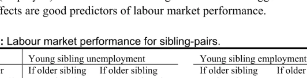
Table 3 shows the raw relationship between the unemployment probabilities
of the youngest and the oldest of each sibling pair. The table shows that workers with siblings that were unemployed (employed) at a certain time after graduation have 5-10 percentage points higher probability of being unem-ployed (emunem-ployed) at the same time after graduation. This suggests that sibling fixed effects are good predictors of labour market performance.
Table 3: Labour market performance for sibling-pairs.
Young sibling unemployment Young sibling employment
Time after graduation (t) If older sibling unemployed If older sibling not unemployed If older sibling employed If older sibling not employed. t = 0 0.30 0.20 0.45 0.38 t = 1 0.40 0.32 0.57 0.46 t = 3 0.35 0.26 0.69 0.54 t = 5 0.21 0.16 0.76 0.66 Note: The table shows the unemployment (employment) probability of younger siblings depending on whether the older sibling was unemployed (employed) at the same time after graduation. The “oldest” sibling is randomly chosen if the birth year is the same for both siblings.
It should be noted that the logic behind the identification strategy rests on the standard (theoretical) assumption that labour markets are characterised by search frictions. Thus, it is likely that even identical individuals receive
different outcomes for reasons that are entirely random. The question posed in this section is whether this randomness has any persistent effects.
Including sibling fixed-effects implies that all individuals without siblings in the base sample are removed. Table A1 in Appendix A shows that this sample is very similar to the overall sample in most characteristics and
Section 5 below shows that this reduced sample produces similar results as the
overall sample when relying on observed characteristics for identification. This should ensure that the results we find are not specific to the sibling sample.
In addition to the individual level variables, the estimated linear probability model also includes two measures of the contemporary labour market con-ditions in the original municipality.13 The first is average unemployment among 15 proceeding cohorts of the same high-school programmes for each year and municipality. The second measure is municipality-year average defined over the same population. Table A2 in Appendix A shows estimates for the control variables during some of the outcome years.
Table 4 shows the estimates of the effects of initial unemployment on future
labour market performance. Estimates are only calculated for the 7 years (6 when the outcome is other than unemployment) for which there are 4 full cohorts since the number of sibling pairs drops dramatically if only one cohort is excluded. The effect of post-graduation unemployment is statistically sig-nificant for all outcome variables during 5 years after graduation: unemploy-ment is increased by 3 percentage-points and employunemploy-ment is decreased by almost 5 percentage points. Annual earnings are reduced by 17 % after 5 years.
13
The reason for conditioning on the original municipality is to avoid controlling for endogenous migration patterns since initial unemployment may affect future mobility.
Table 4: The effects of initial unemployment on labour market performance, sibling fixed effects estimates
Year after graduation (t)
Outcome t = 1 t = 2 t = 3 t = 4 t = 5 t = 6 t = 7 0.074** 0.058** 0.037** 0.038** 0.031** 0.014 0.015 Unemployment (1/0) (0.013) (0.013) (0.012) (0.011) (0.011) (0.009) (0.009) 11.275** 10.331** 4.544** 4.626** 4.299** 2.085 2.139 Days of Unemployment (1.743) (1.829) (1.715) (1.476) (1.374) (1.200) (1.227) -0.027* -0.056** -0.041** -0.036** -0.047** -0.004 -- Employment (1/0) (0.013) (0.013) (0.012) (0.012) (0.012) (0.011) -- -0.320** -0.288** -0.245** -0.175** -0.089 -- ln(Earnings) (0.060) (0.061) (0.061) (0.058) (0.058) Number of cohorts 4 4 4 4 4 4 4 N 17978 17890 17817 17707 17611 17526 17443
Note: Sample includes all graduates observed with a sibling in the sample. Linear probability estimates of the effect of unemployment subsequent to graduation. Regressions include controls for education (Programme, Failed, GPA (by programme), Field GPA (by programme)), Gender, In-school work (log earnings and working in November), Military service (after graduation and at time t), programme specific municipality unemployment at time t, municipality unemployment at time t as well as cohort-birth year interaction dummies. Standard errors are in parentheses. *Significant at 5 % level. **Significant at 1 % level.
Table 5: The effects of initial employment on labour market performance, sibling fixed effects estimates
Year after graduation (t)
Outcome t = 1 t = 2 t = 3 t = 4 t = 5 t = 6 t = 7 0.249** 0.119** 0.074** 0.034** 0.020 0.039** -- Employment (1/0) (0.011) (0.012) (0.011) (0.011) (0.010) (0.010) 1.354** 0.587** 0.289** 0.223** 0.121* 0.185** -- ln(Earnings) (0.045) (0.051) (0.051) (0.052) (0.051) (0.051) -0.062** -0.025* -0.025* -0.016 -0.006 -0.016* -0.012 Unemployment (1/0) (0.012) (0.012) (0.011) (0.010) (0.009) (0.008) (0.007) -5.166** -2.698 -2.018 -1.551 -1.087 -2.238* -2.999** Days of Unemployment (1.486) (1.606) (1.458) (1.292) (1.181) (1.012) (1.038) Number of cohorts 4 4 4 4 4 4 4 N 17978 17890 17817 17707 17611 17526 17443
Note: Sample includes all graduates observed with a sibling in the sample. Linear probability estimates of the effect of unemployment subsequent to graduation. Regressions include controls for education (Programme, Failed, GPA (by programme), Field GPA (by programme)), Gender, In-school work (log earnings and working in November), Military service (after graduation and at time t), programme specific municipality unemployment at time t, municipality unemployment at time t as well as cohort-birth year interaction dummies. Standard errors are in parentheses. *Significant at 5 % level. **Significant at 1 % level.
Using employment as the variable measuring initial labour market performance gives almost as clear a picture. The results presented in Table 5 show that initial employment is associated with higher employment and higher earnings during the entire follow up period of 6 years. The point-estimates when studying the effects of post-graduation employment on future unemploy-ment show a similar pattern, even though some of the estimates are insig-nificant.
The identifying assumption behind the causal interpretation of the estimates is that all relevant differences between siblings are captured by the individual level covariates. In order to get some indication of the importance of heterogeneity within a sibling pair, Figure 7 shows estimates of models with and without the individual level covariates and with and without sibling fixed effects (using the sibling sample and no family background variables in all cases). The results show that the individual level covariates make a large dif-ference without the fixed effects but only a small difdif-ference when the sibling fixed effects are included. This is at least an indication that heterogeneity within siblings pairs is of minor importance in general.
0 .0 3 .0 6 .0 9 .1 2 .1 5 P er c ent age-po int es ti m at es 1 2 3 4 5 6 7
Years after graduation (t)
FE:s & X:s No FE:s, X:s
FE:s, no X:s No FE:s & no X:s
Note: All models include municipality unemploy ment and y ear dummies.
Family characteristics not included in X. All estimates are signif icant except 'FE:s & X:s', t>5
Estimated effects of initial unemployment on subsequent unemployment
Figure 6: Estimates with and without observed individual characteristics (X)
One potential alternative to the sibling fixed effects is to use aggregate unemployment as an instrument for individual unemployment experiences as proposed by Ellwood (1982) and implemented by Gregg (2001). As long as aggregate unemployment rates are uncorrelated with unobserved individual characteristics, it appears to be a valid instrument. However, experiments with this strategy gave two results: First, the standard errors are too large for the analysis to be informative. Second, the IV-estimates are much larger than the corresponding OLS-estimates. This is in line with the results in Gregg (2001) but seems counterintuitive since the point of the instrument is to remove the
upward bias from unobserved heterogeneity. The reason appear to be that high
(municipal) unemployment rates not only increases the unemployment pro-bability of the graduates, but also reduces labour force participation suggesting that the negative effect of poor aggregate conditions is larger than estimated by a first stage regression. Thus, the direct negative effect of poor labour market conditions will be underestimated and the IV estimates of future consequences of an unemployment spell will be exaggerated.
5.1 Different forms of duration dependence
The seminal paper by Heckman & Borjas (1980) defines four different categories of true state dependence: “Markovian dependence” (it takes some time to leave any state), “duration dependence” (exit rates may be declining with time spent in a state), “occurence dependence” (the number of previous spells may matter in the future), and “lagged duration dependence” (the lengths of previous spells may matter in the future).
While it is difficult to separate the different forms of duration dependence from each other, some tentative conclusions can be drawn. First of all, given the short spell lengths displayed in Figure 5 it seems obvious that the long lasting effects are driven by effects after the interruption of the initial spell. Thus, Markovian or (pure) duration dependence can not be the complete story. Furthermore, Table 6 shows estimates where we separate the effects of occurrence and duration of the initial unemployment experience. The results suggest that both lagged occurrence and duration are important in the short run, however, with a “declining marginal effect” of another day of initial unemployment. In the longer run, however, it appears as if the effects of short spells disappears, suggesting that lagged duration dependence is driving the results in the longer perspective. Some caution is warranted though since the
estimates are quite imprecise and few of the differences between estimates are significant.
Table 6: Effects of the amounts of initial unemployment.
Effect on unemployment at year t
Days of initial
un-employment (t = 0) t = 1 t = 3 t = 5 Fraction of total 0.050** 0.024 -0.015 1-20 days (0.018) (0.017) (0.014) 8.7 % 0.067** 0.026 0.013 21-50 days (0.017) (0.015) (0.013) 12.1 % 0.092** 0.051** 0.035** 51-100 days (0.016) (0.015) (0.013) 13.6 % 0.102** 0.041* 0.033* >100 days (0.020) (0.019) (0.017) 8.3 %
Note: Sample includes all graduates observed with a sibling in the sample. Linear probability estimates of the effects of unemployment subsequent to graduation on the probability of being unemployed at least 50 days t years later with separate effects depending on the number of days of initial unemployment. Regressions include sibling fixed effects and controls for education (Programme, Failed, GPA (by programme), Field GPA (by programme)), Gender, In-school work (log earnings and working in November), Military service (after graduation and at time t), programme specific municipality unemployment at time t, municipality unemployment at time t as well as cohort-birth year interaction dummies. Standard errors are in parentheses. *Significant at 5 % level. **Significant at 1 % level.
6
Sub-sample OLS estimates
Even the most conservative interpretation of the sibling fixed effects estimates imply large and significant effects five years after graduation and there are some indications of even more long lasting causal effects. The purpose of this section is to study the robustness of the results to different sample restrictions and to study potential heterogeneity in the scarring effects.
Using a sibling fixed effects specification comes with a substantial cost in degrees of freedom: only 10 percent of the sample is used and the average number of individuals per fixed effect is 2.03. Thus, when studying the effects in smaller sub-samples we would rapidly encounter problems with too large standard errors (as an example, restricting the analysis by gender will reduce the sample by three quarters since all mixed sibling pairs would be dropped). Instead we use an OLS specification where a rich set of observed
socioeconomic family background variables act as a substitute for the sibling fixed effects.
The estimated equations use all available observable family background information (see Section 3.1.2 and Appendix A) instead of the sibling fixed effects. The estimated linear probability model thus includes variables captur-ing ethnicity, education, employment, self-employment, earncaptur-ings, welfare receipts, disposable income and capital income of the parents and geographical location dummies at the parish (sub-municipal) level as well as the individual background characteristics and the two measures of labour market conditions included in the sibling fixed effects specification.
0 .0 3 .0 6 .0 9 .1 2 .1 5 P er c ent age-po int es ti m at es 1 2 3 4 5 6 7
Years after graduation (t)
Sibling FE estimates Upper bound (95 % c i)
OLS estimates (sibling sample) Low er bound (95 % c i)
Note: Conf idence interv alls are f or the sibling FE estimates. The OLS model includes observ able f amily characteristics.
Estimated effects of initial unemployment on subsequent unemployment
Figure 7: A comparison between Sibling Fixed Effects (FE) estimates and OLS
estimates: State dependence in unemployment.
In order to highlight the differences in estimates, Figure 7 and Figure 8 display how the estimates change when we base the identification on observ-ables rather than the sibling fixed effects. Note that the OLS estimates in the figure are based on the siblings-sample in order to isolate the difference in estimates between specifications. The OLS estimates are somewhat larger in magnitude than the sibling fixed effects estimates; the differences are in the
order of one to two standard errors from the sibling model. The confidence intervals of the OLS estimates (not included in the figure) are much smaller since removing the fixed-effects in practice increases the degrees of freedom by a factor of almost 2.
The fact that the OLS specifications generate somewhat larger estimates than the sibling fixed effects specification probably implies that the OLS estimates are upward biased. However, under the implicit assumption that this bias is similar in different sub-samples, we find it worthwhile to use the OLS specification to gain the precision we need for sub-sample analyses to be informative. The idea is that differences between estimates from different sub-samples should be informative even if the estimates themselves are biased.
0 .0 4 .0 8 .1 2 .1 6 .2 .2 4 P er c ent age-po int es ti m at es 1 2 3 4 5 6
Years after graduation (t)
Sibling FE estimates Upper bound (95 % c i)
OLS estimates (sibling sample) Low er bound (95 % c i)
Note: Conf idence interv alls are f or the sibling FE estimates. The OLS model includes observ able f amily characteristics.
Estimated effects of initial employment on subsequent employment
Figure 8: A comparison between Sibling Fixed Effects (FE) estimates and OLS
estimates: State dependence in employment.
Table 7 uses the OLS specification to study the effects of teenage
unem-ployment for the two genders separately. The estimates show that the effects are very similar for males and females. It should, however, be noted that most programmes are dominated by one gender so that it is difficult to rule out that possible behavioural differences between males and females are counteracted
by differences between occupations. The table also show separate estimates for immigrants and for the 1991-cohort which entered the labour market when conditions were relatively good. Again, the patterns are in all cases consistent with the overall estimates. Experiments with other interactions (such as grades) do not indicate any substantial heterogeneity in the effects either. Thus, the overall impression is that the long-run effects of teenage unemployment are quite homogeneous.
Table 7 also shows robustness checks using different sub-samples:14 It is shown that the estimates are insensitive to restrictions on the sample by: i) excluding individuals that acquire further education after graduation, ii) only including those that entered the labour force directly after graduation, iii) only including 18 year-old graduates from 2-year vocational programmes. As already noted, the estimated effect is also very similar for the 1991-cohort when fewer individuals acquired further education. Since these estimates differ very little from the baseline specification, transitions to further education do not appear to be a major problem. It is also shown that the estimated marginal effects from probits are virtually identical to the estimates from the linear probability models.
Table B1 in Appendix B shows estimates using employment to measure
initial labour market status corresponding to Table 7 and the results are in all cases compatible. Table B2 in the appendix also shows OLS-estimates of the effects of initial unemployment on future labour market performance for the entire sample (thus including also those without siblings). The estimates are calculated for up to 10 years after graduation but it should be noted that the number of included cohorts is decreasing for each year after t = 7 (t = 6 when employment or earnings is the outcome). With the potential bias discussed above in mind, it is worth noticing that the estimates are significantly different from zero even ten years after graduation. It is also shown that there is an earnings penalty of 6 % 9 years after graduation for those actually receiving employment that year. Using employment to measure initial labour market performance gives an equally clear picture (see Table B3).
14
Table A3 in Appendix A shows control variable estimates for some of the outcome years.
Table 7: Sub-sample estimates (OLS-specification) – effects of initial
unemployment on future unemployment.
Unemployment at year t t = 1 t =3 t =5 t =7 t =9 N(t=1) 0.117** 0.056** 0.035** 0.026** 0.019** Full sample (0.003) (0.003) (0.002) (0.002) (0.002) 170,811 0.121** 0.052** 0.035** 0.025** 0.018** Males (0.004) (0.004) (0.003) (0.003) (0.003) 96,710 0.107** 0.060** 0.034** 0.025** 0.019** Females (0.004) (0.004) (0.003) (0.003) (0.003) 74,101 0.113** 0.055** 0.035** 0.028** 0.021** Immigrants, 1st or 2nd generation (0.005) (0.005) (0.004) (0.003) (0.004) 61,048 0.140** 0.072** 0.045** 0.023** 0.019** 1991-cohort only (0.006) (0.006) (0.005) (0.004) (0.004) 45,205 0.114** 0.056** 0.033** 0.026** 0.019** No tertiary education (0.003) (0.003) (0.003) (0.002) (0.003) 133,634 0.167** 0.087** 0.044** 0.031** 0.020** In labour force after
graduation (0.004) (0.003) (0.003) (0.002) (0.003) 91,408
0.110** 0.053** 0.033** 0.025** 0.015** 18 y.o. grad:s from
2-year voc. prog:s (0.004) (0.004) (0.003) (0.003) (0.003) 90,518 0.098** 0.047** 0.048** 0.023**
Sibling sample
(0.010) (0.009) (0.008) (0.007) -- 17,978
0.124** 0.057** 0.032** 0.023** 0.016**
Probit (full sample)
(0.003) (0.003) (0.002) (0.002) (0.002) 170,811
Number of cohorts 4 4 4 4 2
N (full sample) 170,811 169,993 168,888 168,036 90,156
Note: Linear probability (except for “Probit”) estimates of the effects of unemployment after graduation on subsequent unemployment. All regressions include programme dummies, birth-year dummies interacted with cohort (except “1991-cohort only”) and parish fixed effects (except “Probit”) as well as all the controls described in table B1 (GPA and Field-GPA effects are interacted with programme dummies). “No tertiary education” sample excludes those who achieved any tertiary education by 2000. “In labour force” only includes observations that are unemployed or employed at t = 0. “Sibling sample” only includes those with siblings observed in the sample. “Probit” reports marginal effects. Standard errors are in parentheses. *Significant at 5 % level. **Significant at 1 % level.
7 Concluding
remarks
Young workers that enter unemployment exit much faster than older workers which could suggest that youth unemployment is a harmless state requiring little attention from policymakers. However, little is known about the long run effects of early unemployment experiences. Partly this is because separating causal effects of unemployment from unobserved heterogeneity is an intrin-sically difficult task.
The results in this paper show that experiences of unemployment subse-quent to graduation have negative effects on both unemployment and earnings at least 5 years after graduation. Furthermore, the effects are far from trivial in size: the unemployment probability increases by 3 percentage points and annual earnings are reduced by 17 % after 5 years.
The results give no direct evidence on the nature or causes of the scarring effects. A few things can however be noted: First, the effects survive long after the completed unemployment spells (since most spells are short). Second, the size of the effects decline over time. Third, there is a short-run effect of both incidence and duration but the effects of shorter spells appear to decline faster over time (see Table 6).
Since we know little about how human capital behaves during career interruptions it is difficult to say whether or not the results could be generated by skill-loss. However if skill-loss is the explanation, it has to be the case that time compensates for lost skills and, in particular, for the loss during short spells. The time pattern of the results fit nicely into a story where employers use workers’ unemployment history as a screening device when hiring. It seems reasonable that (especially short) spells several years ago either are assumed to contain little information or are not detected in the hiring process. Seniority rules, on the other hand, are not likely to be the sole explanation of the results since none of the workers included in this study had had any tenure to lose before becoming unemployed. However, seniority rules may certainly reinforce scarring effects that occurs for other reason
To conclude, the estimates suggest a long-lasting negative causal effect of unemployment at the time of labour market entry implying that policy initia-tives to combat youth unemployment may well be worthwhile despite the short average spell-length among young unemployed. More research is however needed in order to define the exact mechanisms behind the results.
References
Agell J & H Bennmarker (2002) “Wage policy and endogenous wage rigidity: a representative view from the inside” IFAU Working Paper 2002:12.
Arulampalam W (2001) “Is Unemployment Really Scarring? Effects of Unemployment Experiences on Wages” Economic Journal 111 pp 585-606. Arulampalam W (2002) “State dependence in Unemployment Incidence” Evidence for British Men Revisited” IZA Discussion paper 630.
Arulampalam W, Booth A L & M P Taylor (2000) “Unemployment Persistence” Oxford Economic Papers 52, pp 24-50.
Åslund O & D-O Rooth (2003) “Do when and where matter? Initial labour market conditions and immigrant earnings” IFAU Working paper 2003:7. Beadry P & J DiNardo (1991) “The Effect of Implicit Contracts on the Movement of Wages over the Business Cycle: Evidence from Micro Data”
Journal of Political Economy, vol 99, no 4, pp 655-88.
Bound J & Solon G (1999) “Double trouble: on the value of twins-based estimation of the return to schooling” Economics of Education Review 18, pp 169-182.
Burgess S, Propper C, Rees H & A Shearer (2003) “The Class of 1981: the effects of early career unemployment on subsequent unemployment experiences” Labour Economics 10, pp 291-309.
Clark A, Gorgellis Y & P Sanfey (1999) “Scarring: The Psychological Impact of Past Unemployment” Department of Economics Discussion Paper 99/3, University of Kent at Canterbury (Forthcoming Economica).
Corcoran M (1982) The Employment and Wage Consequences of Teenage Women’s Nonemployment” in Freeman R B and D A Wise (Eds.) The youth
Labour Market Problem: Its Nature Causes and Consequences, Chicago,
Edin P-A & M Gustavsson (2004) “Time Out of Work and Skill Depreciation” in Gustavsson M, Empirical Essays on Earnings Inequality, Economic Studies 80, Uppsala University, Uppsala.
Ekström E (2002) “The value of a third year in upper secondary vocational education – Evidence from a piloting scheme” IFAU Working paper 2002:23. Eliasson M & D Storrie (2004) “The Echo of Job Displacement” Department of Economics School of Economics and Commercial Law, Working Papers in Economics, No 135.
Ellwood (1982) Teenage Unemployment: Permanent Scars or Temporary Blemishes” in Freeman R B and D A Wise (Eds.) The youth Labour Market
Problem: Its Nature Causes and Consequences, Chicago, University of
Chicago Press, pp 349-390.
Eriksson S & J Lagerström (2004) “Competition between employed and unemployed job applicants: Swedish evidence” IFAU Working Paper 2004:2. Fallick B C (1996) A Review of the Rcent Empirical Litterature on Displaced Workers” Industrial and Labour Relations Review Vol 50 No 1, pp 5-16.
Gregg P (2001) “The Impact of Youth Unemployment on Adult Unemployment in the NCDS” Economic Journal 111 pp 626-653.
Gregory M & R Jukes (2001) “Unemployment and Subsequent Earnings: Estimating Scarring among British Men 1984-1994” Economic Journal 111 pp 607-625.
Grilliches Z (1979) “Sibling models and data in economics: Beginnings of a survey” Journal of Political Economy 87(5), pp S37-S64.
Häkkinen I, (2004), “Working While Enrolled in a University: Does it Pay?”
Hansen J & M Lofstrom (2003) “Immigrant Assimilation and Welfare Participation: Do immigrants Assimilate Into or Out-of Welfare?” Journal of
Human Resources (Forthcoming)
Hämäläinen K (2003) “Education and Unemployment: State dependence in Unemployment among Young People in the 1990s” VATT-discussion papers 312.
Heckman J J & G Borjas (1980) “Does Unemployment Cause Future Unemployment? Definitions, Questions and Answers from a Continuous Time Model of Heterogeneity and State Dependence” Economica 47, pp 247-283. Hedström P, Kolm A-S & Y Åberg (2003), “Social Interactions and unem-ployment” IFAU Working Paper 2003:15.
Holmlund B (2003) “The Rise and Fall of Swedish Unemployment”, Uppsala University Working paper 2003:13.
Kletzer L G (1998) “Job Displacement” Journal of Economic Perspectives Vol 12 No 1, pp 115-136.
Knights S, Harris M B & J Loundes (2002) “Dynamic Relationship in the Australian Labour Market: Heterogeneity and State Dependence” The
Economic Record, Vol 78, No 242, pp 284-98.
Mroz T A & T H Savage (2001) “The Long-Term Effects of Youth Unemployment”. The Employment Policies Institute. Washington.
Muhleisen M & Zimmerman K F (1994) “New Patterns of Labour Mobility: A panel analysis of job changes and unemployment” European Economic Review 38, pp 793-801.
Pissarides C (2000) Equilibrium Unemployment Theory 2nd ed. MIT Press,
Ridder G & G J van den Berg (2003), ”Measuring Labor Market Frictions: A Cross-Country Comparison” Journal of the European Economic Association 1(1) pp 224-244.
Stutzer A & R Lalive (2004) “The Role of Social Work Norms in Job Searching and Subjective Well-Being” Journal of the European Economic
Appendix A: Covariates
Table A1: Descriptive statistics
No tertiary Full sample Sibling
sample Females education
Failed a course 0.158 0.152 0.140 0.183 3.111 3.110 3.206 3.007 GPA (1-5) (0.614) (0.607) (0.608) (0.589) 3.187 3.203 3.253 3.096 Field GPA (1-5) (0.742) (0.738) (0.691) (0.738) 2-year theoretical 0.138 0.127 0.196 0.114 3-year vocational 0.187 0.176 0.166 0.146 Male 0.566 0.567 -- 0.593 Graduation age 18.4 18.3 18.4 18.3 Mean cohort 1992.4 1992.4 1992.4 1992.4 Immigrant 0.042 0.050 0.047 0.043 Nordic immigrant 0.009 0.009 0.009 0.009
In-school work (Nov) 0.194 0.201 0.226 0.190
103.8 106.9 106.5 100.7 In-school earnings (100 SEK) (110.2) (112.1) (107.2) (110.7) 0.616 0.542 0.602 0.593 Ln(Disposable income) (0.385) (0.314) (0.398) (0.381) Family on welfare 0.061 0.083 0.063 0.067 Self-emp. parent 0.099 0.117 0.089 0.100 Single mother 0.176 0.140 0.186 0.182 Single father 0.044 -- 0.036 0.046 Living alone 0.030 -- 0.043 0.032 Mother immigrant 0.169 0.107 0.170 0.177 Father immigrant 0.278 0.224 0.298 0.289
Both parents imm. 0.100 0.078 0.109 0.105
Mother working 0.907 0.902 0.907 0.900 Father working 0.894 0.887 0.894 0.887 1195 1145 1187 1167 Mother’s earnings (100 SEK) (559) (544) (553) (545) 1874 1805 1871 1815 Father’s earnings (100 SEK) (921) (885) (917) (867) Military service at t = 0 0.024 0.022 0.000 0.025 Tertiary education in 2000 0.204 0.191 0.251 -- N 171816 17500 74598 134352