Original citation:
Moschion, Julie and Powdthavee, Nattavudh. (2018) The welfare implications of addictive substances : a longitudinal study of life satisfaction of drug users. Journal of Economic Behavior and Organization, 146 . pp. 206-221.
Permanent WRAP URL:
http://wrap.warwick.ac.uk/96918
Copyright and reuse:
The Warwick Research Archive Portal (WRAP) makes this work by researchers of the University of Warwick available open access under the following conditions. Copyright © and all moral rights to the version of the paper presented here belong to the individual author(s) and/or other copyright owners. To the extent reasonable and practicable the material made available in WRAP has been checked for eligibility before being made available.
Copies of full items can be used for personal research or study, educational, or not-for-profit purposes without prior permission or charge. Provided that the authors, title and full bibliographic details are credited, a hyperlink and/or URL is given for the original metadata page and the content is not changed in any way.
Publisher’s statement:
© 2018, Elsevier. Licensed under the Creative Commons Attribution-NonCommercial-NoDerivatives 4.0 International http://creativecommons.org/licenses/by-nc-nd/4.0/
A note on versions:
The version presented here may differ from the published version or, version of record, if you wish to cite this item you are advised to consult the publisher’s version. Please see the ‘permanent WRAP url’ above for details on accessing the published version and note that access may require a subscription.
The Welfare Implications of Addictive Substances:
A Longitudinal Study of Life Satisfaction of Drug Users
Julie Moschiona, b, c and Nattavudh Powdthaveed, e
December 2017
Forthcoming in the Journal of Economic Behavior and Organization
a Melbourne Institute of Applied Economic and Social Research The University of Melbourne, Vic 3010, Australia
b EconomiX
University of Nanterre, France
c ARC Centre of Excellence for Children and Families over the Life Course Brisbane, Australia
[email protected] d Warwick Business School Coventry, United Kingdom e CEP, London School of Economics
Abstract
This paper provides an empirical test of the rational addiction model, used in economics to model individuals’ consumption of addictive substances, versus the utility misprediction model, used in psychology to explain the discrepancy between people’s decision and their subsequent experiences. By exploiting a unique data set of disadvantaged Australians, we provide longitudinal evidence that a drop in life satisfaction tends to precede the use of illegal/street drugs. We also find that the abuse of alcohol, the daily use of cannabis and the weekly use of illegal/street drugs in the past 6 months relate to lower current levels of life satisfaction. This provides empirical support for the utility misprediction model. Further, we find that the decrease in life satisfaction following the consumption of illegal/street drugs persists 6 months to a year after use. In contrast, the consumption of cigarettes is unrelated to life satisfaction in the close past or the near future. Our results, though only illustrative, suggest that measures of individual’s subjective wellbeing should be examined together with data on revealed preferences when testing models of rational decision-making.
JEL: D03;I12; I18; I30
“Now the drugs don’t work, they just make you worse but I know I’ll see your face
again”
- The Verve 1. Introduction
Many writings in the economics literature assume that the utility derived from consuming addictive substances is increasing, but at a decreasing rate (see, e.g., Becker & Murphy, 1988; Grossman, 1993; Grossman & Chaloupka, 1998). These studies also assume that people are fully aware of this information, and they use it to choose the best consumption path in order to maximize their lifetime utility subject to their lifetime budget. By contrast, the psychology literature argues that human beings regularly make prediction errors about their future hedonic experiences from such consumption. This is the idea that the experienced utility, which is the hedonic experience derived from the consumption of addictive substances that are potentially harmful to the individual consuming them, is in fact always decreasing. Yet, because of human’s inability to accurately forecast their hedonic experiences (Gilbert & Wilson, 2000; Wilson & Gilbert, 2005), decision utility (or “wantability”), which informs choices and is more familiar to economists, appears (ex-ante) to be increasing even for goods that have negative consequences on their experiences ex post (see, e.g., Kahneman et al., 1997; Kahneman & Thaler, 2006). Such an apparent divide between two social-sciences disciplines is scientifically unattractive.
2. Background
One of the most influential economic theories modelling the consumption of addictive substances is the theory of rational addiction (RA) by Becker and Murphy (1988). At its core, the RA theory argues that addictions are “rational” behaviours in that addicts have stable preferences and make utility-maximising decisions about whether or not to consume an addictive good, and they are capable of taking into account the future consequences of current consumption. It assumes that individuals choose to allocate their income between addictive substances and all other goods. Addictive substances, including harmful ones, are different from other goods because utility from current consumption depends on consumption in other periods, and these inter-temporal effects are captured by the stock of previous consumption. Based on these key assumptions, Becker and Murphy (1988) then make the following predictions about utility based on current consumption and the “stock” of consumption of different types of addictive goods:
• The decision to consume addictive goods can be caused by a drop in the baseline utility, which leads individuals to consume addictive goods as a form of self-medication;
• Utility from current consumption of all addictive goods is increasing, but at a decreasing rate;
• The marginal utility of current consumption of an addictive good increases with past consumption, i.e., past consumption increases the desire to consume more today;
• For harmful addictive goods, utility decreases with an increase in the consumption stock. The opposite applies for the consumption of beneficial addictive goods.
investigated whether higher prices of addictive substances in the future – which increase the costs of future consumption resulting from greater addiction brought about by the decision to consume addictive substances today – lead to lower consumption in the present, which would be expected with forward-looking individuals.
Empirical studies have found that, consistent with the behavioural implications of the RA model, individuals tend to reduce their consumption of addictive substances as the anticipated future cost of these substances increases (Becker et al., 1991; Chaloupka, 1991; Waters & Sloan, 1995; Olekalns and Bardsley, 1996; Grossman & Chaloupka, 1998; Labeaga, 1999; Baltagi & Griffin, 2002). These consistent findings across studies have led to the acceptance of the RA model as the standard framework for modelling addiction (Gruber & Koszegi, 2001).
By contrast, studies in psychology have argued that people are not forward-looking but rather have preferences that are, or at least appear to be, time-inconsistent (Laibson, 1997; O’Donoghue and Rabin, 1999; Kan, 2007). More specifically, the psychology literature argues that because of focusing illusion – i.e., the tendency to focus too much attention on certain aspects of an event while ignoring other factors (Schkade & Kahneman, 1998) – and projection bias – i.e., the tendency to exaggerate the degree to which their future preferences resemble their current preferences (Loewenstein et al., 2003), people are prone to mispredicting the future hedonic consequences of their decisions (Gilbert & Wilson, 2000; Wilson & Gilbert, 2005). This is the notion that, because of utility misprediction (UM), an individual’s decision utility (or revealed preferences) may not always lead to the same experienced utility (or hedonic experiences) once choices have been made (see, e.g., Kahneman & Thaler, 2006).
This implies that the experienced utility derived from the current consumption of addictive substances will be lower compared to the baseline experienced utility before the consumption, and not higher than its baseline level before the consumption as would have been predicted by the RA model.
The juxtaposition of the RA framework in economics and the UM model in psychology is both interesting and important. Although both frameworks predict the same behavioural changes from an increase in the anticipated prices of harmful addictive substances, they predict the complete opposite consequences on people’s experienced utility. For example, assume there is an anticipated price increase of cigarettes. The RA model, which assumes smokers to be forward-looking utility maximisers, predicts smokers’ current experienced utility from smoking to drop as cigarettes, which they enjoy, become more expensive forcing them to cut back on their cigarette consumption.2 On the contrary, the UM model predicts an increase rather than a decrease in people’s current experienced utility as the increase in cigarette prices leads them to quit smoking even when they had not anticipated to feel any better from quitting.3
In an attempt to resolve the ambiguous theoretical predictions of the consequences of addictive substances on experienced utility, Gruber and Mullainathan (2006) matched self-rated happiness data – which is a proxy for one’s experienced utility (Kahneman & Krueger, 2006), of smokers and non-smokers to cigarette tax data from the United States and Canadian provinces.4 By comparing the effect of cigarette taxes on those who are predicted to smoke with those who are not, they find that a 50-cent tax per pack of cigarettes would leave predicted smokers with the same level of happiness as those who are not predicted to smoke in the U.S., thereby providing one of the early empirical evidence that experienced utility of smokers improves rather than worsens as cigarettes become more expensive.
to be in favour of the implementation of the smoking ban in the first place. Using twenty years of the British Household Panel Survey, Leicester and Levell (2016) show that increases in cigarette prices raise the happiness of likely smokers. However, the authors find no evidence that the introduction of a smoking ban across the U.K. led to an increase in smokers’ wellbeing. Using the same data set as Leicester and Levell, Yang and Zucchelli (2015) find significant heterogeneity in the effect of the U.K. public smoking ban on people’s life satisfaction. In particular, they find a larger positive effect of the smoking ban for married individuals, especially among couples with dependent children. By contrast, a study by Odermatt and Stutzer (2015) of the effects of smoking bans and cigarette prices on smokers across Europe find evidence that higher cigarette prices reduce, rather than raise, the life satisfaction of likely smokers, whilst smoking bans generally have a statistically insignificant effect.
Given the small economics literature, the welfare effect of consuming addictive substances is imperfectly understood. For example, is there a significant increase in SWB when individuals consume harmful addictive substances, and does the effect vary across different types of products? When people are unhappy, are they more likely to smoke, drink too much, consume cannabis, or other illegal/street drugs? How does previous consumption of addictive substances correlate with current SWB? These are difficult questions, but they seem important to our understanding of the implications of consuming different types of addictive substances on people’s experienced utility.
The second main contribution is that we can focus on the utility implications of more than one type of addictive substance at the same time. Our unique survey collects information not only on individuals’ consumption of legally available addictive substances such as cigarettes and alcohol, but also on their consumption of cannabis and illegal/street drugs, which are not commonly collected in typical household datasets. Given that relatively little research has been done on the implications of consuming illegal drugs on individual’s life satisfaction before, we consider this to be our most important contribution.
The use of longitudinal data also allows us to address research questions that have not been addressed in previous studies. For example, do drugs make people dissatisfied with life overall, or do dissatisfied people use substances to feel better? Are individuals more satisfied with life after using substances? Hence, knowing the leads and lags of life satisfaction before and after consuming an addictive substance seems important for evaluating the welfare effect of policies designed to curb those behaviours.
To the best of our knowledge, there is virtually zero longitudinal evidence of SWB – evaluative or affective – before, during, and after the consumption of addictive substances. Previous studies that have used panel data have focused primarily on the leads and lags in the evaluative measure of wellbeing, i.e., life satisfaction, preceding and following different major life events that includes, for example, unemployment (Lucas et al., 2004; Powdthavee, 2012), disability (Oswald and Powdthavee, 2008; Powdthavee, 2009a), marriage (Stutzer and Frey, 2006; Zimmerman and Easterlin, 2006), and divorce (Lucas, 2005; Gardner and Oswald, 2006).6 Hence, we aim to contribute to the literature by using the same technique to empirically investigate the life satisfaction dynamics of users of addictive substances such as tobacco, alcohol (abuse), cannabis, and illegal/street drugs.
3.Implementing a test 3.1. Data
Our data comes from the Journeys Home (JH) survey, which is a longitudinal dataset with information on a sample of income support recipients who are either homeless or at-risk of homelessness in Australia (Wooden et al., 2012). Standard datasets are not well suited to investigating the relationship between substance use and life satisfaction. There are too few substance users in general household surveys; and datasets which only include present (or past) substance users fail to represent other (comparable) individuals who have never used or they do not follow users in and out of use. Journeys Home’s sample is suitable for our study as it includes individuals who have never used drugs, individuals who have used drugs in the past and individuals who transition in and out of substance use over the course of the survey period. The relatively high frequency of transitions in and out of substance use is necessary for our study to be econometrically feasible. A possible downside is that the JH sample is not representative of the general population. Rather, it is drawn from a broad spectrum of the disadvantaged population, accumulating disadvantages along all standard economic and social dimensions (education, employment, income, health, childhood experiences etc. - see Table A1 for more details). Although not representative, this disadvantaged population is possibly the population of interest when studying substance use given their high levels of use.
characteristics, the fixed-effects regression framework adopted in this paper helps to deal with remaining concerns related to non-random non-response.
Data on life satisfaction come from responses to the following question: “All things considered, how satisfied are you with your life?” The responses are based on an eleven-point scale (0 = very dissatisfied, …, 10 = very satisfied). The average life satisfaction score in the JH survey is 6.31, which is more than one satisfaction point lower than the average life satisfaction of respondents across thirteen waves in the HILDA survey (see, e.g., Shields et al., 2009).
In every wave, respondents are also asked about their usage and the frequency of usage in the past 6 months of: tobacco, alcohol, cannabis, and any other type of illegal/street drugs (which might include amphetamines, such as speed and ice, heroin, cocaine, ecstasy, and so on). We focus on the following substance use variables: smoking tobacco daily (versus not smoking or smoking less than daily), drinking 21 or more standard drinks a week (versus not drinking or drinking less than 21 drinks a week)7, using cannabis daily (versus not using or less than daily), using illegal/street drugs weekly (versus not using or less than weekly). These definitions were chosen such that the frequency of usage was intense enough that we could expect some effect on life satisfaction. We test the robustness of our results to those definitions in the Discussion section.
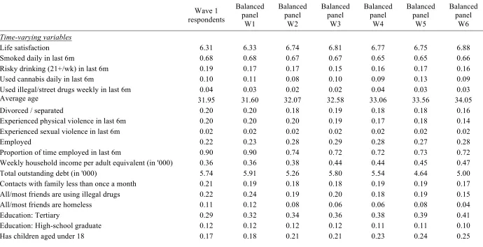
Of those 1,174 individuals in the balanced sample, 58% are men and 20% are from indigenous backgrounds. Around 25% of our sample spent some time in State care; 48% did not live with their parents when they were 14 years old because of parents’ divorce/separation, death or conflict with them; and 75% reported to have experienced emotional, physical or sexual abuse as a child; see Table A1 in the Appendix. Comparing to the average Australian population, the JH sample tends to consume significantly more addictive substances (Table 1). For example, in any particular wave, more than 65% of the JH sample smokes daily compared to 15.1% in the Australian population; and more than 30% uses cannabis and more than 10% uses illegal/street drugs compared to 14.7% in the Australian population (on average over all illegal drugs). Note that the JH sample does not consume alcohol at risky levels more often than the general population: approximately 15% for the JH sample compared to 20.1% in the Australian population.
3.2. Empirical Strategy
Our objective is to measure movements in individuals’ life satisfaction in periods before, during, and after the use of addictive substances. We have three main research questions:
(i) Is life satisfaction, as a measure of experienced utility, lower in periods preceding an individual’s consumption of addictive substances?
(ii) Is life satisfaction lower in periods in which respondents consume addictive substances?
(iii) Is past consumption of addictive substances correlated with lower life satisfaction in subsequent periods?
To implement our tests, we follow the method outlined in Frijters et al. (2011) and explore the leads and lags on substance use variables in life satisfaction equations. Assume that life satisfaction, LS, is a function of past, present, and future use of addictive substances, U, as follows:
LSit = β1Uit+1 + β2Uit + β3Uit-1 + γ’Xit + εit (1)
where i = 1,…, N; t = 1,…, T. The dependent variable, LSit, is standardised life satisfaction with a mean of zero and a standard deviation of 1. We define the lead “substance use” dummy, Uit+1 to take a value of 1 if the respondent uses a particular substance in period t+1 (i.e. in the 6 months following the interview in t), and a value of 0 if the respondent does not use in period t+1. Similarly, we define Uit to take a value of 1 if the respondent uses a particular substance in period t (i.e. in the 6 months preceding the interview in t), and a value of 0 if the respondent does not use that substance in t. Finally, we define Ut-1, to take a value of 1 if the respondent uses a particular substance in period t-1 (i.e., between one year and 6 months before the interview in t), and a value of 0 if the respondent does not use that substance in t-1. 8
her parents at age 14 because her parents were divorced/separated, was not living with her parents at age 14 because her parents were dead, was not living with her parents at age 14 because of conflicts, ever experienced emotional/physical/sexual abuse as a child, male caregiver (respectively female caregiver) had an alcohol or drug problem, male caregiver (respectively female caregiver) spent time in jail, male caregiver (respectively female caregiver) spent time in hospital because of mental health problems, male caregiver (respectively female caregiver) was unemployed for more than 6 months, male caregiver (respectively female caregiver) had a gambling problem. Note that these variables are excluded when we estimate individual fixed effects regressions.
We also include the following time-varying controls: wave fixed effects, age, age squared9, the proportion of time the respondent was employed in the last 6 months, weekly household income per adult equivalent (in thousands)10, total outstanding debt (in thousands), and indicator variables for whether the respondent: is divorced/separated, experienced physical violence in the last 6 months, experienced sexual violence in the last 6 months, was in employment in the last 6 months, has contact with her family less than once a month, all/most her friends are homeless, all/most her friends are using illegal drugs, graduated from high-school (Year 12 in Australia), has some tertiary education, and lives with children under 18. We also include dummy variables for missing control variables to avoid dropping observations that have missing information on some variables.
In order to account for individual unobserved heterogeneity, we also introduce individual fixed effects into the equation. Hence, the error term can be decomposed into the individual fixed effect component, φi, and the time-varying component, υit, as follows:
εit = φi + υit
us to control for path dependence in substance use (i.e., when respondents who use in one period are more likely to use in another period).
If individuals were significantly less satisfied with life prior to using drugs, then the coefficient on Uit+1 should be negative and statistically significant. The lead coefficient should, however, be statistically insignificantly different from zero if future usage is independent of how the individual is feeling about her life today. Both the RA model and the UM model predict that the marginal utility from future use should be negative or null.
The key distinction between the RA and the UM models is the prediction on the effect of current substance use on life satisfaction. If current use is associated with lower life satisfaction, then the coefficient on Uit should be negative – and even more negative than the coefficient on Uit+1. This would be consistent with the psychology model of UM, which predicts that consuming addictive substances that have harmful properties should lead to a significant deterioration of life satisfaction. However, if the coefficient on Uit is positive – or significantly less negative than the coefficient Uit+1 – then we have evidence that current consumption may have improved users’ life satisfaction compared to the previous period, which would be consistent with the prediction made by the RA model. Finally, both the RA and UM model predict that past substance use is associated with lower current life satisfaction. If this is the case and that this negative effect lasts at least 6 months, then the lag coefficient, captured by Ut-1, should be negative and statistically significant.
characteristics (Xit) as well as for individual fixed effects (i.e. all time-invariant characteristics). Although our controls are extensive, unobserved (time-varying) events in the respondents’ life may still bias our estimates.
Given that we have six waves of panel data, it is possible to follow individuals up to five survey waves before and after the use of drugs. To preserve a reasonable number of T in our fixed effects specification with both lead and lag coefficients estimated in the same regression equation (e.g., Frijters et al., 2011; Powdthavee, 2009b), we focus on life satisfaction: (i) just one period preceding substance use to identify the lead effect; and (ii) just one period following substance use to identify the lag effect.
All our estimations are done using either OLS or fixed effects linear models with cluster robust standard errors (clustered at the individual level) (Cameron & Miller, 2015).
4. Results
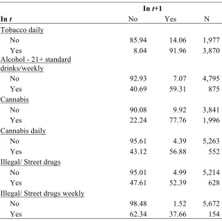
We begin our analysis by investigating the persistence in the consumption of our selected addictive substances. We present transitional matrices for each substance between periods t and t+1 in Table 2. The raw data suggests that smoking tobacco daily is the most persistent behaviour under study: 92% of individuals who reported to smoke daily in period t continued to smoke daily in period t+1. Smoking daily is also the addictive behaviour most frequently picked up whether again or for the first time: 14% of individuals who reported no daily use of tobacco in period t reported to smoke daily in period t+1. This is notably higher than for heavy drinking (21+ standard drinks per week) (7%); cannabis daily (4%); and illegal/street drugs weekly (2%). The second most persistent behaviour in our sample is consuming cannabis; 78% of respondents who reported to use cannabis in period t continued to use it in period t+1. Finally, only 38% of respondents who reported to use illegal/street drugs weekly in period t continued to use it weekly in period t+1. However, this could be due to other confounding factors, e.g., the environment and peers’ influences, rather than individual’s own preference to keep on using substances.
the regression, but in Column 4 all substances are entered together in the same regression.
Starting with the most parsimonious specification (i.e., controlling for only wave fixed effects) in Column 1 of Table 3 and focusing first on the lead effect, our estimates suggest that individuals report significantly lower life satisfaction in the periods that precede the daily consumption of tobacco (compared to periods that precede no/less than daily use), the daily consumption of cannabis (compared to periods that precede no/less than daily use), and the weekly consumption of illegal/street drugs (compared to periods that precede no/less than weekly use). The largest effect is observed for illegal/street drugs: individuals who consume illegal/street drugs weekly in period t+1 reported, on average, a 0.33 standard deviation lower life satisfaction.
As we include observable control variables in Column 2 of Table 3, two of the statistically significant lead coefficients – namely, tobacco and cannabis– become statistically insignificant. Introducing individual fixed effects in Column 3 increases rather than reduces the size of the estimated lead coefficient of illegal/street drugs. Finally, it makes virtually no difference to the estimated lead coefficient of illegal/street drugs whether or not all other substances were included together in the same regression.
The estimated lead coefficients imply that individuals experience a significant drop in life satisfaction up to 6 months before they start consuming illegal/street drugs on a weekly basis. On the contrary, there is little empirical evidence suggesting a drop in life satisfaction in the 6-months period preceding the consumption of tobacco daily, alcohol at risky levels, and cannabis daily once observed characteristics and individual fixed effects are accounted for in the regression.
2). However, by allowing for individual fixed effects in Column 3, the coefficient of smoking daily becomes statistically insignificant, whereas other coefficients on contemporaneous consumption continue to remain negative and statistically robust at least at the 5% level. Qualitatively similar results are also obtained in Column 4.
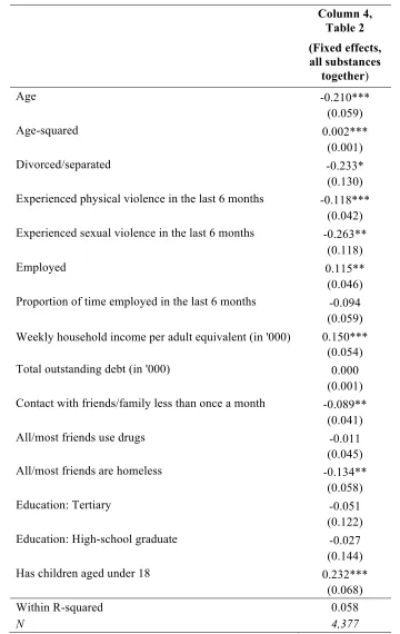
The estimated relationship between current substance use and life satisfaction is quantitatively important, especially for illegal/street drugs. Comparing it with other effect sizes obtained from the same specification (see Table A2 in the Appendix), we find that using illegal/street drugs weekly is equivalent to getting divorced or separating from one’s spouse. It is also equivalent to having experienced sexual violence in the last 6 months, and twice as negative as having experienced physical violence in the last 6 months.
It is worth noting that while we would like to interpret our estimated coefficients in t as causal, other interpretations are also possible. Individual fixed effects control for differences in characteristics that are either observed, or unobserved and invariant, but not for those that are unobserved and time-varying. Therefore, if some time-varying characteristics correlated both with life satisfaction and substance use are omitted from our specification (e.g., death of loved ones), our estimated coefficients may be biased upwards.
Turning to the lag coefficients of substance use in Table 3, only the lags of smoking daily and using illegal/street drugs weekly are (significantly) negatively correlated with current life satisfaction. This implies that, holding current consumption constant, daily smoking and using illegal/street drugs weekly in the previous period predict lower life satisfaction today.
While both lag coefficients continue to be negative and statistically significant with the inclusion of control variables (Column 2), the lag coefficient of daily tobacco use becomes statistically insignificant with the inclusion of individual fixed effects (Column 3). On the contrary, the lag coefficient of illegal/street drugs continues to be large, negative, and statistically well-determined, in a specification that conditions for both individual fixed effects and other types of addictive substances (Column 4).
In short, Table 3’s main results can be summarized as follows.
less satisfied individuals are more likely to consume addictive substances because of the expectation that by doing so, their experienced utility could improve.
• An excessive consumption of alcohol, the use of cannabis daily and illegal/street drugs weekly is observed together with a significant drop in life satisfaction. This finding is more consistent with the UM framework in which experienced utility is predicted to decrease in periods following individuals’ consumption of addictive substances.
• We find evidence that the consumption of illegal/street drugs 6 months to a year prior to the interview is associated with lower current life satisfaction, independently of current consumption. This suggests that of the substances studied, only illegal/street drugs may have an effect on life satisfaction for more than 6 months.
• Our results thus suggest a vicious circle of illegal/street drug use by which lower life satisfaction increases the propensity to consume illegal/street drugs that in turn further lowers life satisfaction in the future.
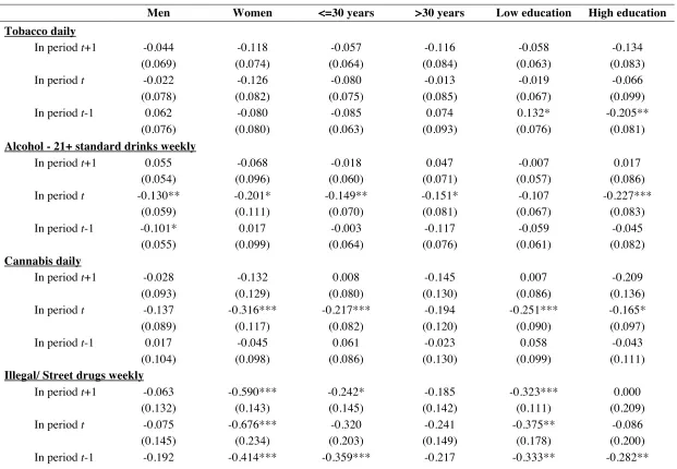
In Table 4 we test whether the results are qualitatively and quantitatively similar across gender, age groups, and education levels. We find some heterogeneity in the way individuals respond to substance use. Most notably, we find the estimated effects of past, present, and future consumption of illegal/street drugs on current life satisfaction to be noticeably more negative and statistically more pronounced for women and those from a lower educational background. Moreover, individuals from a high educational background tend to report significantly lower life satisfaction in periods following daily smoking, possibly related to the social stigma associated with smoking in highly educated circles.
adopted by Powdthavee (2009a, 2012) in the study of how disability and job loss indirectly shapes one’s life satisfaction through their effects on domain satisfactions.
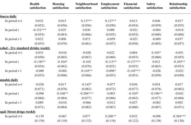
The most notable results are as follows. We find a significant drop in relationship satisfaction in periods preceding the use of illegal/street drugs, on average. Given that only women experience a drop in overall satisfaction before increasing their consumption of illegal/street drugs (Table 4), this result suggests that women’s intake of illegal/street drugs may be driven by dissatisfaction in their relationship. This is the largest lead effect out of all the drugs and domains, and is consistent with prior evidence that loneliness and social disconnectedness may contribute to substance use. On the contrary, individuals who become significantly more satisfied with their employment have a higher propensity for illegal/street drug use in the next period.
We find a significant drop in average health, safety and relationship satisfactions in periods in which respondents use illegal/street drugs, thus suggesting that the harmful effects of these drugs are fairly immediate and extend beyond the health domain. The estimated lag effects suggest that the previous consumption of illegal/street drugs is negatively associated with current life satisfaction possibly because it deteriorates neighbourhood and financial satisfaction.
With respect to other substances, the negative association between the use of cannabis daily in t and current life satisfaction (Table 3) is consistent with a contemporaneous decrease in neighbourhood, safety, housing and financial satisfaction. As for excessive alcohol use, the decrease in current life satisfaction is related to a decline in financial, health, employment, relationship and housing satisfaction.
5. Discussion
In the results discussed so far, we made a number of choices regarding the outcome variable, the substance use variables, the specification, the other control variables and the sample. These choices are extensively tested below and the results of these robustness checks demonstrate the robustness of our results.
One potential concern is that the use of an evaluative measure of wellbeing such as life satisfaction may not be the best representation of individuals’ experienced utility, especially compared to a measure of affective wellbeing, e.g., happiness, pain, boredom, etc. (Kahneman and Krueger, 2006). It is possible that individuals consume illegal/street drugs not to maximise their satisfaction with life as a whole, but rather to maximise their daily positive emotional experiences.12 However, this is not necessarily a strong objection. Indeed, if life satisfaction responses are correlated with what people think they should feel (or want) as well as how they currently feel (e.g., Schkade and Kahneman, 1998; Kahneman, 2011), life satisfaction still matters – and in many cases, matters more than affective wellbeing – as a predictor of future behaviours and outcomes (e.g., Benjamin et al., 2012; Clark, 2015). Life satisfaction therefore constitutes a valid policy outcome (Dolan et al., 2011) independent of affective wellbeing.
In response, we re-estimate our full specification using an alternative outcome, namely, the Kessler-6, which is a measure of psychological distress (standardised to a mean of 0 and a standard deviation of 1). Like other measures of mental wellbeing (e.g., the General Health Questionnaire (GHQ-12) and SF-36 mental health score), the Kessler-6 can be considered as a proxy measure of affective wellbeing, which is more related to an individual’s immediate conditions and experiences whereas life satisfaction is more related to one’s life goals (Kahneman & Krueger, 2006)13. It is
However, we find no association between the past and future use of illegal/street drugs and psychological distress. This is consistent with the use of illegal/street drugs being associated with intense dissatisfaction (as measured by psychological distress) in the short-run only but with more moderate forms of dissatisfaction (as measured by life satisfaction) for longer periods.
We also re-estimate our main specification (Column 4, Table 3) with alternative measures of addictive substances on the right-hand side. For example, we test whether our results are robust when we replace the alcohol variable with the following alternatives: 15 or more standard drinks weekly; binge drinking (number of bouts in month preceding interview); and quantity of drinking (average number of drinks per week). We find qualitatively similar results using those different definitions for alcohol use.14 Similarly, estimating the effects of the number of cigarettes smoked monthly, the number of days weekly in which cannabis is consumed (respectively illegal/street drugs), or a dummy for consuming cannabis (respectively illegal/street drugs) makes little difference to our results.
In addition, in a new specification, we consider four categories of users for each substance: abstainers (reference category), low users, medium users and high users (defined in tertiles of the distribution of use for each substance)15. While empirically demanding, this analysis allows us to identify more precisely the levels of use which constitute a tipping point in terms of life satisfaction, separately for each substance. The negative coefficient for alcohol abuse in t reported in Table 3 is mainly driven by the “high users”, i.e. respondents who report drinking 15 standard drinks or more weekly. The negative effect of cannabis in t comes from “medium users” and “high users”, i.e. respondents who use at least one day a week on average. The negative effect of illegal/street drugs in t is driven by all levels of use. In contrast, the effects of use in (t-1) and (t+1) come from high users only, i.e. respondents who use at least one day a week on average.
Arellano and Bover (1995), Blundell and Bond (1998), and more recently in an applied study of spouses’ SWB by Powdthavee (2009a), to arrive at an estimate which should be closer to the causal estimate of substance use. This process allows us to reduce the potential problem of reverse causality by which life satisfaction may modify respondents’ consumption of addictive substances and therefore bias our estimates upwards. The estimates obtained from the system GMM model are qualitatively very similar to those obtained using the fixed effects model, which implies that our original findings are robust to controlling for the lag dependent variable16.
Other potential concerns are the robustness of our results to alternative control variables, samples or specifications17. First, JH respondents exhibit more mental health issues than the general population (Scutella et al. 2012) and these could be related to both substance use and life satisfaction. Our estimates could therefore suggest that respondents’ substance use patterns don’t follow a pattern consistent with the RA model although in reality they do if mental health issues explain non-rational patterns of substance use. To test the implications of controlling for mental health issues, we add 5 dummy variables to capture whether the respondent was diagnosed with any of the following mental health conditions between interviews: bipolar affective disorder, schizophrenia, depression, post-traumatic stress disorder and anxiety disorder. Our results are largely unchanged. Note that more permanent mental health issues are controlled for by the individual fixed effects and should not bias our estimates. Our results also hold when adding dummies for the geographical location to control for local specificities. They are also similar when controlling for all variables in t-1 instead of t to minimise the possibility that we are over-controlling the channels by which substance use and life satisfaction are related.
Second, it might be argued that our findings, which are based on a balanced
Finally, our study also enables us to estimate the associated compensation variations (CVs) for the drops in average life satisfaction prior to and during the consumption of addictive substances. These CVs provide useful information about how much money it would take to restore the average wellbeing of the target population. Policy makers can then gauge an understanding of the level of damage addictive substances are causing individuals and design support programs appropriately.
Using the full specification (Column 4, Table 3), the estimated coefficient on weekly household income per adult equivalent (in $1,000) is 0.150 (S.E. = 0.054). This implies that an additional weekly income of AUD$1,500 is required to offset the drop in average life satisfaction that precedes the consumption of illegal/street drugs (i.e., (-0.225/0.150)*1000). To compensate the drop in average life satisfaction in the wave of reporting using illegal/street drugs requires AUD$1,853 per week (i.e., (-0.278/0.150)*1000). These large sums are indicative of the damage substance use causes in individuals’ lives and how expensive addictions may be for society, suggesting that prevention and rehabilitation programs may be cost-effective for society.
6. Conclusions
Economists have, over the years, built up a huge arsenal of empirical support for the notion that individuals have stable preferences and make utility-maximizing decisions about whether or not to consume addictive substances. Perhaps surprisingly, and likely due to economists’ mistrust of what people say, as opposed to what people do, relatively little research has been done to test whether or not measures of individuals’ experienced utility improve, as would be predicted by the rational addiction model, as a result of individuals making these rational decisions.
individuals tend to become even less satisfied with life – rather than more satisfied with life compared to the previous period – in the period of using illegal/street drugs. We find similar results for alcohol abuse and the daily consumption of cannabis. These results are consistent with the psychologists’ beliefs that the experienced utility resulting from a consumption decision may not match that of the decision utility. Indeed, this drop in average life satisfaction of substance users over the six months following the use of substances is less consistent with the RA model, but does not rule it out completely, provided that the use of substances increases individual’s life satisfaction in the very short term and that individuals have an extremely high discount rate. However, if individuals tend to overestimate the future beneficial effects of substance use on life satisfaction, then their behaviour is more in line with the UM model. Overall, our evidence suggests that the use of potentially harmful substances is likely to have a net negative wellbeing effect even in a very short term.
A feature of our analysis is to use reports on domain satisfactions to understand the potential underlying relationships between consumption of addictive substances and life satisfaction. For example, the current consumption of illegal/street drugs has the highest negative correlation with changes in relationship satisfaction, which also happens to be one of the larger predictors of life satisfaction. By contrast, the current excessive consumption of alcohol is estimated to have the highest negative correlation with changes in financial satisfaction, which ranks third in the order of determinants of life satisfaction. Knowing how different types of consumption are indirectly related to the overall life satisfaction is important. Indeed, it allows policy makers to make a more informed decision about which public policy – e.g., a policy on healthcare or a policy that improves social and financial supports for people addicted to drugs – they should be focusing their resources on to help substance users quit and improve the quality of life.
done on one of the most vulnerable groups of individuals in our society and may therefore not be representative of how individuals in a country might react to the consumption of hard drugs. Future research may have to return with a larger population sample to address this issue of representativeness.
References
Arellano, M. and Bover, O., 1995. Another look at the instrumental variable estimation of error-components models. Journal of Econometrics, 68(1), pp. 29-51.
Baltagi, B. H. and Griffin, J. M., 2002. Rational addiction to alcohol: panel data analysis of liquor consumption. Health Economics, 11(6), pp.485-491.
Becker, G. S., Grossman, M. and Murphy, K. M., 1991. Rational addiction and the effect of price on consumption. American Economic Review, 81(2), pp.237-241. Becker, G. S. and Murphy, K. M., 1988. A theory of rational addiction. Journal of
Political Economy, 96(4), pp.675-700.
Benjamin, D.J., Heffetz, O., Kimball, M.S. and Rees-Jones, A., 2012. What do you think would make you happier? What do you think you would choose? American Economic Review, 102(5), pp.2083-2110.
Blundell, R. and Bond, S., 1988. Initial conditions and moment restrictions in dynamic panel data models. Journal of Econometrics, 87(1), pp.115-143.
Brodeur, A., 2012. Smoking, Income and Subjective Wellbeing: Evidence from Smoking Bans. PSE Working Papers No. 2012-03, Paris: Paris School of Economics.
Cameron, A.C. and Miller, D.L., 2015. A practitioner’s guide to cluster-robust inference. Journal of Human Resource, 50(2), pp.317-372.
Cheng, T.C., Powdthavee, N. and Oswald, A.J., 2017. Longitudinal Evidence for a Midlife Nadir in Human Well-being: Results from Four Data Sets. Economic
Journal, 127(599), pp.126-142.
Chaloupka, F., 1991. Rational addictive behaviour and cigarette smoking. Journal of
Political Economy, 99(4), pp.722-742.
Clark, A.E., 2015. Is happiness the best measure of wellbeing? in M. Fleurbaey, M. Adler (eds.), Handbook of Wellbeing and Public Policy: Oxford University Press.
Clark, A.E., Diener, E., Georgellis, Y. and Lucas, R.E., 2008. Lags and leads in life satisfaction: a test of the baseline hypothesis. Economic Journal, 118(529), F222-F243.
Dolan, P., Layard, R. and Metcalfe, R., 2011. Measuring subjective wellbeing for public policy, The office for National Statistics, February.
Frijters, P., Johnston, D.W. and Shields, M.A., 2011. Life satisfaction dynamics with quarterly life event data. Scandinavian Journal of Economics, 113(1), pp. 190-211.
Gardner, J. and Oswald, A.J., 2006. Do divorcing couples become happier by breaking up?. Journal of the Royal Statistical Society: Series A (Statistics in Society), 169(2), pp.319-336.
Gilbert, D.T. and Wilson, T. D., 2000. Miswanting: Problems in affective forecasting. In J. Forgas (Ed.), Thinking and feeling: The role of affect in social cognition (pp. 178–197). New York: Cambridge University Press.
Grossman, M., 1993. The economic analysis of addictive behaviour. In: Bloss, G., Hilton, M. (Eds.), Economic and Socioeconomic Issues in the Prevention of Alcohol-related Problems. US Government Printing Office, Washington, DC, pp.91–124.
Grossman, M. and Chaloupka, F.J., 1998. The demand for cocaine by young adults: a rational addiction approach. Journal of Health Economics, 17(4), pp.427-474. Gruber, J. and Köszegi, B., 2001. Is Addiction “Rational”? Theory and Evidence.
Quarterly Journal of Economics, 116(4), pp.1261-1303.
Gruber, J. and Mullainathan, S., 2006. Do cigarette taxes make smokers happier? In Happiness and Public Policy, pp.109-146. Palgrave Macmillan UK.
Kahneman, D., Wakker, P.P. and Sarin, R., 1997. Back to Bentham? Explorations of
experienced utility. The Quarterly Journal of Economics, 112(2), pp.375-406.
Kahneman, D., 2011. Thinking, fast and slow. Macmillan.
Kahneman, D. and Deaton, A., 2010. High income improves evaluation of life but not emotional wellbeing. Proceedings of the National Academy of Sciences, 107(38), pp.16489-16493.
Kahneman, D. and Krueger, A.B., 2006. Developments in the measurement of subjective wellbeing. Journal of Economic Perspectives, 20(1), pp.3-24.
Kahneman, D. and Thaler, R.H., 2006. Anomalies: Utility maximization and
experienced utility. The Journal of Economic Perspectives, 20(1), pp.221-234.
Knabe, A., Rätzel, S., Schöb, R. and Weimann, J., 2010. Dissatisfied with Life but Having a Good Day: Time-use and Wellbeing of the Unemployed. Economic Journal, 120(547), pp.867-889.
Labeaga, J.M., 1999. A double-hurdle rational addiction model with heterogeneity: estimating the demand for tobacco. Journal of Econometrics, 93(1), pp.49-72. Laibson, D., 1997. Golden eggs and hyperbolic discounting. Quarterly Journal of
Economics, 112(2), pp.443-477.
Leicester, A. and Levell, P., 2016. Anti-smoking policies and smoker wellbeing: Evidence from Britain. Fiscal Studies, 37(2), pp.224-257.
Loewenstein, G., O'Donoghue, T. and Rabin, M., 2003. Projection bias in predicting future utility. Quarterly Journal of Economics, 118(4), pp.1209-1248.
Lucas, R.E., 2005. Time does not heal all wounds a longitudinal study of reaction and adaptation to divorce. Psychological science, 16(12), pp.945-950.
Lucas, R.E., Clark, A.E., Georgellis, Y. and Diener, E., 2004. Unemployment alters the set point for life satisfaction. Psychological science, 15(1), pp.8-13.
Odermatt, R. and Stutzer, A., 2015. Smoking bans, cigarette prices and life satisfaction. Journal of Health Economics, 44, pp.176-194.
O’Donoghue, T. and Rabin, M., 1999. Addiction and self control. Addiction: Entries and exits, pp.169-206.
Olekalns, N. and Bardsley, P., 1996. Rational addiction to caffeine: an analysis of coffee consumption. Journal of Political Economy, 104(5), pp.1100-1104. Oswald, A.J. and Powdthavee, N., 2008. Does happiness adapt? A longitudinal study
of disability with implications for economists and judges. Journal of public economics, 92(5), pp.1061-1077.
Powdthavee, N., 2009a. I can’t smile without you: Spousal correlation in life satisfaction. Journal of Economic Psychology, 30(4), pp.675-689.
Powdthavee, N., 2009b. What happens to people before and after disability? Focusing effects, lead effects, and adaptation in different areas of life. Social Science & Medicine, 69(12), pp.1834-1844.
Powdthavee, N., 2012. Jobless, friendless and broke: what happens to different areas of life before and after unemployment? Economica, 79(315), pp.557-575. Schkade, D.A. and Kahneman, D., 1998. Does living in California make people
Scutella, R., Johnson, G., Moschion, J., Tseng, Y. and Wooden M., 2012. Journeys Home. Research Report 1, Report prepared for the Australian Government Department of Families, Housing, Community Services and Indigenous Affairs. Shields, M.A., Price, S.W. and Wooden, M., 2009. Life satisfaction and the economic
and social characteristics of neighbourhoods. Journal of Population Economics, 22(2), pp.421-443.
Stutzer, A. and Frey, B.S., 2006. Does marriage make people happy, or do happy people get married? Journal of Socio-Economics, 35(2), pp.326-347.
Waters, T.M., and Sloan, F.A., 1995. Why do people drink? Tests of the rational addiction model. Applied Economics, 27(8), pp.727-736.
Wilson, T.D. and Gilbert, D.T., 2005. Affective forecasting knowing what to want. Current Directions in Psychological Science, 14(3), pp.131-134.
Wooden, M., Bevitt, A., Chigavazira, A., Greer, N., Johnson, G., Killackey, E., Moschion, J., Scutella, R., Tseng, Y-P. and Watson, N., 2012. Introducing “Journeys Home”. Australian Economic Review, 45(3), pp.368-378.
Yang, M. and Zucchelli, E., 2015. The impact of public smoking bans on wellbeing externalities: evidence from a natural experiment. Working Paper. Lancaster University, Department of Economics, Lancaster.
Table 1: Comparing the proportions of substance users between Journeys Home and the National Drug Strategy Household Survey
Tobacco - daily use
Alcohol - 21+ standard drinks/wk
Cannabis Illegal/ Street
drugs
Ever used over the survey period 77.3 34.7 55.6 29.2 Ever used on a regular basis over the survey
period - - 23.5 10.2
Always used over the survey period 48.4 3.1 14.9 1.9
Wave 1 - Spring 2011 68.1 17.0 38.6 12.9
Wave 2 - Autumn 2012 66.5 16.9 35.3 9.8
Wave 3 - Spring 2012 66.0 14.6 38.4 15.5
Wave 4 - Autumn 2013 65.4 16.1 34.0 10.6
Wave 5 - Spring 2013 64.4 16.5 34.6 12.0
Wave 6 - Autumn 2014 65.4 15.8 32.6 9.9
N 1,174 1,174 1,174 1,174
Australian population(2) 15.1 20.1 14.7
Table 2: Transitional matrix
In t+1
In t No Yes N
Tobacco daily
No 85.94 14.06 1,977
Yes 8.04 91.96 3,870
Alcohol - 21+ standard drinks/weekly
No 92.93 7.07 4,795
Yes 40.69 59.31 875
Cannabis
No 90.08 9.92 3,841
Yes 22.24 77.76 1,996
Cannabis daily
No 95.61 4.39 5,263
Yes 43.12 56.88 552
Illegal/ Street drugs
No 95.01 4.99 5,214
Yes 47.61 52.39 628
Illegal/ Street drugs weekly
No 98.48 1.52 5,672
Yes 62.34 37.66 154
Table 3: Standardised life satisfaction regressions with lead, current and lag consumption of addictive substances
Outcome: Standardised life satisfaction in t
(1) No controls (2) Observable controls (3) Individual fixed effects (4) Fixed effects, all substances together i) Tobacco daily
In period t+1 -0.098** -0.056 -0.066 -0.073 (0.045) (0.043) (0.047) (0.051) In period t -0.145*** -0.106*** -0.058 -0.052 (0.042) (0.041) (0.053) (0.056) In period t-1 -0.108** -0.088** -0.027 -0.008 (0.047) (0.044) (0.052) (0.056) N 4,661 4,661 4,661 4,377 ii) Alcohol - 21+ standard drinks weekly
In period t+1 -0.064 -0.001 0.021 0.016 (0.054) (0.049) (0.046) (0.048) In period t -0.215*** -0.137*** -0.157*** -0.150***
(0.050) (0.048) (0.054) (0.053) In period t-1 -0.069 -0.002 -0.074 -0.063 (0.051) (0.047) (0.049) (0.049) N 4,453 4,453 4,453 4,377 iii) Cannabis daily
In period t+1 -0.104* -0.028 -0.039 -0.063 (0.063) (0.060) (0.069) (0.074) In period t -0.268*** -0.135** -0.155** -0.193***
(0.058) (0.059) (0.068) (0.070) In period t-1 -0.071 0.014 0.027 0.019
(0.060) (0.061) (0.070) (0.076) N 4,621 4,621 4,621 4,377 iv) Illegal/ Street drugs weekly
In period t+1 -0.330*** -0.197* -0.235** -0.225** (0.109) (0.103) (0.092) (0.101) In period t -0.473*** -0.280*** -0.381*** -0.278**
(0.107) (0.100) (0.116) (0.130) In period t-1 -0.533*** -0.390*** -0.338*** -0.304***
(0.102) (0.098) (0.101) (0.111) N 4,631 4,631 4,631 4,377
Note: *<10%; **<5%; ***<1%. Robust standard errors – clustered at the individual level – are in parentheses.
“No control” specification includes only wave fixed effects.
[image:32.595.116.483.117.678.2]14, was not living with parents at age 14 because parents were dead at age 14, was not living with parents at age 14 because of conflicts, ever experienced emotional/physical/sexual abuse as a child, male caregiver (respectively female caregiver) had an alcohol or drug problem, male caregiver (respectively female caregiver) spent time in jail, male caregiver (respectively female caregiver) spent time in hospital because of mental health problems, male caregiver (respectively female caregiver) was unemployed for more than 6 months, male caregiver (respectively female caregiver) had gambling problem.
Table 4: Fixed effects standardised life satisfaction regressions by sub-sample
Men Women <=30 years >30 years Low education High education
Tobacco daily
In period t+1 -0.044 -0.118 -0.057 -0.116 -0.058 -0.134
(0.069) (0.074) (0.064) (0.084) (0.063) (0.083)
In period t -0.022 -0.126 -0.080 -0.013 -0.019 -0.066
(0.078) (0.082) (0.075) (0.085) (0.067) (0.099)
In period t-1 0.062 -0.080 -0.085 0.074 0.132* -0.205**
(0.076) (0.080) (0.063) (0.093) (0.076) (0.081)
Alcohol - 21+ standard drinks weekly
In period t+1 0.055 -0.068 -0.018 0.047 -0.007 0.017
(0.054) (0.096) (0.060) (0.071) (0.057) (0.086)
In period t -0.130** -0.201* -0.149** -0.151* -0.107 -0.227***
(0.059) (0.111) (0.070) (0.081) (0.067) (0.083)
In period t-1 -0.101* 0.017 -0.003 -0.117 -0.059 -0.045
(0.055) (0.099) (0.064) (0.076) (0.061) (0.082)
Cannabis daily
In period t+1 -0.028 -0.132 0.008 -0.145 0.007 -0.209
(0.093) (0.129) (0.080) (0.130) (0.086) (0.136)
In period t -0.137 -0.316*** -0.217*** -0.194 -0.251*** -0.165*
(0.089) (0.117) (0.082) (0.120) (0.090) (0.097)
In period t-1 0.017 -0.045 0.061 -0.023 0.058 -0.043
(0.104) (0.098) (0.086) (0.130) (0.099) (0.111)
Illegal/ Street drugs weekly
In period t+1 -0.063 -0.590*** -0.242* -0.185 -0.323*** 0.000
(0.132) (0.143) (0.145) (0.142) (0.111) (0.209)
In period t -0.075 -0.676*** -0.320 -0.241 -0.375** -0.086
(0.152) (0.135) (0.137) (0.176) (0.168) (0.116)
N 2,288 2,089 2,232 2,145 2,556 1,783
Note: *<10%; **<5%; ***<1%. Robust standard errors – clustered at the individual level – are in parentheses.
Table 5: Fixed effects domain satisfaction regressions with lead, current and lag consumption of addictive substances
Health satisfaction
Housing satisfaction
Neighbourhood satisfaction
Employment satisfaction
Financial satisfaction
Safety satisfaction
Relationship satisfaction
Tobacco daily
In period t+1 0.032 0.015 0.137** 0.127** 0.013 0.046 0.017
(0.052) (0.056) (0.056) (0.050) (0.054) (0.059) (0.055)
In period t -0.152*** 0.035 0.030 0.000 -0.021 -0.004 -0.018
(0.055) (0.063) (0.066) (0.055) (0.052) (0.060) (0.060)
In period t-1 0.022 0.008 0.073 -0.059 -0.021 -0.009 0.037
(0.053) (0.070) (0.061) (0.057) (0.056) (0.065) (0.057)
Alcohol - 21+ standard drinks weekly
In period t+1 0.033 -0.010 -0.020 0.022 0.004 0.105* -0.051
(0.050) (0.065) (0.067) (0.060) (0.053) (0.060) (0.055)
In period t -0.130** -0.104* -0.102 -0.115** -0.137*** 0.012 -0.105**
(0.054) (0.062) (0.070) (0.052) (0.053) (0.063) (0.053)
In period t-1 -0.080 -0.084 -0.145** -0.098* -0.145*** -0.026 -0.022
(0.053) (0.060) (0.066) (0.053) (0.051) (0.059) (0.049)
Cannabis daily
In period t+1 -0.028 0.017 -0.145* -0.077 0.036 0.024 0.017
(0.071) (0.078) (0.082) (0.072) (0.077) (0.078) (0.062)
In period t -0.098 -0.168** -0.206*** -0.003 -0.105* -0.196** -0.042
(0.066) (0.084) (0.077) (0.066) (0.062) (0.077) (0.068)
In period t-1 0.089 -0.018 -0.066 -0.012 0.027 -0.002 0.092
(0.071) (0.084) (0.082) (0.067) (0.066) (0.087) (0.071)
Illegal/ Street drugs weekly
In period t -0.235** -0.056 -0.075 -0.032 -0.130 -0.205* -0.256*
(0.115) (0.125) (0.103) (0.097) (0.108) (0.115) (0.133)
In period t-1 -0.150 -0.160 -0.418*** 0.042 -0.283*** -0.120 -0.114
(0.129) (0.116) (0.115) (0.102) (0.088) (0.127) (0.117)
N 4,379 4,377 4,354 4,152 4,372 4,354 4,353
Note: *<10%; **<5%; ***<1%. Robust standard errors – clustered at the individual level – are in parentheses.
Appendix
Table A1: Descriptive statistics
Wave 1
respondents
Balanced panel
W1
Balanced panel
W2
Balanced panel
W3
Balanced panel
W4
Balanced panel
W5
Balanced panel
W6
Time-varying variables
Life satisfaction 6.31 6.33 6.74 6.81 6.77 6.75 6.88
Smoked daily in last 6m 0.68 0.68 0.67 0.67 0.65 0.65 0.66
Risky drinking (21+/wk) in last 6m 0.19 0.17 0.17 0.15 0.16 0.17 0.16
Used cannabis daily in last 6m 0.10 0.11 0.08 0.10 0.09 0.13 0.09
Used illegal/street drugs weekly in last 6m 0.04 0.03 0.02 0.02 0.04 0.03 0.03
Average age 31.95 31.60 32.07 32.58 33.06 33.56 34.05
Divorced / separated 0.20 0.20 0.18 0.19 0.18 0.18 0.16
Experienced physical violence in last 6m 0.20 0.20 0.20 0.19 0.17 0.18 0.14
Experienced sexual violence in last 6m 0.02 0.02 0.02 0.02 0.02 0.02 0.02
Employed 0.22 0.23 0.28 0.29 0.28 0.27 0.28
Proportion of time employed in last 6m 0.90 0.90 0.74 0.72 0.72 0.73 0.72
Weekly household income per adult equivalent (in '000) 0.36 0.36 0.38 0.44 0.44 0.45 0.47
Total outstanding debt (in '000) 5.74 5.91 5.26 5.80 5.54 4.64 5.00
Contacts with family less than once a month 0.21 0.19 0.18 0.18 0.19 0.19 0.17
All/most friends are using illegal drugs 0.22 0.24 0.19 0.20 0.18 0.19 0.15
All/most friends are homeless 0.11 0.12 0.08 0.06 0.06 0.08 0.04
Education: Tertiary 0.29 0.32 0.34 0.36 0.38 0.39 0.41
Education: High-school graduate 0.12 0.12 0.12 0.12 0.11 0.11 0.10
Time-invariant variables
Male 0.59 0.58
Indigenous (including Torres Straight Islander) 0.22 0.20
Born in an English speaking country 0.92 0.92
Spent some time in State care 0.26 0.25
Did not live with parents at age 14 because
Parents were divorced/separated 0.33 0.34
Parents were dead 0.07 0.07
Of conflicts with parents 0.07 0.07
Experienced emotional abuse, physical or sexual violence
as a child 0.73 0.75
Male caregiver
Had an alcohol or drug problem 0.30 0.29
Spent time in jail 0.11 0.12
Spent time in hospital because mental health pbs 0.05 0.05
Was unemployed more than 6 m 0.18 0.16
Had a gambling problem 0.09 0.08
Female caregiver
Had an alcohol or drug problem 0.18 0.17
Spent time in jail 0.02 0.02
Spent time in hospital because mental health pbs 0.11 0.12
Was unemployed more than 6 m 0.42 0.43
Had a gambling problem 0.08 0.07
Table A2: Estimates of the control variables on standardised life satisfaction
[image:40.595.81.441.100.670.2]
Column 4, Table 2 (Fixed effects, all substances
together)
Age -0.210***
(0.059)
Age-squared 0.002***
(0.001)
Divorced/separated -0.233*
(0.130) Experienced physical violence in the last 6 months -0.118***
(0.042) Experienced sexual violence in the last 6 months -0.263**
(0.118)
Employed 0.115**
(0.046) Proportion of time employed in the last 6 months -0.094 (0.059) Weekly household income per adult equivalent (in '000) 0.150***
(0.054)
Total outstanding debt (in '000) 0.000
(0.001) Contact with friends/family less than once a month -0.089**
(0.041)
All/most friends use drugs -0.011
(0.045)
All/most friends are homeless -0.134**
(0.058)
Education: Tertiary -0.051
(0.122)
Education: High-school graduate -0.027
(0.144)
Has children aged under 18 0.232***
(0.068)
Within R-squared 0.058
N 4,377