Efficient indoor positioning with visual experiences via lifelong learning

warwick.ac.uk/lib-publications

Manuscript version: Author’s Accepted Manuscript

The version presented in WRAP is the author’s accepted manuscript and may differ from the

published version or Version of Record.

Persistent WRAP URL:

http://wrap.warwick.ac.uk/106567

How to cite:

Please refer to published version for the most recent bibliographic citation information.

If a published version is known of, the repository item page linked to above, will contain

details on accessing it.

Copyright and reuse:

The Warwick Research Archive Portal (WRAP) makes this work by researchers of the

University of Warwick available open access under the following conditions.

Copyright © and all moral rights to the version of the paper presented here belong to the

individual author(s) and/or other copyright owners. To the extent reasonable and

practicable the material made available in WRAP has been checked for eligibility before

being made available.

Copies of full items can be used for personal research or study, educational, or not-for-profit

purposes without prior permission or charge. Provided that the authors, title and full

bibliographic details are credited, a hyperlink and/or URL is given for the original metadata

page and the content is not changed in any way.

Publisher’s statement:

Please refer to the repository item page, publisher’s statement section, for further

information.

Efficient Indoor Positioning with Visual

Experiences via Lifelong Learning

Hongkai Wen

, Ronald Clark

, Sen Wang

, Xiaoxuan Lu

, Bowen Du

, Wen Hu

and Niki Trigoni

∗

_{Department of Computer Science, University of Warwick, UK}

_{Dyson Robotics Lab, Imperial College London, UK}

‡

_{Institute of Sensors, Signals and Systems, Heriot-Watt University, UK}

_{Department of Computer Science, University of Oxford, UK}

¶

_{School of Computer Science and Engineering, University of New South Wales, Australia}

Abstract—Positioning with visual sensors in indoor environments has many advantages: it doesn’t require infrastructure or accurate maps, and is more robust and accurate than other modalities such as WiFi. However, one of the biggest hurdles that prevents its practical application on mobile devices is the time-consuming visual processing pipeline. To overcome this problem, this paper proposes a novel lifelong learning approach to enable efficient and real-time visual positioning. We explore the fact that when following a previous visual experience for multiple times, one could gradually discover clues on how to traverse it with much less effort, e.g. which parts of the scene are more informative, and what kind of visual elements we should expect. Such second-order information is recorded as parameters, which provide key insights of the context and empower our system to dynamically optimise itself to stay localised with minimum cost. We implement the proposed approach on an array of mobile and wearable devices, and evaluate its performance in two indoor settings. Experimental results show our approach can reduce the visual processing time up to two orders of magnitude, while achieving sub-metre positioning accuracy.

Index Terms—Visual Positioning, Mobile and Wearable Devices, Lifelong Learning

F

1

I

The majority of indoor positioning systems to date represent a person’s location using precise coordinates in a 2D or 3D metric map, which has to be globally consistent. However, in many scenarios this could be an overkill: we don’t really need global maps to find a particular shop in the mall, as long as someone, e.g. the shop owners, could guide or “teach” us step by step. Therefore, we envision that in the future locations should be merelylabels, which are associated with objects, people, or other pieces of relevant information. In the same way as people exchanging mobile phone contacts, they can share locations, or to be more precise, the look and feel along the ways towards them, where others can ask their mobile phones or smart glasses to take them to “Jackie”, “Terminal 1” or “Mona Lisa”, by following navigation instructions extracted from previously constructed experiences.

Recently, this teach-repeat approach is gaining its popularity and has been implemented with various sensing modalities [1], [2], [3]. Comparing to the traditional solutions which seek to compute the global coordinates of the users [4], [5], [6], those teach-repeat systems require much less bootstrapping and training effort. For instance, the Escort system [1] navigates a user towards another by combining her previously recorded inertial trajectories with encounters from audio beacons. The FollowMe system [2] collects traces of magnetic field measurements as someone walks towards a destination, e.g. from the building entrance to a particular room. Later when another user tries to navigate to the same place, her position is estimated by comparing the live magnetic signal and step information with the stored traces. However in complex envi-ronments, the discriminative power of 1D sequence matching on magnetic field magnitude is limited. On the other hand, the

Travi-Corresponding author: Bowen Du, [email protected]

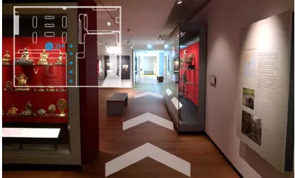
Fig. 1. The user interface of the proposed positioning system on smart glasses running in a museum environment.

Navi system [3] uses vision for teach-repeat navigation, which is promising since appearance is more informative than other modalities. In addition, with the emerging smart glass technology, vision-based solutions become more advantageous, since smart glasses are rigidly mounted on the head of the users, with cameras that are able to capture first-person point of view images (as shown in Fig.1). This is particularly useful in applications that require real-time and hands-free positioning, such as personal guidance for the visually impaired, remote assistance in industrial settings1_,

and augmented reality.

However in practice, achieving real-time visual positioning on mobile and wearable devices presents a number of challenges. Firstly, processing visual data can be prohibitively expensive for

Image Acquisition (~30ms)

Feature Detection (~6000ms)

Feature Quantisation (~8000ms)

BOW Comparison (~40ms)

[

]

...

[

]

[

]

[

]

[

]

0.02

0.89

0.01

Ref Imgs

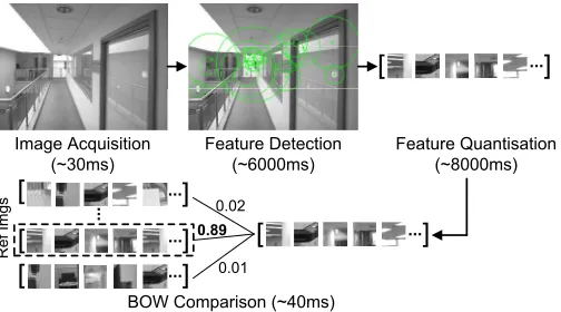
Fig. 2. Typical processing pipeline and running time (estimated on a Google Glass) of the Bag-of-Words image comparison approach [9].

resource constrained platforms. For instance, Fig. 2 shows a typical pipeline of the Bag-of-Words (BOW) image processing approach used by Travi-Navi. Given an image, the detected fea-tures are quantised into a vector of visual words (i.e. the scene elements) with respect to a pre-trained vocabulary. This BOW vector is then compared against a database of reference vectors, where the likelihood that two vectors represent the same scene is determined by certain distance metric. In our experiments we find that on the off-the-shelf smart glasses, just the feature detection and quantisation steps can take more than 10s to complete, which is impossible for real-time visual positioning. Some of the existing work [7] considers offloading the computation to the cloud, but it may not be cost-effective because: a) communication channels such as WiFi/4G are not always available or stable in some environments, e.g. construction sites; and b) the delay during localisation can be high due to different network conditions. The Travi-Navi system [3] bypasses this by only sampling images sparsely for pathway identification (not localisation), but this does not exploit the full power of visual positioning.

Our previous work [8] reduces the image processing time by pruning the visual vocabulary based on mutual information between words. However, such a global optimisation approach treats the entire environment equally, and doesn’t consider the ap-pearance variations across different locations. For instance Fig. 3 shows an example of images when following a previous visual experience in a museum. We see that place A is a large hall with many different visual elements, while the scene at place B contains much fewer, but more distinctive features. This means the optimal visual vocabulary for place B may not work at place A, since it may fail to include enough words to describe the complex scene there. On the other hand, when comparing images at place B, it is not necessary to consider the complete visual vocabulary as in A, but only a subset would be sufficient. Also comparing to A, most of the features in B are close to the camera, which can still be detected at lower resolutions. Thus at place B we can safely configure the camera to sample low resolution images to save processing time, but not vice versa. In addition, at place C most features are clustered on the left, and thus we can just process those parts instead of full images, which is not possible at A or B. In this paper, we aim to address the above challenges by moving away from the one-shotteach-repeatscheme, to a novel lifelong learningparadigm. The idea is that after following a visual experience across the space for several times, we can gradually learn visual processing parameters that are key to localisation success at different places, e.g. the minimum set of visual words,

C B

A

C B

A Previous

Experience

Current Experience

Fig. 3. Scene properties e.g. feature distribution and types of visual elements may vary significantly within a visual experience.

the lowest possible image scale, and the salient image regions. The learned knowledge is then annotated to the saved experiences as metadata, and is used to dynamically adjust the localisation algorithm when experiences are followed in the future. In this way, we can massively reduce computation on visual processing, where the positioning system only needs to process theminimum necessaryinformation to stay localised, and thus make real-time visual positioning possible. Concretely, the technical contributions of this paper are:

• We propose a novel lifelong learning paradigm, which infers key knowledge on how to follow previously collected visual experiences with minimum possible computation from sub-sequent repetitions. The learned parameters are annotated to the experiences, and are continuously improved over time. • We design a lightweight localisation algorithm, which

dy-namically adjusts its visual processing pipeline according to the annotated visual experiences. This allows us to build a positioning system that is infrastructure-free, requires little set-up effort, and runs in real-time on resource constrained mobile and wearable devices.

• We implement the proposed positioning system on various mobile phones and smart glasses, and evaluate it in two different indoor settings. Experiments show that comparing to the competing approaches, our system is able to reduce the running time up to two orders of magnitude, and achieve real-time positioning with sub-metre accuracy.

The rest of the paper is organised as follows. Sec. 2 provides an overview of the proposed approach. Sec. 3 explains how to learn optimal parameters for visual processing and annotate them to the experiences, while Sec. 4 presents the real-time localisation algorithm that takes the annotated experiences into account. Sec. 5 evaluates our system, and the related work is covered in Sec. 6. Sec. 7 concludes the paper and discusses possible future work.

2

O

Before presenting the proposed learning approach, in this section we first discuss our key assumptions on visual experiences and the problem of real-time localisation in Sec. 2.1, and then we describe the architecture of our positioning system in Sec. 2.2.

2.1 Model and Assumptions

Visual Experiences: A visual experienceE is a chain of nodes

(b) (a)

(ri , si , wi )

D

C B

A

ni

ei -1,i

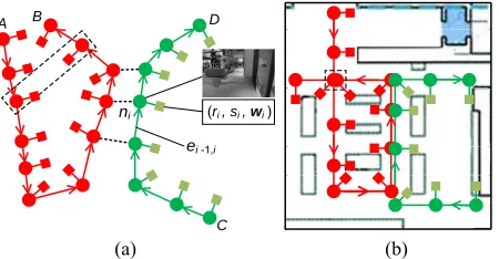
Fig. 4. (a) Two annotated experiences, where each node ni is as-sociated with visual processing parameters (ri, si,wi). The dashed lines are co-location links, through which the user can transit from one experience to another. (b) The global embedding of the annotated experience graph over the floorplan.

two nodes ni−1 and ni represents the metrical transformation between them, as shown in Fig. 4(a). In this work, ei−1,i is estimated using a pedestrian dead-reckoning (PDR) approach [11]. If multiple images are captured within one step, the edges be-tween them are computed by interpolation. Conceptually, a visual experienceE describes the appearance of the environment along the user trajectory towards a specific destination. Therefore when navigating to the same destination in the future, we can follow this experience E, by comparing the live images and motion measurements against those in E and work out where we are. It is also worth pointing out that an experience E doesn’t have to be globally consistent, e.g. it is well known that PDR suffers from long-term drift and the generated inertial trajectories may have accumulated errors (e.g. Fig. 4(a)). However as discussed later, our system only considersrelativelocalisation with respect to previous experiences, and thus as long as the user can follow those experiences locally, she can be successfully navigated to the desired destination step by step.

Visual Processing Pipeline: When following experiences, our system uses a Bag-of-Words (BOW) based [9] visual processing pipeline to process images. Without loss of generality, we use SURF [12] to extract image features, which are then quantised into vectors (i.e. bags) of visual words based on the pre-trained visual vocabulary. For instance, if the image contains a feature corresponding to a window, while thei-th word in the vocabulary represents a typical window (e.g. the average of different win-dows), then thei-th element of the generated BOW vector should be 1. Essentially the pipeline maps an image into a BOW vector, which describes the scene elements appear in that image, and the similarity between two images can be evaluated by the distance between their BOW vectors.

Visual Processing Parameters: At runtime, the cost of our visual processing pipeline is determined by two factors: the total volume of image pixels it has to process, and the amount of visual words to be compared with (see Fig. 2). Therefore, in this paper we consider the following parameters to configure the pipeline: a) the sampling image scale (i.e. resolution)rof the camera; b) the salient regionsof the captured image given the scaler; and c) the set of key visual wordswused by the pipeline to quantise image features. Intuitively,sandrtogether determine the cost of feature extraction step of the processing pipeline, while w governs the feature quantisation cost under the givensandr.

Annotated Visual Experience: In practice when following a pre-vious experience, it is not necessary to use the same configuration

for the visual processing pipeline throughout, since the appearance at different parts of the experience can vary significantly (as shown in Fig. 3). Therefore, we augment the visual experienceEto in-corporate the place dependent visual process parameters. For each nodeni ∈E, we attach the parameters (ri,si,wi), representing the optimal configuration of visual processing pipeline when the user is at the location ofni (as shown in Fig. 4(a)). In this way, the annotated experienceEdoesn’t only describe the appearance of a route across the workspace, but also specifies how we should follow it in different places. The ways of creating and updating the annotated experiences will be discussed in Sec.3 in more detail. Topometric Experience Graph: As the users continue to explore the indoor environment, our system uses atopometric experience graphto represent the saved experiences from different users, as shown in Fig. 4. In such a graph, each node has an Euclidean neighbourhood, but globally we assume no consistency. For exam-ple the two highlighted nodes in Fig. 4(a) are in fact at the same position (see Fig. 4(b)), but are represented differently due to the accumulated errors in inertial tracking. We also exploit the spatial overlapping between experiences by creating undirected links between nodes with similar visual appearance. Those co-location links increase the connectivity of the graph, from which one could transit between different experiences. For instance, in Fig. 4(a), to go from A to D, one could start with the experience on the left, then transit to the experience on the right via any co-location link, and follow it afterwards. Note that it is straightforward to use other sensing modalities, such as WiFi or Bluetooh beacons, to create co-location links [13], if a reliable similarity metric is provided. Localisation with Visual Experiences: We consider relative localisation, where at a given time, the location of the user is specified by a pair (ni, T). ni is the node in the experience graph that is the closest to the current user position, and T is the user’s relative displacement fromni. Intuitively, we match the observed sensor measurements with those in the experience graph to “pin down” the user, and then use the motion data to track her accurate position with respect to matched node. Therefore in our context, localisation is not performed in a globally consistent map, but only the topometric experience graph which can be viewed as a manifold [10]. This is particularly useful in navigation scenarios, where our system can just localise the users within the experience graph and navigate them to their destinations, without the expensive process of enforcing a global Euclidean map. On the other hand, if the graph can be embedded to a consistent frame of reference, e.g. by map matching [6], localisation against the graph is equivalent to positioning within the global map (see Fig. 4(b)).

The problem tackled by this work is how to make such localisationefficient, and run inreal-timeon resource constrained mobile and wearable devices. To address this, we propose a positioning system that continuously learns the optimal visual processing parameters (i.e.ri,siandwi) from localisation results, and annotates the learned parameters to the previous experiences. When being tasked later, our system actively tunes the visual processing pipeline according to such knowledge, to stay localised with minimum possible computation. Now we are in a position to explain the architecture of the proposed system.

2.2 System Architecture

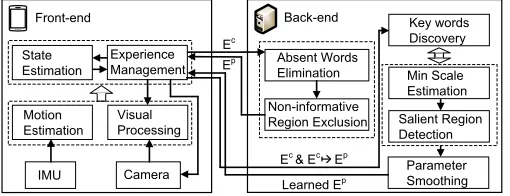
Fig. 5 shows the architecture of the proposed positioning system, which consists of a front-end that runs on the mobile devices, and a back-end which resides on the cloud.

Front-end Back-end

Motion Estimation

Visual Processing State

Estimation

Camera IMU

Experience Management

Key words Discovery

Salient Region Detection

Min Scale Estimation Absent Words

Elimination

Non-informative Region Exclusion Ec

Ep

Learned Ep Ec _{& E}c _Ep

Parameter Smoothing

Fig. 5. The architecture of the proposed system, where the front-end runs on the user carried devices, and the back-end resides on the cloud.

sensor observations. In practice, it is possible to localise with respect to more than one experiences, i.e. the sensor observations can be matched to co-located nodes from different experiences, but for simplicity here we only localise using the best matched experience in the graph. LetEp be the experience, andni ∈Ep be the node that the user is currently localised to. Then the live frame is passed through the visual processing pipeline, which is adjusted according to the parameters encoded inni. The matching results is then fused with measurements from IMUs, and the user position is determined by a state estimation algorithm. At the meantime, the front-end saves the current experienceEc by logging the live images and motion data, which will be used by the back-end later. We consider a motion-guided image sampling strategy as in [8], while the sampling rate depends on the accuracy requirement and energy budget set by the users (typically<1Hz). When localisation fails, i.e. the user can no longer be localised within the current experiences, the front-end pauses the state estimation process and only saves the observed sensor streams as a new experience En_{, until localisation can be reinstated.} In practice, such localisation failure would occur if the user starts to explore a new route that hasn’t been covered by exiting experiences, or when the appearance of a previously traversed route has changed dramatically, e.g. due to variations in lighting. Note that in our system, we tend to record denseEn_{by sampling} images at a much higher rate, to build an initial survey of the new environment/appearance. In typical indoor environments, this process won’t happen frequently, and the experience graph tends to converge as more experiences are accumulated.

Back-end: Once the user finishes following a previous experi-enceEp _{(assuming it has been annotated with visual processing} parameters), the current experienceEc_{and the localisation results,} i.e. the mapping between nodes inEc _andEp _{will be uploaded} to the back-end for learning when appropriate, e.g. the device is charged and/or connected to WiFi. If a new experienceEn _has been created, e.g. the user has just explored a new trajectory, the saved En _{will also be uploaded. In the former case, the} back-end iteratively computes the minimum key word set wi, the optimal image salient region si and scale ri, with which the correspondence betweenEc _andEp _{can still be maintained.} The learned parameters are used to update those inEp_{, and are} referred to by the front-end when the user is localised against

Ep _{in the future. On the other hand, given the new experience}

En_{, for each node n}

i ∈ En, the back-end computes the initial estimates of the visual processing parameters by pruning the redundant visual words and non-informative image regions (details will be discussed in Sec. 3.1). Then it assembles the annotated experience to the experience graph by exploiting co-location links (e.g. as in our previous work [13]), where the updated graph will

be downloaded and used by the front-end in next localisation. In practice, the above experience annotation process runs on the cloud infrastructure or local cloudlet [7], which typically have sufficient computational power to handle the overhead. In addition, our system doesn’t require real-time experience annotation or constant communication between the front-end and back-end. When the annotated experiences are ready and downloaded to the front-end, it can operate without the cloud. Therefore, in our system localisation performance won’t be affected by network latency, which is very desirable in practice.

In this way the proposed system forms a feedback loop, which doesn’t just learn about the indoor environment for once and then localise the users with this one-shot learned experiences, but also continuouslylearns fromthe subsequent traversals to improve itself and work smarter over time.

3

E

A

This section discusses the proposed approach of experience an-notation, which continuously learns how to configure the visual processing pipeline to achieve more efficient localisation in the future. As discussed in Sec. 2.1, the computational bottleneck of visual processing is the feature extraction and quantisation steps (see Fig. 2), whose cost is determined by: a) the total volume of pixels one has to process; and b) the amount of visual words to be compared against. For a given nodeniin an experience, the former is actually the size of the salient regionsi under the image scale

ri(denoted as|si|ri), while the latter is the cardinality|wi|of the key word set. Therefore our goal is to find the set of parameters

ri,siandwi, which yield the minimum possible|si|ri and|wi|. In Sec. 3.1, we first discuss how to compute the initial estimates of the parameters given a newly created experience. Then in Sec. 3.2 we show how the parameters can be continousely optimised by learning from subsequent repetition of the experiences.

3.1 Parameter Initialisation

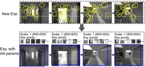
As discussed in Sec. 2.2, when the user explores a trajectory for the first time, or the appearance of a previously traversed route has changed significantly, the front-end creates a new visual experienceEn _{and upload it to the cloud when communication is} available. At this stage, our system tries to compute good initial estimates of the visual processing parameters by exploiting the scene properties at different parts ofEn_{(as shown in Fig. 6).}

3.1.1 Eliminate Absent Visual Words

New Exp.

Exp.with init params

Scale: 1 (800×600)

Key words: Scale: 1 (800×600) Scale: 1 (800×600) Scale: 1 (800×600) ... Key words: ... Key words: ... Key words: ...

Fig. 6. For a newly created experience, the proposed system estimates the initial parameters by pruning unnecessary information.

Based on this intuition, for each nodeniin the newly created visual experienceEn, we initialise the key word setwias follows. We consider a sliding window of 2k nodes [ni−k+1, ..., ni+k] centred atni. The images within the window are fed to the visual processing pipeline, where features are extracted and quantised into Bag-of-Words vectors with the original visual vocabulary. Assuming the vocabulary contains N visual wordsw1, ..., wN. Then the window of images can be represented as a 2k×N

matrixF. Each rowF(l,:)represents a particular image, and the

n-th elementF(l, n) is the frequency that wordwn appears in that image. Finally, whether the word wn should be included in the key word setwiis given by the indicator function:

1(wn) =



   

   

1,

i+k P

l=i−k+1

F(l, n)>0 0,

i+k P

l=i−k+1

F(l, n) = 0

(1)

This effectively rules out the visual words that never present within the neighbourhood of an experience nodeni, and selects a much smaller set of key words that have to be compared against, as shown in Fig. 8(a) and (b).

3.1.2 Prune Non-informative Image Regions

In addition to removing the unseen visual words, at this stage our system also tries to find a smaller salient region si for the image stored in nodeni. Note that here we keep the image scale

ri unchanged, because for now we are unable to determine the minimum possible ri for successful localisation with respect to the experienceEn _{(we will show how to learn the optimal scale}

riwith more experiences in the next section). Concretely, for each nodeniour system tries to locate the image patches containing no features (e.g. the slice of white wall in the first image of Fig. 6), or only the non-informative features (as discussed below), and eliminate those patches from the salient regionsi.

Letfkbe an extracted feature of the image in nodeni. During the image quantisation step, for each wordwn in the vocabulary, we compute the distance between featurefk and word wn. Then fk is quantised to the word with the smallest distance, indicating that fk belongs to the same type of visual element represented by that word. Letd(fk)be the smallest distance when quantising featurefk.d(fk)indicates how well the featurefkcan be described with the current vocabulary. In practice, larged(fk)means that the vocabulary doesn’t contain visual elements similar to the feature fk, i.e. we are not sure what fk represents. For instance, the highlighted feature in the third image of Fig. 6 is the reflection of a light on the window, which can’t be well represented by the current visual vocabulary. As a result, such a feature won’t contribute to

Scale: 1 (800×600)

Key words: Scale: 1 (800×600) Scale: 1 (800×600) Scale: 1 (800×600)

... Key words: ... Key words: ... Key words: ...

Current Exp.

Scale: 0.2 (160×120)

Key words: Scale: 0.4 (320×240) Scale: 0.4 (320×240) Scale: 0.2 (160×120)

... Key words: ... Key words: ... Key words: ... Exp.with

init params

Exp.with opt params

Fig. 7. Given the localisation results, our system updates the experience annotations by learning the optimal parameters for visual processing.

the BOW matching process but could introduce noises. Therefore, our system prunes those features and set the initial salient region

si according to the bounding box of the rest visual features (as shown in Fig. 6). In practice, we typically set the initialsi to be slightly larger than the bounding box, to account for potential view point changes when following the experienceEn_{. In addition, if} the computed bounding box is too small comparing to the image dimension (in our experiments we consider <50%), e.g. when images contain very few informative features due to blurriness, we set the initialsias the original image size for now and leave it to the later learning stage.

After the above initialisation process, the newly created expe-rienceEn _{has been annotated with the initial estimates of visual} processing parameters. As discussed in Sec. 2.2, this annotated experience will be assembled to the experience graph through co-location links, and downloaded to the user devices when it is needed for future localisation.

3.2 Lifelong Parameter Learning

With the initial estimates of the visual processing parameters, our system is able to exclude some unnecessary information during image processing, e.g. the redundant visual words or non-informative images regions. This can already reduce the runtime cost when following the experiences. However in many cases, we could further improve performance by learning from the subsequent repetitions of the previous experiences, just like what humans would do. For instance, when we first follow someone along a trajectory, we tend to stay alert throughout and watch out for as many visual clues possible. However after a few more traversals, we become more familiar with the route, and will discover place-dependent information that is vital for localisa-tion/navigation success, e.g. in some places we may only need to pay attention to a few landmarks to keep on the right track. Follow this intuition, our system employs alifelong learning paradigm, which keeps calibrating the optimal visual processing parameters through continued use.

All words

All nodes in exp.

w1 w2 ... wN

n1 n2

nM

...

ni

...

(a)

Nodes within 2k sliding window in exp.

w'1w'2 ... w'N'

ni-k+1

...

ni

...

(b)

Present Words

ni+k

Nodes within 2k sliding window in exp.

w'1w'2 ... w'N'

ni-k+1

...

ni

...

(c)

Present Words

ni+k

...

Discriminative words

Live image Live image Live image

Fig. 8. During localisation, a live image can be compared with (a) all nodes using the complete vosual vocabulary (stanrdard approach); (b) a sliding window of nodes using only the present words (after parameter initialisation); and (c) the most discriminative words (after parameter learning).

experiences Ec _{7→ E}p_{. Note that here the visual processing} parameters encoded in Ep _{can be either computed by the} ini-tialisation step as above, or from the previous learning iteration.

In our case, the goal of the learning process is to compute the optimal visual parameters(ri, si,wi)given the known correspon-dence between experiencesEc _7→Ep_{, which are the solution of} the following constrained optimisation problem:

minimize ri,si,wi

|si|r_i,|wi|

subject to p(hj 7→ni|Ep, ri, si,wi)≥,

hj ∈Ec, ni∈Ep

p(hj 7→ ni|Ep, ri, si,wi) is the likelihood that the image in node hj matches that of ni given the current parameters, and is evaluated with the FAB-MAP [14] approach. The constraint requires the matching likelihood of hj toni exceed a threshold

. In out implementation we typically require > 0.5, so that in the majority cases the nodehjshould be correctly matched to nodeni. Intuitively,|si|r_i and|wi|in the objective function are correlated. Images at lower scale or with smaller salient region (i.e. smaller|si|r_i ) tend to contain fewer visual features, and thus could require a sparser key word set to quantise. On the other hand, if just a few words are essential for correct matching, we can work at lower image scales, and/or only on image patches corresponding to those key words. Therefore, the proposed system optimises the two parts of the objective function iteratively. In each iteration, we first find the set of key visual words wi that are vital for successful matching (Sec. 3.2.1). Then given the computed wi, we estimate the salient regionsi together with the suitable scale

ri (Sec. 3.2.2). In the next iteration, the estimatedri andsi are used to evaluate a new key word setwiaccordingly. This process terminates when the parameters(ri, si,wi)converge, or a certain number of iterations has been reached. In practice, it is possible that before the learning process the matching likelihoodp(hj 7→

ni|Ep_{, r}

i, si,wi)is already below the threshold. In those cases, our system resets the parameters to their initial values and starts learning from there. Finally, the learned parameters are smoothed within a local neighbourhood to improve robustness and account for spatial correlations (Sec. 3.2.3). Now we are in a position to explain the optimisation steps in more detail.

3.2.1 Discover the Most Discriminative Visual Words

For each node ni in the previous experience Ep, the key word set wi has been initialised as the words that appear within its neighbourhood of 2k nodes, as discussed in Sec. 3.1.1 (see

Fig. 8(b)). Given the known mappinghj 7→ ni (from the local-isation results), our system further reduces wi, to only include the most discriminative words, with which the images in nodes

hj andni can be matched. For instance, in our experiments we found visual elements representing the carpet tiles are common in most of places, which contribute very limited discriminative power when matching images, and thus should be excluded from the key word set. Therefore, we wish to find a minimumsubset of the current key wordswiso that the mappinghj 7→ni holds. In this process, our system also considers a sliding window of 2k

nodes, and works as follows. Firstly, with the current parameters

(ri, si,wi), the images within the window are processed into Bag-of-Words (BOW) vectors. Assuming the current key word set contains N0 visual wordsw0₁, ..., w0_N0. Like in the previous

Sec. 3.1.1, here we also consider a 2k×N0matrixF0to represent the images in BOW format, whose elements are the frequency of words. For a given wordwn0, we define its discriminative power within the 2kwindow as:

H(w0n) =− i+k X

l=i−k+1

F0(l, n) lnF0(l, n) (2) In fact, if we normalise the n-th column F0(:, n) into a distri-bution, the above H(w_n0) is essentially itsinformation entropy. Intuitively, the wordw0_nthat only appears in a few images is more promising to distinguish them from the others. In this way, by ranking the entropyH(wn0)(i.e. discriminative power of words), we obtain a ranked word setw*i.

Finally, our system evaluates a new key word setw0_ibased on the computed *wi. Conceptually, this can be done by iteratively adding words tow0_i, until the node hj can be reliably matched to ni. To speed up this process, we initialise w0_i as the first half of ranked set w*i (those are more informative), while the rest is considered as a candidate set. Then in each iteration, we use the current w0_i to compare the image of hj against those within the sliding window, and evaluate the matching likelihood

p(hj 7→ni). Ifp(hj 7→ni)exceeds, we reducew0i by half in the next iteration; otherwise we move the first half of the words in the candidate set to w0_i. After at most log2|

*

(a) (b)

ni∈ Ep ni∈ Ep

hj0.25: p = 0.03

hj0.5: p = 0.51

hj1: p = 0.95

hj0.25: p = 0.53

hj0.5: p = 0.72

hj1: p = 0.99

hj∈ Ec hj∈ Ec

Fig. 9. Matching results of image pyramids for cases where dominating features are (a) far away from; and (b) close to the camera. Blue bounding boxes illustrate the estimated salient regions at different layers.

shown in Fig. 8(c)). In Sec. 5, we will show that comparing to the standard approach, using the minimum key words sets in localisation could reduce up to 80% of feature quantisation cost.

3.2.2 Detect Salient Regions at Multiple Scales

Now we show how to further minimise the total amount of pixels |si|r_i to be processed given the current key word setwi.|si|r_i is a function of the sampling image scale ri and the salient regionsi, and has direct impact on the cost of feature extraction and quantisation. Intuitively,ri indicates the level of detail one should consider, e.g. if most of the visual features are close to the camera (see Fig. 9(b)), it would be sufficient to sample images at lower scales to maintain the correct mapping. On the other hand, under a fixed scale ri, the dominating visual elements may be well clustered within certain salient region si, e.g. as shown in Fig. 9(b), most of the informative features are within the top left part of the image. Therefore, if we assume the device’s point of view remains relatively stable, when localising against previous experiences, it is sufficient to sample live images at the lowest possible scales and only process the smallest salient regions.

Our system considers a progressive approach to evaluate the optimalri andsi for eachni ∈ Ep. Lethj ∈ Ec be the node matched toni. We first create an image pyramid forhj by down-sampling at different scales. Fig. 9 shows an example of image pyramids with three layers, where the lowest layerh1

j contains the original image (scale 1), and top two layers contain images at scale 0.5 and 0.25 respectively (i.e. 1/4 and 1/16 in size of the original image). In practice, the scales of the pyramid are determined by the camera hardware (e.g. limited by the supported sampling resolutions), and the number of layers can be tuned for different environments. Then fromh1

j upwards, images at different scales are passed through the visual processing pipeline, and compared with images in the previous experienceEp_{. To capture the scene} variations in different parts of Ep_{, we also consider a sliding} window of 2knodes centred atni. In addition, our system only uses the learned key word setwi for image quantisation, where visual features do not appear inwiare pruned.

At the layer with scaler, if the likelihoodp(hr

j 7→ni)exceeds the threshold, we further try to estimate the salient image region. Concretely, our system initialises the candidate salient regionsin the same way as discussed in Sec. 3.1.2, and then reduces its size by removing features insiteratively. Letf1, ...,fK be the set of features left in the current iteration. For simplicity, we assume a featurefk can be represented as an image patch (e.g. the circles in Fig. 9), and the current salient regions is the bounding box containing all the K features. For each feature fk, we evaluate the gain and residual if it is removed from the current feature

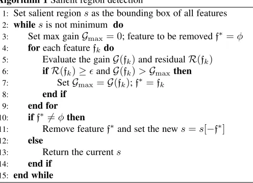
Algorithm 1Salient region detection

1: Set salient regionsas the bounding box of all features

2: whilesis not minimum do

3: Set max gainGmax= 0; feature to be removedf∗=φ

4: foreach featurefkdo

5: Evaluate the gainG(fk)and residualR(fk)

6: ifR(fk)≥andG(fk)>Gmaxthen

7: SetGmax=G(fk);f∗=fk

8: end if

9: end for

10: iff∗6=φthen

11: Remove featuref∗and set the news=s[−f∗] 12: else

13: Return the currents

14: end if

15: end while

set. Let s[−fk] be the hypothetical bounding box if feature fk is removed. We define the gain of removing fk as the reduced amount of pixels between the hypothetical and current bounding boxesG(fk) = |s| − |s[−fk]|(Line. 5 in Algo. 1). On the other hand, the residualR(fk)of excludingfkis defined as the mapping likelihood evaluated using features withoutfk. Then we loop over all features and try to remove the one with the highest possible gain, whose residual is still beyond the threshold. If such afk exists, the salient region is updated tos[−fk]and we proceed to the next iteration. Otherwise the currents is already minimum, and the algorithm terminates. The detailed algorithm of salient region detection is shown in Algo. 1.

In this way, our system processes each layer of the image pyramid and stops when it reaches the highest layer where the mapping likelihood exceeds . This means there is no scope to further reduce |si|r_i any more, and the learned si and ri are considered to be optimal. In practice, the estimated si and ri could vary across different parts of the experience. For instance, in Fig. 9(a) the estimated salient region is at scale 0.5, while that in Fig. 9(b) is at scale 0.25 (∼4 times smaller). This is because in the scene of Fig. 9(a), most of the features are quite far away from the camera, and would disappear when considering lower scales. On the other hand, in Fig. 9(b) most of the features are relatively close, and thus images at lower scales can still be reliably matched.

3.2.3 Smooth the Learned Parameters

xt-1 xt xt+1 u1:T

vt-1 vt

…

vt+1

fu(xt-1, xt, ut)

fv(xt, vt)

…

...

pn1

t+1

pnM

t+1

(d1, θ1)

(dt, _... θt)

...

fθ(xt, θt-ω,t )

Fig. 10. The CRF model used in the proposed system.

under optimal scaleri, and|I|is the original image size. Similarly, the complexity of feature quantisation can also be reduced at least by a factor of|wi|/ N, where|wi|is the number of words in the learned vocabulary, whileN is the size of the initial vocabulary.

However, as discussed in Sec. 2.2, when following a previous experienceEp, to reduce energy consumption the current experi-enceEc saved by the front-end typically contains sparser nodes than Ep. This means in one learning iteration we could only update the parameters in some of the nodes inEp. In addition, although those learned parameters are considered to be optimal for localisation, they reduce the information quite aggressively. In practice we want to increase the stability of our system, and avoid adjusting the visual processing pipeline too often. Therefore, our system also applies a smoothing process at the end of each learning iteration.

Let us consider the 2knodes centred atni in the experience

Ep_{. Suppose that through the learning process, we have updated} the parameters in a subset of nodesNnew

i within the 2kwindow, while the parameters associated with the rest of the nodes Nold

i remain unchanged. LetWnew

i be the union of the key words of the newly updated nodesNnew

i , whileWiold be the set of words that appear in the 2kwindow but not inWnew

i . We first let the key word setwiof the nodenito beWinew, and then add the topq% words inWold

i based on how frequent they appear. In this way, we guarantee that the key words discovered through the learning iteration is included, while also keep some common key words appeared in the neighbourhood. For the image scaleriand salient regionsi, we consider a weighted voting/average scheme within the 2k window. We typically assign more weight to the newly learned parameters, i.e. those associated with nodes inNnew

i , and then use a Gaussian kernel to take the spatial correlations into account. Therefore with the smoothed parameters, when localising the users with respect to the previous experiences, the proposed system is less prune to environmental dynamics e.g. view point changes caused by head movement, and can achieve better trade-off between computational efficiency and robustness.

4

L

A

E

4.1 Conditional Random Fields (CRFs)

In this section, we present the design and implementation of the proposed localisation algorithm, which is used by the front-end of our system to position the users with respect to the previously annotated experiences, as discussed in Sec. 2. Let us assume that a user is following an annotated experienceEp_{, which has been} downloaded to her mobile device already. To position the users in real-time on resource constrained mobile and wearable devices,

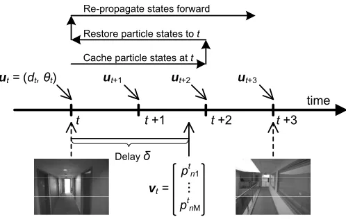
ut = (dt, θt)

t t +1 t +2 t +3

time

pt n1

...

pt nM

ut+1 ut+2 ut+3

Delay δ

Restore particle states to t

Re-propagate states forward

vt = Cache particle states at t

Fig. 11. The proposed system handles the delayed visual measure-ments by rolling back to particle states when the images were taken, and re-propagating the states with the user motion observed afterwards.

the localisation algorithm has to be extremely lightweight, and able to cope with the delay of visual processing (see Fig.11). To address this, our system models the position of user with respect to the previous experienceEp_{as the latent states, and considers} a delay-tolerant sequential state estimator to fuse the inertial and visual data. In particular, we consider the undirected Conditional Random Fields (CRFs), because they are more flexible in handling correlated measurements from heterogeneous sensing modalities.

Latent States: As discussed in Sec. 2.1, the position of the user

xtcan be represented as a pair(ni, T)whereni is the node in

Ep that is the closest, andT is the relative transformation from the position ofnitoxt. In practice,T can be estimated from the motion/odometry data, and thus localisation against the previous experience Ep can be cast into that of finding the matching nodes in Ep that can best explain the sensor measurements. Therefore, in this paper we define the state space as the set

visual measurements later on.

Visual Measurements: Unlike the existing systems such as Travi-Navi, our visual processing pipeline is configured dynam-ically according to the current state belief and experience annota-tions. Letxt=nibe the predicted state at timet. We retrieve the parameters(ri, si,wi)annotated to nodeni, and task the camera to take an image at scale ri. Then only features appear within the salient regionsi are extracted, and quantised into a Bag-of-Words vector according to the key word setwi. Finally, the BOW vector is compared with the images of the previous experienceEp_. Therefore, the visual measurement at timetallows us to derive a distributionvt= [ptn1, ..., p

t

nM](as shown in Fig. 10), wherep t nk is the likelihood that the captured image matchesnkinEp.

4.2 Feature Functions

In our model the conditional dependencies between states and observations can be factored as products of potentials:

p(x1:T|u1:T,v1:T) =c−1· T Y

t=2

Ψ(xt−1, xt,u1:T,v1:T) (3)

c is a normalising constant, which integrates over all state se-quences:c =R Q

Ψ(·)dx1:T. The potentialsΨis the log-linear combination of feature functionsf:

Ψ(xt−1, xt,u1:T,v1:T) = exp{w·f(xt−1, xt,u1:T,v1:T)} (4) where a feature function f ∈ f specifies the degree to which the observed sensor data supports the belief of the consecutive states. The weightswindicate the relative importance of different features functions, and the way of learningw will be discussed later in this section. We consider the following feature functions: Instant Motion: This feature function models how the currently observed user motion supports the transition between two consec-utive states, and is defined as:

fu(xt−1, xt,ut) =−(ut−uˆxt−1:xt) T_Σ−1

u (ut−uˆxt−1:xt) (5)

whereutis the motion measurement fromt−1tot, anduˆxt−1:xt is the noise-free motion between states xt−1 and xt, which is derived directly from the previous experience Ep_{. Σ}

u is the covariance, which captures the important correlations between user displacement and heading changes, e.g. people typically slow down when turning at corridors.

Accumulated Heading Change: This feature function checks the compatibility between statextand the observed heading changes over a time window[t−ω, t]:

fθ(xt, θt−ω,t) = ln

1

σθ √

2π −

(θt−ω:t−θˆˆxt−ω:xt) 2

2σ2 θ

(6)

whereθt−ω:tis the observed change in heading from timet−ω to t. θˆˆxt−ω:xt is the heading change computed between the previously estimated state xˆt−ω and current state xt, and σθ is the variance of heading changes from the covariance matrix

Σu in Eqn. (5). Unlikefu which only cares about instant user motion, herefθ correlates the current state with a longer history of previous heading changes. Therefore,fθtends to reward thext with a neighbourhood that matches the “shape” of the observed user motion, and is especially discriminative when the user turns. Visual Matching: The final feature functionfvdescribe how the observed image at timetsupports the current statext. Recall that the visual measurementvtis a distribution[ptn1, ..., p

t

nM], where

Algorithm 2State Estimation with Delayed Measurements

1: Initialisation: sample a set of particles from the initial state distribution

2: whilea new motion measurementutarrivesdo

3: foreach particledo

4: Prediction: predict particle state by sampling from

exp{fu(xt−1, xt,ut)}

5: Weighting: update particle weights according to

exp{fθ(xt,ut−ω:t)}

6: end for

7: Re-sample: generate new particles based on their weights

8: ifan image has been capturedthen

9: Cache the current particle states

10: end if

11: ifa visual measurementvt0 is available (t0 < t)then 12: Rollback: Restore particle states cached at timet0

13: Weighting: update particle weights according to

exp{fv(x0t,vt0)}

14: Re-propagate: update particle states untilt, as shown from Line 3 to Line 7

15: end if

16: end while

pt_niis the likelihood that the image captured attmatches the node

niin the previous experienceEp. Then we directly definefvas:

fv(xt,vt) =ptxt (7) which is the likelihood of the state xt according to the current visual matching result.

4.3 State Estimation

Initialisation: We consider a particle filter algorithm for state estimation on the above CRF model, which can handle complex distributions, and scales well when the state space grows, e.g. as more experiences are accumulated. In practice, we bootstrap our algorithm when a sufficient number of consecutive images can be strongly matched to the previous experiences. In some cases if the experience graph has been embedded to a global map, the initial state may be determined by certain external signals or landmarks, e.g. the card swipe event at the main entrance. Our algorithm randomly draws a set of particles according to the initial state, and iteratively performs the following steps as the user moves. Incorporating Motion Features:Firstly, given the observed user motion ut, for each particle we propagate its state by sampling from the feature function fu(xt−1, xt,ut), which evaluates the consistency between the observed motion ut and the expected

ˆ

uxt−1:xt given the consecutive states (see Eqn. (5)). Then the particles are weighted according to fθ(xt, θt−ω,t), where those agree more with the local shape of the observed user trajectory are favoured. Finally, the particles are re-sampled according to their weights.

Processing Delayed Visual Measurements: In our context a visual measurement can be delayed due to the cost of visual processing. For instance, as shown in Fig. 11, the image captured at t takes time δ to be processed, i.e. the visual measurement

(a)

Localised

Uncertain

Lost strong Lvseq.

weak Lv _seq.

(b)

Ep

Ec

peek in Lθ

strong Lvseq.

Init/Recovery Localised Uncertain Lost

Fig. 12. (a) The decision model used by our system to handle localisa-tion failure. (b) An example where the user tries to explore a new route.

restores the cached particles att. At that point, the particles are re-weighted according to the feature function fv, and then re-propagated forward with all the motion measurements (untilt+ 2

in Fig. 11) as discussed above. In this way, by periodically rolling back, our state estimation algorithm tolerates the processing delay of images, and fuses motion and visual measurements efficiently. The detailed state estimation algorithm is shown in Algo. 2. Learning Model Parameters:In the above state estimation algo-ritm, the particles are weighted based on both motion and visual feature functions. In the proposed CRF model, the parameter

ω (see Eqn. 4) indicates the relative importance of different features, and is learned from the data using ground truth iteratively. Concretely, in each iteration we randomly pick a training sequence with ground truth statesx∗, motion measurementsuand visual measurementsv. Then we use current parameter ω to estimate the posterior state sequence xˆ as in Algo. 2, and compute the values of feature functionsf(ˆx,u,v). On the other hand, we also evaluate the feature values using the ground truth asf(x∗,u,v). The difference∆f =f(x∗,u,v)−f(ˆx,u,v)is used to update the parameter asω0 =ω+s∆f, wheresis learning rate. Then we use the computed ω0 to re-run the state estimation process. If the localisation error exceeds certian threshold, we reduce the learning ratesby half, and estimate a new ω0 again, otherwise we terminate this iteration. We repeat this training process until the new parameter ω0 converges or certain iterations have been reached.

4.4 Handle Localisation Failure

Our system declares localisation failure when the user can no longer be localised with respect the current experience graph. In practice, this may be caused by a) the user gets lost or starts to explore a new path; or b) the current appearance of a previously traversed route has changed significantly. It detects this with a decision model (as shown in Fig. 12), by continuously monitoring the following two variables over a sliding window[t−ω, t]:

Lθ= 2σθ−2(θt−ω:t−θˆxˆt−ω:ˆxt)

2 _(8a)

Lv= [max(vt−ω), ...,max(vt)] (8b)

Lθdescribes the difference between the observed heading change

θt−ω:tand that evaluated from the estimated statesθˆxˆt−ω:ˆxt since time t−ω.σθ is the variance as in Eqn. 6. Lv is the array of maximum image matching likelihood within the time window.

WhenLθrises over a certain threshold, it is likely that the user has made a turn which is not present in the previous experience

Ep _{that she is currently following, or vice versa. In this case,} our system raises an alert and watchLvfor further confirmation.

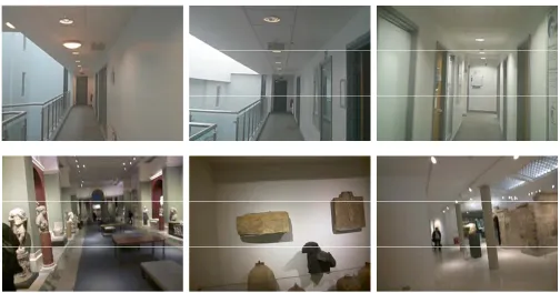
Fig. 13. Two different experiment sites. Top: the office building, where left two images are taken at two different floors. Bottom: the museum.

If no consecutive strong image matchings can be found, i.e.Lv keeps low, localisation failure is confirmed. This means the live images are very different from those in the experience Ep_{, i.e.} now the user is exploring a route that hasn’t been traversed before. On the other hand, if we directly observe low Lv sequences, our system also declare localisation failure since the current appearance of the environment is significantly different from the previous experiences. In both cases, we pause state estimation, and save the current sensor observations as a new experience

En (as discussed in Sec 2.2). When the system observes a sequence of consecutive strong image matchings, it believes that the user is back to the previous experience Ep, and reinstates the state estimation process. In this way, our system handles localisation failure gracefully, and continues to accumulate a more comprehensive representation of the workspace.

5

E

5.1 Experiment Setup

Sites and Participants: The proposed approach is evaluated in two different indoor settings: an office building and a museum. The office site is a four-storey building with similar layout and appearance at each floor (roughly 65×35m2_{), as show in the top} row of Fig. 13. Note that the left two images are taken at different locations across two floors. The museum site is much bigger in size (∼110×55m2), and has lots of open space and complex objects such as shelves and statues, as shown in the bottom row of Fig. 13). We recruited five participants of different genders, heights and ages, and asked them to walk normally in both sites. During the experiments, the participants wore smart glasses, and held mobile phones in their hands (cameras facing forward) while walking. In our experiments, the cameras of the glasses and mobile phones were facing towards the moving direction for most of the time. However, this is not a restriction of the system, since if the device orientation changes significantly, our system will create new experiences to capture the appearance of the environment from new angles, which can be used in subsequence localisation. The participants have repeated a set of trajectories for several times, where we randomly select a subset (across different users) to form experience graph, and use the rest for testing.

TABLE 1

Hardware specs and computational capability of different devices.

Device CPU RAM MFLOPS

Google Glass Dual core @ 1.0GHz 1GB 53.13 Nexus 4 Quad core @ 1.5GHz 2GB 137.21 HTC One M8 Quad core @ 2.3GHz 2GB 311.95 Nexus 6 Quad core @ 2.7GHz 3GB 606.29

1 2 3 4 5

0 .2 .4 .6 .8 1

Localisation Error(m)

Cumulative Probability

1 2 3 4 5

0 .2 .4 .6 .8 1

Localisation Error(m)

Cumulative Probability

(a) (b)

SVM FAB-MAP NaviGlass L-Learning

Google Glass Nexus 6

Fig. 14. (a) Error distribution of offline localisation. (b) Error distribution of online localisation on different devices.

computational power (see Table. 1), but as shown later in Sec. 5.2, the proposed approach is able to achieve significant performance gain on all of them. Our visual processing pipeline (for both front-end and back-end) is built with OpenCV 2.4.10, and uses SURF [12] to extract visual features.

Ground Truth:We use the Conditional Random Fields (CRFs) based map matching approach (in [6]) to generate ground truth. We assume the accurate metrical maps (i.e. floorplans) are avail-able, and at certain points of the trajectories, the true positions of the users can be inferred from the captured images (e.g. at turns, or when passing by a unique landmark). Those known positions are manually labelled and fed into the CRFs model as priors, which help the map matching process converge to the correct estimates. Competing Algorithms:We compare the proposed lifelong learn-ing approach (referred to as L-Learning hereafter) with the following three competing algorithms: 1) SVM, which is our implementation of the existing Travi-Navi [3] system. It uses pedestrian dead-reckoning (PDR) to estimate the displacement of the user, and the Bag-of-Words (BOW) model to represent images. Given a trajectory, the images captured at nearby locations (e.g. within 3-step range) are clustered into groups to train a linear Support Vector Machine (SVM). During localisation, the observed images are matched to the saved ones based on the trained SVM. 2) FAB-MAP, which also uses PDR to compute the inertial trajectories, but considers the more advanced FAB-MAP model [9] for image matching. Comparing to the above SVM algorithm, it takes the important correlations between the visual words into account, and evaluates the similarity between images with a graphical model. However it does not incorporate any optimisation of the visual processing pipeline: it uses the whole vocabulary and full images at the same scale. 3) our previous workNaviGlass[8], which uses a similar processing pipeline as FAB-MAP, but with a globally reduced visual vocabulary. Note that comparing to the proposed L-Learning approach, it doesn’t consider the optimal image scales/regions, nor the spacial variations in visual words: it just uses a smaller visual vocabulary throughout. To be fair, for all algorithms we use the same PDR implementation, SURF parameters, and state estimation algorithm as in Sec. 4.

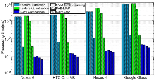
Nexus 6 HTC One M8 Nexus 4 Google Glass

101

102

103

104

Processing time(ms)

100

L-Learning SVM

FAB-MAP Feature Extraction

Feature Quantisation

BOW Comparison NaviGlass

Fig. 15. The running time of feature detection and quantisation per image for different devices. The proposed approach is up to 50×faster than the competing algorithms.

5.2 Experiment Results

Localisation Accuracy:The first set of experiments evaluate the localisation accuracy of the proposed (L-Learning) and competing (SVM, FAB-MAP and NaviGlass) algorithms given their different visual processing techniques. We first consider the ideal offline scenarios, where the mobile devices are allowed to process all of the captured images beforehand, and report user positions later. Fig. 14(a) shows the distribution of localisation errors in offline. We can see that the naive SVM has much larger errors comparing to FAB-MAP, NaviGlass and the proposed L-Learning, and the gap between the latter three algorithms is very small. This means although L-Learning only processes a tiny portion of information comparing to FAB-MAP and NaviGlass, it is able to achieve nearly the same accuracy. On the other hand, in online localisation scenarios, the accuracy of SVM, FAB-MAP and NaviGlass drops significantly, as shown in Fig. 14(b). This is because the expensive visual processing pipeline severely limits the image rate, e.g. on Nexus 6 it takes about 4s to process one 800×600 image and Google glasses need almost 20s to finish (see Fig. 15). Thus those algorithms can’t correct the fast growing drifts of PDR in time during online positioning. However, the proposed L-Learning algorithm does not suffer from such a problem since it is much more lightweight (<100ms on Nexus 6), and is able to localise in real-time with high accuracy (mean error 0.96m).

16 8 4 2 1 .5 .25

0 4 8 12

0 1 2

0 2 4 6 8 10 12

20 40

Localisat

ion

Error

(m)

Energy

C

onsumpt

ion

(W)

0 2 4 6 8 10 12

20 40

CPU

Load (%

)

Image Sampling Interval (s) Time (s)

(a) (b)

L-Learning Power NaviGlass Power

L-Learning Error NaviGlass Error

NaviGlass

L-Learning

Fig. 16. (a) Localisation accuracy and energy consumption under dif-ferent image sampling intervals. (b) Normalised CPU load of NaviGlass (top) and L-Learning (bottom) when sampling images every 4s.

TABLE 2

Estimated battery life (hours) of running NaviGlass and L-Learning.

Sampling Interval (s) 16 8 4 2

NaviGlass 6.9 6.6 6.3 5.2 L-Learning 7.5 7.3 7.0 6.3

Accuracy vs. Resource Consumption:The third set of experi-ments investigate the trade-off between localisation accuracy and resource consumption of the proposed system. Fig 16(a) shows the mean localisation error and the energy consumption of our system and the state-of-the-art NaviGlass when the image sampling in-terval varies from 16s to 0.25s. Note that here we only evaluate the systems on the Nexus 6 (with Qualcomm Trepn Profiler [15]), since on other devices NaviGlass takes too long to process images (see Fig. 15). As shown in Fig 16(a), NaviGlass is only able to process images every 2s, while the proposed L-Learning can process 4 images per second. In addition, for both approaches smaller image sampling intervals lead to lower localisation error, but also cause higher energy consumption. Table. 2 shows the estimated battery life of NaviGlass and the proposed L-Learning, which is evaluated by running the algorithms for one hour period, and then projecting the expected battery life based on the observed energy consumption. We repeat this procedure for five times and report the average. We see that for L-Learning, when capturing images at 1Hz, the positioning error has already dropped around 1m, while the gain in accuracy becomes marginal when the image sampling rate further increases. Finally, although the localisation error of NaviGlass is comparable to L-Learning, to process the same amount of images, L-Learning only consumes about half energy of NaviGlass. As a result, on Nexus 6 L-Learning can achieve up to 21% longer battery life than NaviGlass, as shown in Table. 2. This is because NaviGlass takes much longer time to process each image, where the CPU is constantly occupied, as shown in Fig. 16(b). Therefore, when energy is not an issue, only L-Learning has the option to sample denser images to improve accuracy: as in Fig. 16(a), comparing to the best performance produced by NaviGlass, L-Learning can further reduce the locali-sation error to about 1/3.

Impact of Key Word Discovery:This set of experiments evaluate the proposed key word discovery techniques. We keep images at the original scale without salient regions, but vary the size of the key word set, from 10% to the complete vocabulary. To exclude the impact of the inertial measurements, here we consider the image matching error, which is the mean distance between the locations of the matched images and the ground truth. Fig. 17(a) shows the image matching accuracy when using different amount of key

0 5 10 15

10 20 30 40 50 60 70 80 90 100 Amount of key words(%)

Mean image

matching

err

o

r(

m)

10 20 30 40 50 60 70 80 90 100 1

3 5 7 9

Amount of key words(%)

Feature

quan

tisatio

n

time (

s)

(a) (b)

Greedy Random

Google Glass Nexus 6

Fig. 17. (a) Mean image matching error, and (b) running time of feature quantisation per image when considering different amount of key words.

0 1 2 3 4 5 6 7 8m

0 10 20

0 1 2 3 4 5 6 7 8m

0 10 20

% %

Percentage

Percentage

Distance until recovery Distance before detecting lost

(a) (b)

Fig. 18. Distance travelled between (a) the actual deviation point and when detecting localisation failure, and (b) the actual return point and when successful localisation is resumed.

0 5 10 15

.1 .2 .3 .4 .5 .6 .7 .8 .9 1 Image scales

Mean image ma

tching

erro

r(m)

0 .2 .4 .6 .8 1

.1 .2 .3 .4 .5 .6 .7 .8 .9 1 Image scales

Sali

ent reg

ion ratio

w/o salient region(SR) with salient region(SR)

0

1 3 5 7 9

.1 .2 .3 .4 .5 .6 .7 .8 .9 1

Feature extraction time(s)

0

.1 .2 .3 .4 .5 .6 .7 .8 .9 1 1

3 5 7 9

Feature quan

tisation time(s)

(a) (b) (c) (d)

Glass w/o SR Glass with SR Nexus 6 w/o SR Nexus 6 with SR

Glass w/o SR Glass with SR Nexus 6 w/o SR Nexus 6 with SR

Image scales Image scales

Fig. 19. (a) Mean image matching error at different image scales, with/without salient region detection. (b) Relative sizes of the detected salient regions (percentage comparing to the full image) at different scales. (c) Running time of feature detection, and (d) quantisation at different image scales.

0 10 20 30 40 50

0 10 15 20 25 30

(b)

(b2) (b1) %

(a) (a1)

(a2)

Fig. 20. (a) The optimal percentage of key words (relative to the complete vocabulary), and (b) pixels (relative to the original image size) learned by the proposed algorithm across the visual experiences at the museum site.

smaller (<30% at scale 1). This is because higher scale images typically contain more detail, and thus features extracted from smaller salient regions are sufficient to achieve correct matching. Thirdly, using variable image scales has effect on the running time of both feature extraction and quantisation. As shown in Fig. 19(c) and (d), the feature extraction time increases quadratically with respect to image scales, but the growth of quantisation time slows down at higher scales. This is also expected because under the BOW model, the quantisation cost is proportional to the number of uniquewords, where higher scale images tend have a lot of repetitions of the same visual elements. Finally, using salient regions won’t be able to save much in feature quantisation (Fig. 19(d)), but could significantly reduce the feature extraction time, especially at high scales (Fig. 19(c)). This confirms that our salient region detection algorithm can effectively reduce the amount of pixels needed to be processed, while still keep most of the important visual elements appear in the images.

Spatial Variations:This experiment shows the spatial variations of the parameters learned by the proposed approach. Fig. 20(a) illustrates the sizes of optimal key word sets (percentage of the full vocabulary) across space, and Fig. 20(b) is the amount of pixels (percentage of all pixel in the original image) contained in the detected salient regions. Firstly, we see in most areas the learned parameters only contain a small portion of the original vocabulary or pixels, e.g. we only have to consider at most half of the whole vocabulary, while the average amount of pixels needed to be processed is roughly 10∼15% of the original image. However, we do observe clear spatial variations. For instance in image Fig. 20(a1), the scene is dominated by common visual elements, such as lights or door frames, and thus more words are required to distinguish it from the others within that area. On