warwick.ac.uk/lib-publications
Original citation:
Chistikov, Dmitry, Dimitrova, Rayna and Majumdar, Rupak. (2017) Approximate counting in
SMT and value estimation for probabilistic programs. ACTA Informatica .
Permanent WRAP URL:
http://wrap.warwick.ac.uk/89255
Copyright and reuse:
The Warwick Research Archive Portal (WRAP) makes this work by researchers of the
University of Warwick available open access under the following conditions. Copyright ©
and all moral rights to the version of the paper presented here belong to the individual
author(s) and/or other copyright owners. To the extent reasonable and practicable the
material made available in WRAP has been checked for eligibility before being made
available.
Copies of full items can be used for personal research or study, educational, or not-for profit
purposes without prior permission or charge. Provided that the authors, title and full
bibliographic details are credited, a hyperlink and/or URL is given for the original metadata
page and the content is not changed in any way.
Publisher’s statement:
The final publication is available at Springer via
http://dx.doi.org/10.1007/s00236-017-0297-2
A note on versions:
The version presented here may differ from the published version or, version of record, if
you wish to cite this item you are advised to consult the publisher’s version. Please see the
‘permanent WRAP url’ above for details on accessing the published version and note that
access may require a subscription.
(will be inserted by the editor)
Approximate Counting in SMT and
Value Estimation for Probabilistic Programs
Dmitry Chistikov · Rayna Dimitrova · Rupak Majumdar
Received: date / Accepted: date
Abstract #SMT, or model counting for logical theories, is a well-known hard problem that generalizes such tasks as counting the number of satisfying assignments to a Boolean for-mula and computing the volume of a polytope. In the realm of satisfiability modulo theories (SMT) there is a growing need for model counting solvers, coming from several application domains (quantitative information flow, static analysis of probabilistic programs). In this paper, we show a reduction from an approximate version of #SMT to SMT.
We focus on the theories of integer arithmetic and linear real arithmetic. We propose model counting algorithms that provide approximate solutions with formal bounds on the approximation error. They run in polynomial time and make a polynomial number of queries to the SMT solver for the underlying theory, exploiting “for free” the sophisticated heuris-tics implemented within modern SMT solvers. We have implemented the algorithms and used them to solve the value problem for a model of loop-free probabilistic programs with nondeterminism.
Keywords #SMT ·model counting·satisfiability modulo theory· #SAT·volume computation·approximation algorithms·probabilistic programming
1 Introduction
Satisfiability modulo theories (SMT) is a foundational problem in formal methods, and the research landscape is not only enjoying the success of existing SMT solvers, but also gen-erating demand for new features. In particular, there is a growing need formodel counting
solvers; for example, questions in quantitative information flow and in static analysis of probabilistic programs are naturally cast as instances of model counting problems for ap-propriate logical theories [24, 43, 52].
We define the #SMT problem that generalizes several model counting questions relative to logical theories, such as computing the number of satisfying assignments to a Boolean formula (#SAT) and computing the volume of a bounded polyhedron in a finite-dimensional real vector space. Specifically, to define model counting modulo ameasured theory, first suppose every variable in a logical formula comes with a domain which is also a measure
space. Assume that, for every logical formulaϕin the theory, the set of its modelsJϕKis
measurable with respect to the product measure; themodel counting (or#SMT)problem then asks, givenϕ, to compute the measure ofJϕK, called themodel countofϕ.
In our work we focus on the model counting problems for the theories of bounded integer arithmetic and linear real arithmetic. These problems are complete for the complexity class #P, so fast exact algorithms are unlikely to exist.
We extend to the realm of SMT the well-known hashing approach from the world of #SAT, which reducesapproximateversions of counting to decision problems. From a theo-retical perspective, we solve a model counting problem with a resource-bounded algorithm that has access to an oracle for the decision problem. From a practical perspective, we show how to use unmodified existing SMT solvers to obtain approximate solutions to model-counting problems. This reduces an approximate version of #SMT to SMT.
Specifically, for integer arithmetic (not necessarily linear), we give a randomized algo-rithm that approximates the model count of a given formulaϕ to within a multiplicative
factor(1+ε)for any givenε >0. The algorithm makesO(1
ε|ϕ|)SMT queries of size at
mostO(1 ε2|ϕ|
2)where|ϕ|is the size of
ϕ.
For linear real arithmetic, we give a randomized algorithm that approximates the model count with an additive errorγN, whereN is the volume of a box containing all models of the formula, and the coefficientγis part of the input. The number of steps of the algorithm
and the number of SMT queries (modulo the combined theory of integer and linear real arithmetic) are again polynomial.
As an application, we show how to solve the value problem (cf. [52]) for a model of loop-free probabilistic programs with nondeterminism.
Techniques
Approximation of #Pfunctions by randomized algorithms has a rich history in complexity theory [58, 62, 34, 33]. Jerrum, Valiant, and Vazirani [34] described a hashing-basedBPPNP procedure to approximately compute any #Pfunction, and noted that this procedure already appeared implicitly in previous papers by Sipser [54] and Stockmeyer [58]. The procedure works with encoded computations of a Turing machine and is thus unlikely to perform well in practice. Instead, we show a direct reduction from approximate model counting to SMT solving, which allows us to retain the structure of the original formula. An alternate ap-proach could eagerly encode #SMT problems into #SAT, but experience with SMT solvers suggests that a “lazy” approach may be preferable for some problems.
For the theory of linear real arithmetic, we also need an ingredient to handle continuous domains. Dyer and Frieze [19] suggested a discretization that introduces bounded additive error; this placed approximate volume computation for polytopes—or, in logical terms, ap-proximate model counting for quantifier-free linear real arithmetic—in #P. Motivated by the application in the analysis of probabilistic programs, we extend this technique to han-dle formulas with existentially quantified variables, while Dyer and Frieze only work with quantifier-free formulas. To this end, we prove a geometric result that bounds the effect of projections: this gives us an approximate model counting procedure for existentially quanti-fied linear arithmetic formulas. Note that applying quantifier elimination as a preprocessing step can make the resulting formula exponentially big; instead, our approach works directly on the original formula that contains existentially quantified variables.
suggests that simple randomized algorithms using off-the-shelf SMT solvers can be effective on small examples.
Counting in SMT
#SMT is a well-known hard problem whose instances have been studied before, e. g., in volume computation [19], in enumeration of lattice points in integer polyhedra [2], and as #SAT [28]. Indeed, very simple sub-problems, such as counting the number of satisfy-ing assignments of a Boolean formula or computsatisfy-ing the volume of a union of axis-parallel rectangles inRn(called Klee’s measure problem [37]) are already #P-hard (see Section 2
below).
Existing techniques for #SMT either incorporate model counting primitives into propo-sitional reasoning [44, 63, 5] or are based on enumerative combinatorics [40, 43, 24]. Typi-cally, exact algorithms [40, 44, 24] are exponential in the worst case, whereas approximate algorithms [43, 63] lack provable performance guarantees. In contrast to exact counting tech-niques, our procedure is easily implementable and uses “for free” the sophisticated heuris-tics built in off-the-shelf SMT solvers. Although the solutions it produces are not exact, they provably meet user-provided requirements on approximation quality. This is achieved by extending the hashing approach from SAT [27, 28, 10, 21] to the SMT context.
A famous result of Dyer, Frieze, and Kannan [20] states that the volume of a convex polyhedron can be approximated with a multiplicative error in probabilistic polynomial time (without the need for an SMT solver). In our application, analysis of probabilistic programs, we wish to compute the volume of a projection of a Boolean combination of polyhedra; in general, it is, of course, non-convex. Thus, we cannot apply the volume estimation algorithm of [20], so we turn to the “generic” approximation of #Pusing anNPoracle instead. Our #SMT procedure for linear real arithmetic allows an additive error in the approximation; it is known that the volume of a polytope does not always have a small exact representation as a rational number [41].
An alternative approach to approximate #SMT is to apply Monte Carlo methods for volume estimation. They can easily handle complicated measures for which there is limited symbolic reasoning available. Like the hashing technique, this approach is also exponential in the worst case [33]: suppose the volume in question, p, is very small and the required precision is a constant multiple ofp. In this case, Chernoff bound arguments would suggest the need forΩ(1p)samples; the hashing approach, in contrast, will perform well. So, while in “regular” settings (whenpis non-vanishing) the Monte Carlo approach performs better, “singular” settings (when pis close to zero) are better handled by the hashing approach. The two techniques, therefore, are complementary to each other (see the remark at the end of Subsection 5.5).
Related work
well. Ermon et al. also consider a weighted setting where the weights of satisfying assign-ments are given in a factorized form; for this setting, as a basic building block, they invoke an optimization solver ToulBar2 [1] to answer MAP (maximum a posteriori assignment) queries. More recently and concurrently with (the conference version of) our work, Belle, Van den Broeck, and Passerini [4] apply the techniques of Chakraborty et al. in the context of so-called weighted model integration. This is an instance of #SMT where the weights of the satisfying assignments (models) are computed in a more complicated fashion. Belle et al. adapt the procedure of Chakraborty et al., also using CryptoMiniSat, but additionally rely on the Z3 SMT solver to check candidate models against the theory constraints (real arithmetic in this case) encoded by the propositional variables, and use the LattE tool [40] for computing the volume of polyhedra.
We briefly review the problem settings of Ermon et al. [21] and Belle et al. [4, 5] in Section 2. In our work, the problem setting is more reminiscent of those in Chakraborty et al. [10] and Ermon et al. [21], and the hashing approach itself is the same as the one de-scribed, e.g., in [10] for the #SAT case. We lift this idea to the SMT world, in particular for the cases of bounded integer arithmetic and linear real arithmetic with existential quantifi-cation. Our implementation is a proof of concept for the extension, to SMT, of the hashing approach to approximate model counting. While we discuss some preliminary experiments in Section 6, a scalable implementation and extensive empirical evaluation are beyond the scope of this paper. We now outline some challenges towards a scalable tool for #SMT.
From an implementation perspective, bounded integer arithmetic can be reduced to the Boolean case, which is readily handled by approximate #SAT tools such asApproxMC[10]. Modern SMT solvers such as Z3 [17] contain conversion and preprocessing heuristics to bit-blast arithmetic formulas. Our approach, on the other hand, handles bounded integer arith-metic formulas directly, relying on the SMT solver for performing word-level reasoning. As in SMT solving, the relative performance of the two techniques (direct theory reasoning vs. bitblasting) is likely to depend on the considered benchmarks, and choosing between them in a practical tool remains an open problem.
Our use of hashing introduces many Boolean XOR constraints. Modern SAT solvers perform poorly on XOR constraints, unless they implement specialized heuristics (see, e.g., the CryptoMiniSat solver [55]). Our implementation currently uses an unmodified theory solver with an additional pre-processor that solves the system of XOR equations (see Sub-section 5.6). A better implementation would replace the “usual” SAT solver within the SMT solver to one that has special heuristics for XOR constraints, e.g., those implemented in CryptoMiniSat. An open question is whether there is a different family of hash functions that combines well with theory reasoning. A step in this direction was taken by Chakraborty et al. in their recent work [11], where they use word-level hashing functions to enable better us-age of the power of modern SMT solvers. Chakraborty et al. show, empirically, that on a large number of benchmarks word-level reasoning leads to improved performance com-pared to the bit-level XOR reasoning. However, they also establish that these word-level hash functions do not help for formulas involving word-level multiplication—and, in fact, the XOR-based approach performs better on several such benchmarks [11].
Contributions
We extend, from SAT to SMT, the hashing approach to approximate model counting:
2. For the theory of bounded integer arithmetic, we provide a direct reduction (Theorem 1 in Section 2) from approximate counting to SMT.
3. For the theory of bounded linear real arithmetic, we give a technical construction (Lemma 2 in Subsection 3.3) that lets us extend the results of Dyer and Frieze to the case where the polyhedral set is given as a projection of a Boolean combination of polytopes; this leads to an approximate model counting procedure for this theory (Theorem 2 in Section 2). 4. As an application, we show that the value problem for small loop-free probabilistic
programs with nondeterminism reduces to #SMT (Section 5).
The conference version of this paper appeared as [13].
2 The #SMT Problem
We present a framework for a uniform treatment of model counting both in discrete theories like SAT (where it is literally counting models) and in linear real arithmetic (where it is really volume computation for polyhedra). We then introduce the notion of approximation and give an algorithm for approximate model counting by reduction to SMT.
Preliminaries: Counting Problems and#P
A relationR⊆Σ∗×Σ∗ is ap-relation if (1) there exists a polynomial p(n)such that if
(x,y)∈Rthen|y|=p(|x|)and (2) the predicate(x,y)∈Rcan be checked in deterministic polynomial time in the size ofx. Intuitively, a p-relation relates inputsxto solutionsy. It is easy to see that a decision problemLbelongs toNPif there is a p-relationRsuch that
L={x| ∃y.R(x,y)}.
Acounting problemis a function that mapsΣ∗ toN. A counting problem f:Σ∗→N
belongs to the class #Pif there exists a p-relationRsuch that f(x) =|{y|R(x,y)}|, i. e., the class #Pconsists of functions that count the number of solutions to a p-relation [61].
Completenessin #Pis with respect to Turing reductions; the same term is also (ab)used to encompass problems that reduce to a fixed number of queries to a #Pfunction (see, e. g., [19]).
#SAT is an example of a #P-complete problem: it asks for the number of satisfying assignments to a Boolean formula in conjunctive normal form (CNF) [61]. Remarkably, #Pcharacterizes the computational complexity not only of “discrete” problems, but also of problems involving real-valued variables: approximate volume computation (with additive error) for bounded rational polyhedra inRkis #P-complete [19].
Measured Theories and#SMT
We will now define the notion of model counting that generalizes #SAT and volume com-putation for polyhedra. SupposeT is a logical theory. Letϕ(x)be a formula in this theory with free first-order variablesx= (x1, . . . ,xk). Assume thatT comes with a fixed interpre-tation which specifies domains of the variables, denotedD1, . . . ,Dk, and assigns a meaning to predicates and function symbols in the signature ofT. Then a tuplea= (a1, . . . ,ak)∈
D1×. . .×Dkis called amodelofϕif the sentenceϕ(a1, . . . ,ak)holds, i. e., ifa|=T ϕ(x). We denote the set of all models of a formulaϕ(x)byJϕK; thesatisfiability problemforT
Consider the special cases of #SAT and volume computation for polyhedra; the corre-sponding satisfiability problems are SAT and linear programming. For #SAT, atomic pred-icates are of the formxi=b, forb∈ {0,1}, the domainDiof eachxiis{0,1}, and formulas are propositional formulas in conjunctive normal form. For volume computation, atomic predicates are of the formc1x1+. . .+ckxk≤d, forc1, . . . ,ck,d∈R, the domainDiof each
xiisR, and formulas are conjunctions of atomic predicates. SetsJϕKin these cases are the
set of satisfying assignments and the polyhedron itself, respectively.
Suppose the domainsD1, . . . ,Dkgiven by the fixed interpretation are measure spaces: eachDiis associated with aσ-algebraFi⊆2Diand a measureµi:Fi→R. This means, by
definition, thatFiandµisatisfy the following properties:Ficontains /0 and is closed under complement and countable unions, andµiis non-negative, assigns 0 to /0, and isσ-additive.1
In our special cases, these spaces are as follows. For #SAT, eachFi is the set of all subsets ofDi={0,1}, andµi(A)is simply the number of elements inA. For volume com-putation, eachFiis the set of all Borel subsets ofDi=R, andµiis the Lebesgue measure. Assume that each measureµiisσ-finite, that is, the domainDiis a countable union of measurable sets (i. e., of elements ofFi, and so with finite measure associated with them). This condition, which holds for both special cases, implies that the Cartesian productD1×
. . .×Dkis measurable with respect to a uniqueproduct measureµ, defined as follows. A set
A⊆D1×. . .×Dkismeasurable(that is,µassigns a value toA) if and only ifAis an element of the smallestσ-algebra that contains all sets of the formA1×. . .×Ak, withAi∈Fifor all
i. For all such sets, it holds thatµ(A1×. . .×Ak) =µ1(A1). . .µk(Ak).
In our special cases, the product measureµ(A)of a setAis the number of elements in
A⊆ {0,1}kand the volume ofA⊆
Rk, respectively.
We say that the theoryT ismeasuredif for every formulaϕ(x)inT with free (first-order) variablesx= (x1, . . . ,xk)the setJϕKis measurable. We define themodel countof a
formulaϕasmc(ϕ) =µ(JϕK). Naturally, if the measures in a measured theory can assume
non-integer values, the model count of a formula is not necessarily an integer. With every measured theory we associate amodel counting problem, denoted #SMT[T]: the input is a logical formulaϕ(x)inT, and the goal is to compute the valuemc(ϕ).
The #SAT and volume computation problems are just special cases as intended, since
mc(ϕ)is equal to the number of satisfying assignments of a Boolean formula and to the volume of a polyhedron, respectively.
Note that one can alternatively restrict the theory to a fixed number of variables k, i.e., tox= (x1, . . . ,xk), where x∈D1×. . .×Dk, and introduce a measure µ directly on
D1×. . .×Dk; that is,µwill not be a product measure. Such measures arise, for instance,
whenµcomes in a factorized form where factors span non-singleton subsets of{x1, . . . ,xk}. A toy example, with k=3, might have µ induced by the probability density function Z·f1(x1,x2)·f2(x2,x3), where f1 and f2 are non-negative and absolutely continuous, and the normalization constantZ(sometimes calledthe partition function) is chosen in such a way thatµ(D1×D2×D3) =1. Note that computingZ, given f1and f2, is itself a #SMT-(i.e., model counting) question: the associated theory has measure ¯µinduced byf1·f2, and the goal is to computemc(true), where we assume thattrueis a formula in the theory with
JtrueK=D1×D2×D3. (Much more sophisticated) problems of this form arise in machine
learning and have been studied, e.g., by Ermon et al. [21].
Remark A different stance on model counting questions, under the name of weighted model integration (for real arithmetic), was recently suggested by Belle, Passerini, and Van den
1 The reader is referred to standard textbooks on probability and/or measure theory for further background;
Broeck [5]. Their problem setting starts with a tuple of real-valued (theory) variablesx=
(x1, . . . ,xk)and a logical formulaϕoverxand over standalone propositional variables,p=
(p1, . . . ,ps). All theory atoms in the formula are also abstracted as (different) propositional variables,q= (q1, . . . ,qt). All literalsl of propositional variables p,qare annotated with weight functions fl(x), which (can) depend on x. Take any total assignment to p,qthat satisfies the propositional abstraction ofϕand letLbe the set of all satisfied literals. The weight of this assignment top,qis the integralR
∏l∈Lfl(x)dxtaken over the area restricted in Rk by the conjunction of atoms that are associated with literals l∈L. The weighted
model integral ofϕis then the sum of weights of all assignments (top,q) that satisfy the propositional abstraction ofϕ.
We discuss several other model counting problems in the following subsection.
Approximate Model Counting
We now introduceapproximate#SMT and show how approximate #SMT reduces to SMT. We need some standard definitions. For our purposes, arandomized algorithmis an algo-rithm that uses internal coin-tossing. We always assume, whenever we use the term, that, for each possible inputxtoA, the overall probability, over the internal coin tossesr, that A outputs a wrong answer is at most 1/4. (This error probability 1/4 can be reduced to any smallerα>0, by taking the median acrossO(logα−1)independent runs ofA.)
We say that a randomized algorithmA approximatesa real-valued functional problem C:Σ∗→Rwith an additive errorifA takes as input anx∈Σ∗and a rational numberγ>0
and produces an outputA(x,γ)such that
Pr|A(x,γ)−C(x)| ≤γU(x)≥3/4,
whereU :Σ∗→Ris some specific and efficiently computable upper bound on the absolute value ofC(x), i. e.,|C(x)| ≤U(x), that comes with the problemC. Similarly,A approx-imatesa (possibly real-valued) functional problemC:Σ∗→Rwith a multiplicative error
ifA takes as input anx∈Σ∗and a rational numberε>0 and produces an outputA(x,ε)
such that
Pr(1+ε)−1C(x)≤A(x,ε)≤(1+ε)C(x) ≥3/4.
The computation time is usually considered relative to|x|+γ−1 or|x|+ε−1, respectively
(note the inverse of the admissible error). Polynomial-time algorithms that achieve approx-imations with a multiplicative error are also known as fully polynomial-time randomized approximation schemes (FPRAS) [34].
Algorithms can be equipped withoraclessolving auxiliary problems, with the intuition that an external solver (say, for SAT) is invoked. In theoretical considerations, the definition of the running time of such an algorithm takes into account the preparation ofqueriesto the oracle (just as any other computation), but not the answer to a query—it is returned within a single time step. Oracles may be defined as solving some specific problems (say, SAT) as well as any problems from a class (say, fromNP). The following result is well-known.
In the rest of this section, we present our results on the complexity of model counting problems, #SMT[T], for measured theories. For these problems, we develop randomized polynomial-time approximation algorithms equipped with oracles, in the flavour of Propo-sition 1. We describe the proof ideas in Section 3, and details are provided in Appendix. We formally relate model counting and the value problem for probabilistic programs in Sec-tion 5; in the implementaSec-tion, we substitute an appropriate solver for the theory oracle. We illustrate our approach on an example in Section 4.
Integer arithmetic. ByIAwe denote theboundedversion of integer arithmetic: each free variablexiof a formulaϕ(x1, . . . ,xk)comes with a bounded domainDi= [ai,bi]⊆Z, where ai,bi∈Z. We use the counting measure| · |:A⊆Z7→ |A|, so the model countmc(ϕ)of
a formulaϕ is the number of its models. In the formulas, we allow existential (but not universal) quantifiers at the top level. The model counting problem forIAis #P-complete.
Example 1 Consider the formula
ϕ(x) =∃y∈[1,10].(x≥1)∧(x≤10)∧(2x+y≤6)
=∃y.(y≥1)∧(y≤10)∧(x≥1)∧(x≤10)∧(2x+y≤6)
in the measured theoryIA. This formula has one free variablexand one existentially quan-tified variabley, let’s say both with domain[0,10]. It is easy to see that there exist only two values ofx,x≥1, for which there exists ay≥1 with 2x+y≤6: these are the integers 1
and 2. Hence,mc(ϕ) =2. ut
Theorem 1 The model counting problem forIAcan be approximated with a multiplicative error by a polynomial-time randomized algorithm that has oracle access to satisfiability of formulas inIA.
Linear real arithmetic. ByRAwe denote theboundedversion of linear real arithmetic, with possible existential (but not universal) quantifiers at the top level. Each free variablexiof a formulaϕ(x1, . . . ,xk)comes with a bounded domainDi= [ai,bi]⊆R, whereai,bi∈R.
The associated measure is the standard Lebesgue measure, and the model countmc(ϕ)of a formulaϕ is the volume of its set of models. (Since we consider linear constraints, any
quantifier-free formula defines a finite union of polytopes. It is an easy geometric fact that its projection on a set of variables will again be a finite union of bounded polytopes. Thus, existential quantification involves only finite unions.)
Example 2 Consider the same formula
ϕ(x) =∃y∈[1,10].(x≥1)∧(x≤10)∧(2x+y≤6)
=∃y.(y≥1)∧(y≤10)∧(x≥1)∧(x≤10)∧(2x+y≤6),
this time in the measured theoryRA, wherex∈Randy∈R. Note that nowϕ(x)is equivalent to(x≥1)∧(x≤2.5), and thusmc(ϕ) =1.5: this is the length of the line segment defined
by this constraint. ut
3 Proof Techniques
In this section we explain the techniques behind Theorems 1 and 2. The detailed analysis can be found in Appendix.
3.1 Intuition: Hashing-based approximate counting
Let us first explain how the hashing-based approach to approximate counting works. In this subsection we will describe the intuition behind the approach on an abstract level using very simple examples and without referring to any implementation issues. We will later (Subsections 3.2 and 3.3) present the approach in more generality and explain how it can be implemented in practice.
The core of the hashing approach is the following high-level observation (see, e.g., Jer-rum et al. [34], and historical notes in the introduction above). LetHmbe a family of hash functions of the formh:D→ {0,1}mwith properties to be fixed below. Intuitively, one ex-pects that, for each elementa∈D, if a functionhis picked at random fromHm, then the imageh(a)attains all values from{0,1}mwith equal probabilities. For example, the proba-bility thath(a) =0mshould equal 1/2m. Moreover, this behaviour should, in a way, extend from single elementsa∈Dto sets: with high probability, the number of elements of a set
S⊆Dthat satisfyh(a) =0mshould be close to|S|/2m. Since this number is, in fact, always integral, one can expect it to be positive if|S| 2mand equal to zero if|S| 2m. Obviously, for each setSthere will be individual functionsh∈Hmviolating these inequalities, but for the majority of functionsh∈Hmthese inequalities will hold.
Now the idea is to use this observation for estimating the cardinality of a set that is not given to us explicitly. In the scenario we are interested in, the setSwill be the set of all models of a given formula. More formally, consider a formulaϕ(x)in some measured theory with one free variable. For simplicity, suppose the theory isIA, integer arithmetic with a bounded domainD= [0,M], where the measure of a setA⊆Dis simply the cardinality of
A. Denote bySthe set of all models of the formulaϕ(x), i.e.,S=JϕK. If, as above, the hash
functionh:D→ {0,1}mis chosen at random from an appropriate familyH
m, then with high probability the formulaϕ(x)∧(h(x) =0m)is satisfiable ifmc(ϕ)2mand unsatisfiable if
mc(ϕ)2m.
Example 3 Supposeϕ(x)is the formulax=42, and the domain of the variablexis D= [0,255]. The setS=JϕKis a singleton:S={42}. SinceS6=/0, that is, the formulaϕ(x)is
satisfiable, we start the process described above.
We setm=1 at first and draw a hash functionh1:D→ {0,1}at random from the setH1. Let us omit the description of the setH1; suppose the hash function that we draw happens to beh1(x) =xmod 2. We now check satisfiability of the formulaϕ(x)∧(xmod 2=0), which is equivalent to(x=42)∧(xmod 2=0). Asx=42 is a model of this formula, we proceed tom=2. Now we need to draw a hash function fromH2. Suppose it has the form
h2(x) =bx/64c where the result is interpreted as an element of{0,1}2 in a natural way. Sinceb42/64c=0, the formula (x=42)∧(h2(x) = (0,0))is satisfiable. Once we have determined this, we proceed tom=3. Here we need to draw a hash function at random from the setH3; suppose we drawh3(x) = (h31,h32,h33)whereh31= (x+1)mod 2; then, regardless of howh32andh33are defined, the formula(x=42)∧(h3(x) = (0,0,0))will be unsatisfiable. Therefore, our process will terminate atm=3.
What will be the outcome of the process? The exact answer is tightly related to the properties of the families of the hash functionsHm. More precisely, we asserted previously that with high probability the formulaϕ(x)∧(h(x) =0m)whereh∈Hm is satisfiable if
mc(ϕ)2mand unsatisfiable ifmc(ϕ)2m. The precise meaning ofandwill, in fact, influence the final estimate ofmc(ϕ). From the fact that in our run the process termi-nates atm=3 we can draw the conclusion that (with high probability)mc(ϕ)belongs to the interval[u∗2m,u∗2m] = [8u∗,8u∗]whereu∗andu∗are positive constants that do not depend
on the formulaϕand form a part of the description of our algorithm. One can imagine, for instance, thatu∗=1/2 andu∗=1; in our case this will give us the interval[4,8]. (The actual
formulas definingu∗andu∗can be found in Subsection A.2.) Of course, in our case this
an-swer will not be very satisfactory, because the correct value ofmc(ϕ)is 1. If, however, we compute the probability of such an outcome, i.e., the probability that the process will only terminate atm≥3 on inputϕ, we will see that this is a moderately rare event. If each bit of all hash functions fromHmis chosen independently (imagine, for example, that pickingh fromHmcorresponds to picking the values of eachh(x)independently and uniformly—this corresponds to the “ideal” hashing), then this probability will be 1/8. In comparison, with probability 1/2 the process will stop atm=1, which corresponds to the interval[1/2,1]— and this interval contains the correct value. Standard error reduction techniques will help us amplify the probability of such successful outcomes, thus making it very likely (according to our choice ofα) that the guessed interval will contain the correct value ofmc(ϕ). In
general, with high probability, the higher the values ofmthat the process attains, the larger
the estimate ofmc(ϕ). ut
3.2 Approximate discrete model counting
We now explain the idea behind Theorem 1 in more detail, zooming in on some aspects that we only sketched previously. Letϕ(x)be an input formula inIAand letx= (x1, . . . ,xk)be the free variables ofϕ. SupposeMis a big enough integer such that all models ofϕhave
components not exceedingM, i. e.,JϕK⊆[0,M]
k.
Our approach to approximatingmc(ϕ) =|JϕK|works as follows. Suppose our goal is
to find a valuevsuch thatv≤mc(ϕ)≤2v, and we have an oracleE, for “Estimate”, an-swering questions of the formmc(ϕ)≥?N. Then it is sufficient to make such queries toE
forN=Nm=2m,m=0, . . . ,klog(M+1), and the overall algorithm design is reduced to
Algorithm 1:Approximate model counting forIA
Input: formulaϕ(x)inIA Output: valuev∈R
Parameters: ε∈(0,1),/* approximation factor */ α∈(0,1),/* error probability */
a∈N/* enumeration limit for SMT solver */
Compute valuesm∗,q,p,rbased on parameters (see text);
1 if(e:=SMT(ϕ,p+1))≤pthen returne;
2 ψ(x,x0) =ϕ(x)∧t(x,x0);
3 ψq(x,x0) =ψ(x1,x01)∧ψ(x2,x02)∧. . .∧ψ(xq,x0q);
4 k0:=number of bits inx0; 5 form=1, . . . ,m∗do
6 c:=0;/* majority vote counter */ 7 forj=1, . . . ,rdo
8 ifE(ψq,k0,m,a)thenc:=c+1
9 ifc≤r/2then break;
10 return q √
a·2m−0.5
As we already know, such an implementation can be done with the help ofhashing. Suppose that a hash functionh, taken at random from some familyH, maps elements of
[0,M]kto{0,1}m. If the familyH is chosen appropriately, then each potential modelw is mapped byh to, say, 0m with probability 2−m; moreover, one should expect that any setS⊆[0,M]kof sizedhas roughly 2−m·delements inh−1(0m) ={w∈[0,M]k|h(w) =
0m}. In other words, if|S| ≥2m, thenS∩h−1(0m)is non-empty with high probability, and if|S| 2m, thenS∩h−1(0m)is empty with high probability. So—rephrasing slightly the observations outlined above—our task is reduced to distinguishing between empty and non-empty sets. This, in turn, is a satisfiability question and, as such, can be entrusted to theIA
solver. As a result, we reduced the approximation of the model count ofϕto a series of satisfiability questions inIA.
Our algorithm posts these questions as SMT queries of the form
ϕ(x)∧t(x,x0)∧(h0(x0) =0m), (1)
wherexandx0 are tuples of integer variables, each component ofx0 is either 0 or 1, the formulat(x,x0)says thatx0is binary encoding ofx, and theIAformulah0(x0) =0mencodes the computation of the hash functionhon inputx.
Algorithm 2:Satisfiability “oracle”E
Input: formulaψq(x,x0)inIA;k0,m,a∈N
Output:trueorfalse 1 h0:=PICK-HASH(k0,m);
2 ψh0(x,x0) =ψq(x,x0)∧(h0(x0) =0m);
3 return(SMT(ψh0,a)≥a)/* check if ψh0 has at least a models */
Algorithm 1 is the basis of our implementation. It returns a valuevthat satisfies the in-equalities(1+ε)−1mc(ϕ)≤v≤(1+ε)mc(ϕ)with probability at least 1−α. Algorithm 1
given as Algorithm 2 asks the SMT solver forIAto produceamodels (for a positive integer parametera) to formulas of the form (1) by calling the procedure SMT.
To achieve the required precision with the desired probability, the algorithm constructs a conjunction ofqcopies of the formula (over disjoint sets of variables), where the number of copiesqis defined2as
q=l1+4 log( √
a+1+1)−2 loga
2 log(1+ε)
m ;
we refer the reader to Subsection A.2 for a detailed description. This results in a formula withk0=qkdlog(M+1)e=O(|ϕ|/ε)binary variables, where|ϕ|denotes the size of the original formulaϕ. Then, in lines 5–9, Algorithm 1 performs for each dimension of the
hash function in the range{1, . . . ,m∗}a majority vote overrcalls to the procedureE, where the values ofm∗andrare computed as follows:
m∗=bk0−2 log(√a+1+1)c, r=
8·ln
1
α· bk
0−2 log(√a+1+1)c
.
For a formal derivation of these values, see Subsection A.3.
In a practical implementation, early termination of the majority-vote loop is possible as soon as the number of positive answers given byE exceedsr/2.
For formulasϕwith up top=d(√a+1−1)2/qemodels, Algorithm 1 returns the ex-act model countmc(ϕ)(line 1 in Algorithm 1) computed by the procedure SMT, which repeatedly calls the solver, counting the number of models up top+1.
The values of m∗,q,p, andrused in Algorithm 1, as well as the choice of the return valuev= q
√
a·2m−0.5, guarantee its correctness and are formally derived in Appendix A. For a fixed approximation factorεthe numberqof copies depends only on the parame-tera. More precisely, the larger the parameterais, the fewer copiesqare necessary. While, in general, smaller values forqresult in fewer variables in the queries to the SMT solver, the number of queries at each step of the loop in Algorithm 1 increases witha, albeit not drastically. One possible heuristic for balancing this trade-off is choosing asathe smallest value after which the value forqstabilizes. We have observed empirically that applying this heuristic leads to good performance, and have used it to select the values forafor the experiments on which we report in Section 5.6.
The family of hash functionsH used byPICK-HASHin Algorithm 2 needs to satisfy the condition of pairwise independence: for any two distinct vectorsx1,x2∈[0,M]k and any two stringsw1,w2∈ {0,1}m, the probability that a random functionh∈H satisfies
h(x1) =w1 andh(x2) =w2 is equal to 1/22m. The condition of pairwise independence is used by Algorithm 1 via the following proposition, known as (a simple form of) theLeftover Hash Lemma. It was originally proved by Impagliazzo, Levin, and Luby [32], and here we use a formulation due to Trevisan [59].
Lemma 1 LetH be a family of pairwise independent hash functions h:{0,1}n→ {0,1}m.
Let S⊆ {0,1}nbe such that|S| ≥4/ρ2·2m. For h∈H, let
ξ be the cardinality of the set {w∈S:h(w) =0m}. Then
Pr
ξ−|S|
2m
≥ρ·|S|
2m
≤1
4.
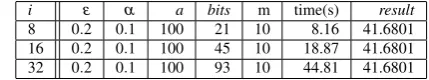
Table 1 Input and runtime parameters
i ε α a bits m time(s) result
8 0.2 0.1 100 21 10 8.16 41.6801 16 0.2 0.1 100 45 10 18.87 41.6801 32 0.2 0.1 100 93 10 44.81 41.6801
Legend:
ε: parameter in the multiplicative approximation factor(1+ε), α: maximum error probability,
a: the SMT enumeration threshold (number of models the SMT solver checks for),
bits: number of binary variables in the formula given to the solver,
m: maximal hash size,
result: approximate model count.
There are several constructions for pairwise independent hash functions; we employ a commonly used family, that of random XOR constraints [62, 3, 28, 9]. Givenk0andm, the family contains (in binary encoding) all functionsh0= (h01, . . . ,h0m):{0,1}k0→ {0,1}mwith
h0i(x1. . . ,xk0) =ai,0+∑k 0
j=1ai,jxj, whereai,j∈ {0,1}for alliand+is the XOR operator (ad-dition in GF(2)). By randomly choosing the coefficientsai,jwe get a random hash function from this family. The size of each query is thus bounded byO(k02) =O(1
ε2|ϕ|
2), where|
ϕ|
is again the size of the original formulaϕ, and there will be at mostm∗+1≤k0+O(1) = O(1ε|ϕ|)queries in total.
Example 4 Consider the formulaϕ(x) = (x≤42), where the integer variablexranges over the setsMi= [1,2i−1−1], fori∈ {8,16,32}. The model countmc(ϕ) =42 is small, while the size of the variable domain changes withiand fori=32 is quite significant. Table 1 illustrates the performance of our approximate counting algorithm on inputϕfor this set
of values of i. The parameterε in the multiplicative approximation factor (1+ε)is set
to 0.2, and the maximum error probabilityαis set to 0.1. We report the number of Boolean
variables in the formula given to the solver (after making the respective number of copies), and the running time in seconds. The table shows that the running time, as well as the number of calls to the SMT solver, are small, which reflects the small model count (the main loop of Algorithm 1 terminates early). As the size of the domain increases, the size of the SMT queries also increases, which, however, leads to only a moderate increase in the
overall running time. ut
Note that the entire argument remains valid even ifϕhas existentially quantified
vari-ables: queries (1) retain them as is. The prefix of existential quantifiers could simply be dropped from (1), as searching for models of quantifier-free formulas already captures ex-istential quantification. It is important, though, that the model enumeration done by the procedure SMT in Algorithms 1 and 2 only count distinct assignments to thefreevariables ofϕandψh0respectively.
3.3 Approximate continuous model counting
same domain. SupposeJϕK⊆[0,M]
kand fix some
γ, with the prospect of finding a valuev
that is at mostε=γMkaway frommc(ϕ)(we takeMkas the value of the upper boundU in the definition of additive approximation). We show below how to reduce this task of approx-imate continuous model counting to additive approximation of a model counting problem for a formula with a discrete set of possible models, which, in turn, will be reduced to that of multiplicative approximation.
We first show how to reduce our continuous problem to a discrete one. Divide the cube[0,M]kintosk small cubes with sideδ each,δ =M/s. For everyy= (y1, . . . ,yk)∈
{0,1, . . . ,s−1}k, set
ψ0(y) =1 if at least one point of the cubeC(y) ={yjδ ≤xj≤(yj+ 1)δ,1≤j≤k}satisfiesϕ; that is, ifC(y)∩JϕK6=/0.
Imagine that we have a formula ψ such thatψ(y) =ψ0(y) for all y∈ {0,1, . . . ,s−
1}k, and let
ψbe written in a theory with a uniform measure that assigns “weight”M/sto each pointyj∈ {0,1, . . . ,s−1}; one can think of these weights as coefficients in numerical integration. From the technique of Dyer and Frieze [19, Theorem 2] it follows that for a quantifier-freeϕand an appropriate value ofsthe inequality|mc(ψ)−mc(ϕ)| ≤ε/2 holds.
Indeed, Dyer and Frieze prove a statement of this form in the context of volume compu-tation of a polyhedron, defined by a system of inequalitiesAx≤b. However, they actually show a stronger statement: given a collection ofmhyperplanes inRkand a set[0,M]k, an
ap-propriate setting ofswill ensure that out ofskcubes with sideδ=M/sonly a small number
Jwill becut, i. e., intersected by some hyperplane. More precisely, ifs=
mk2Mk/(ε/2) , then this numberJ will satisfy the inequalityδk·J≤ε/2. Thus, the total volume of cut cubes is at mostε/2, and so, in our terms, we have|mc(ψ)−mc(ϕ)| ≤ε/2 as desired.
However, in our case the formulaϕneed not be quantifier-free and may contain
exis-tential quantifiers at the top level. Ifϕ(x) =∃u.Φ(x,u)whereΦis quantifier-free, then the
constraints that can “cut” thex-cubes are not necessarily inequalities fromΦ. These con-straints can rather arise from projections of concon-straints on variablesxand, what makes the problem more difficult, their combinations. However, we are able to prove the following statement:
Lemma 2 The numberJ of points y¯ ∈ {0,1, . . . ,s−1}kfor which cubes C(y)are cut satisfies ¯
δk·J¯≤ε/2ifδ¯=M/s, where¯ s¯=2m+2kk2Mk/(ε/2)=2m+2kk2/(γ/2)and m is the number of atomic predicates inΦ.
Proof Observe that a cubeC(y)is cut if and only if it is intersected by a hyperplane de-fined by some predicate in variablesx. Such a predicate does not necessarily come from the formulaΦitself, but can arise when a polytope in variables(x,u)is projected to the space associated with variables x. Put differently, each cut cubeC(y)has some d-dimensional face with 0≤d≤k−1 that “cuts” it; this face is an intersection ofC(y)with some affine subspaceπin variablesx.
Consider this subspaceπ. It can be, first, the projection of a hyperplane defined in
vari-ables(x,u)by an atomic predicate inΦor, second, the projection of an intersection of several
such hyperplanes. Now note that each predicate in(x,u)defines exactly one hyperplane; an intersection of hyperplanes in(x,u)projects to some specific affine subspace in variablesx. Therefore, each “cutting” affine subspaceπis associated with a distinct subset of atomic predicates inΦ, where, since the domain is bounded, we count in constraints 0≤xj≤Mas well. This gives us at most 2m+2kcutting subspaces, so it remains to apply the result of Dyer
and Frieze withm=2m+2k. ut
A consequence of the lemma is that the choice of the number ¯sensures that the formula
|mc(ψ)−mc(ϕ)| ≤ε/2. Here we associate the domain of each free variableyj∈ {0,1, . . . ,s¯− 1}with the uniform measureµj(v) =M/s¯. Note that the value of ¯schosen in Lemma 2 will still keep the number of steps of our algorithm polynomial in the size of the input, because the number of bits needed to store the integer index along each axis isdlog(s¯+1)eand not
¯
sitself.
As a result, it remains to approximatemc(ψ)with additive error of at mostε0=ε/2= γMk/2, which can be done by invoking the procedure from Theorem 1 that delivers approx-imation with multiplicative errorβ=ε0/Mk=γ/2.
4 A Fully Worked-Out Example
We now show how our approach to #SMT, developed in Sections 2 and 3 above, works on a specific example, coming from the value problem forprobabilistic programs. Probabilistic programs are a means of describing probability distributions; the model we use combines probabilistic assignments and nondeterministic choice, making programs more expressive, but analysis problems more difficult.
For this section we choose a relatively high level of presentation in order to convey the main ideas in a more understandable way; a formal treatment follows in Section 5, where we discuss (our model of) probabilistic programs and their analysis in detail.
The Monty Hall problem[53, 50]
We describe our approach using as an example the following classic problem from probabil-ity theory. Imagine a television game show with two characters: the player and the host. The player is facing three doors, numbered 1, 2, and 3; behind one of these there is a car, and behind the other two there are goats. The player initially picks one of the doors, say doori, but does not open it. The host, who knows the position of the car, then opens another door, say door jwith j6=i, and shows a goat behind it. The player then gets to open one of the remaining doors. There are two available strategies:staywith the original choice, doori, or
switchto the remaining alternative, doork6∈ {i,j}. The Monty Hall problem asks, which strategy is better? It is widely known that, in the standard probabilistic setting of the prob-lem, the switching strategy is the better one: it has payoff 2/3, i. e., it chooses the door with the car with probability 2/3; the staying strategy has payoff of only 1/3.
Modeling with a probabilistic program
We model the setting of the Monty Hall problem with the probabilistic program in Proce-dure 3: “Switch” strategy in Monty Hall problem, which implements the “switch” strategy. In this problem, there are several kinds of uncertainty and choice, so we briefly explain how they are expressed with the features of our programming model.
First, there is uncertainty in what door hides the car and what door the player initially picks. It is standard to model the initial position of the car,c, by a random variable distributed uniformly on{1,2,3}; we simply follow the information-theoretic guidelines here. At the same time, due to the symmetry of the setting we can safely assume that the player always picks doori=1 at first, so here choice is modeled by a deterministic assignment.
Procedure3: “Switch” strategy in Monty Hall problem
c∼Uniform({1,2,3}) /* position of the car */
i:=1 /* initial choice of the player */
choice:
case: j:=2;assume(j6=c)
case: j:=3;assume(j6=c)
/* the host opens door j with a goat */
ifi6=cthenacceptelsereject /* the player switches from door i */
open doorcaccordingly, we restrict this choice by stipulating that j6=c. For the seman-tics of the program, this means that for different outcomes of the probabilistic assignment
c∼Uniform({1,2,3})different sets of paths through the program are available (some paths are excluded, because they are incompatible with the results of observations stipulated by
assumestatements3).
Note that we don’t know the nature of the host’s choice in the case that more than one option is available (whenc=1, either element of{2,3}can be chosen as j). In principle, this choice may be cooperative (the host helps the player to win the car), adversarial (the host wants to prevent the player from winning), probabilistic (the host tosses a coin), or any other. In our example, the cooperative and the adversarial behavior of the host are identical, so our model is compatible with either of them. For now, let us defer the in-depth discussion of the treatment of nondeterminism to Subsection 5.3.
Finally, uncertainty in the final choice of the player is modeled by fixing a specific behaviour of the player and declaring acceptance if the result is successful. Our procedure implements the “switching” strategy; that is, the player always switches from doori. The analysis of the program will show how good the strategy is.
Semantics and value of the program
Informally, consider all possible outcomes of the probabilistic assignments. Restrict atten-tion to those that may result in the program reaching (nondeterministically) at least one of accept orreject statements—such elementary outcomes form the set Term (for “ter-mination”); only these scenarios are compatible with the observations. Similarly, some of these outcomes may result in the program reaching (again, nondeterministically) anaccept
statement—they form the setAccept; the interpretation is that for these scenarios the strategy is successful.
These setsTermandAcceptare events in a probability space. Thevalueof the program (in this case interpreted as the payoff of the player’s strategy) is the probability of acceptance conditioned on termination4:
val(Switch) =Pr[Accept|Term] =Pr[Accept]
Pr[Term] ,
where, in general, we assumePr[Term]>0 and the last equality follows becauseAccept∩
Term=Accept. In general, this semantics corresponds to the cooperative behavior of the host, but in our case the adversarial behavior would be identical: there is no value ofcsuch
3 Ourassumestatement has the same semantics as theobservestatement in [29].
4 As we consider loop-free probabilistic programs, all executions are finite. Thus, here a “terminating”
Table 2 Semantics of the probabilistic program in Procedure 3: “Switch” strategy in Monty Hall problem
Nondeterministic branches:
Probabilistic outcomes:
c=1 c=2 c=3
Pr=1/3 Pr=1/3 Pr=1/3
— withj=2 reject × accept
— withj=3 reject accept ×
Verdict rejected accepted accepted Belongs toAccept no yes yes Belongs toTerm yes yes yes
that one nondeterministic choice leads toacceptand another leads toreject. (We can also deal with adversarial nondeterminism, see Subsection 5.3.)
Indeed, consider Table 2, which illustrates the semantics of the probabilistic program in Procedure 3: “Switch” strategy in Monty Hall problem. There are three probabilistic assignmentsc=1,2,3, each associated with probability 1/3. Forc=1 there are two paths toreject, and for each ofc=2,3 there is a single path toacceptand a path that hits a violatedassume, indicated by the symbol×. Therefore, the nondeterministic execution for
c=1 is rejecting, and the nondeterministic executions forc=2 andc=3 are accepting. The setAcceptthus includes the assignmentsc=2 andc=3, and the setTermall three assignmentsc=1,2,3; as a result,val(Switch) =Pr[Accept]/Pr[Term] = (2/3)/(3/3) =
2/3, as intended.
Remark Probably the most common mistake that occurs in the analysis of the Monty Hall example (as a puzzle in probability theory) is an inadequate choice of the probability space. Note that our model only associates probabilities with the choice of position of the car (c∈ {1,2,3}). Theassumestatements in the program do not act on these probabilistic as-signments directly: rather, they eliminate certain paths through the program (more precisely, the paths that hit a violatedassume). If for a particular probabilistic outcome all paths are eliminated, then this outcome is removed from the setTerm, thus rescaling the probability weight for all other outcomes (this does not happen in the Monty Hall example). In all other aspects, however, the space of all probabilistic outcomes (c∈ {1,2,3}) remains the same, and each individual outcome is classified as accepted or rejected according to the standard (cooperative) semantics of the induced nondeterministic execution.
Reduction of value estimation to model counting
To estimate the value of the program, we first reduce its computation to a model counting problem (as defined in Section 2) for an appropriate logical theory. We write down the verification conditionvc(N,P)that defines a valid computation of the program, by asserting a relation between (values of) nondeterministic and probabilistic variablesN andP. Then we construct existential formulas of the form
ϕacc(P) =∃N.vc(N,P)∧accept and
ϕterm(P) =∃N.vc(N,P)∧(accept∨reject),
which assert that the program terminates with “accept” (resp. “accept” or “reject”), and whose sets of models (i. e., satisfying assignments) are exactly the setsAcceptandTerm
defined above. For the Monty Hall program, these formulasϕacc(c)andϕterm(c), withc∈
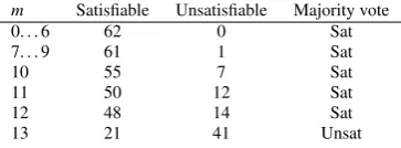
Table 3 Typical run for the Monty Hall example
m Satisfiable Unsatisfiable Majority vote
0. . . 6 62 0 Sat
7. . . 9 61 1 Sat
10 55 7 Sat
11 50 12 Sat
12 48 14 Sat
13 21 41 Unsat
the ratiomc(ϕacc)/mc(ϕterm), wheremc(·)denotes the model count of a formula, as in Section 2. Technically, we can use IA, the theory of integer arithmetic, with the domain
{1,2,3}for the free variablecand with the counting measure| · |:A7→ |A|, also following Section 2. So in our example,mc(ϕacc) =2 andmc(ϕterm) =3.
Computing the value of the program
We show how our method (see Subsection 3.2) estimatesmc(ϕacc). We make several copies of the variablec, denotedc1, . . . ,cq. The formula
ϕ(c) =ϕacc(c1)∧ϕacc(c2)∧. . .∧ϕacc(cq)
has 2qmodels, and we can estimatemc(ϕ
acc)by estimatingmc(ϕ)and taking theqth root of the estimate. Enlargingϕacc toϕ and then taking theqth root increases precision: for example, if the approximation procedure gives a result up to a factor of 2, theqth root of the estimate formc(ϕ)gives an approximation formc(ϕacc)up to a factor of 21/q.
Now observe that for a hash functionhwith values in{0,1}m, taken at random from an appropriate family, the expected model count of the formula
ϕ(c)∧(h(c) =0m) (2)
ismc(ϕ)·2−m. By a Chernoff bound argument, the model count is concentrated around the expectation. Our algorithm will, for increasing values ofm, sample random hash functions from an appropriate class, construct the formula (2), and give the formula to an SMT solver to check satisfiability. (Note that such formulas are purely existential—in variablescas well as inqcopies ofN.) With high probability, the firstm for which the sampled formula is unsatisfiable will give a good enough estimate ofmc(ϕ)and, by the reduction above, of
mc(ϕacc).
Let us give some concrete values to support the intuition. We encode the numberc∈ {1,2,3}in binary, asc≡c0c1. We makeq=12 copies, and this will ensure that we will obtain theexactvalue ofmc(ϕacc)by takingqth root ofmc(ϕ), whereϕis as above (for exact rather than approximate solution, a multiplicative gap of less than 3/2 suffices in our setting). In reality,mc(ϕacc) =2 and somc(ϕ) =212, but we only know a priori that
least 0.99 (see Appendix A for derivation of the constants 0.17 and 11.66). This gives us the interval[1.73,2.45]formc(ϕacc); sincemc(ϕacc)is integer, we conclude thatmc(ϕacc) =2 with probability at least 0.99.
As mentioned above, the same technique will deliver us mc(ϕterm) =3 and hence,
val(Switch) =2/3.
5 Value Estimation for Probabilistic Programs
In this section we show how our approach to #SMT applies to thevalue problemfor proba-bilistic programs.
What are probabilistic programs?
Probabilistic models such as Bayesian networks, Markov chains, probabilistic guarded-command languages, and Markov decision processes have a rich history and form the model-ing basis in many different domains (see, e.g., [22, 45, 16, 38]). More recently, there has been a move toward integrating probabilistic modeling with “usual” programming languages [25, 46]. Semantics and abstract interpretation for probabilistic programs with angelic and de-monic non-determinism has been studied before [39, 45, 47, 15], and we base our semantics on these works.
Probabilistic programming models extend “usual” nondeterministic programs with the ability to sample values from a distribution and condition the behavior of the programs based on observations [29]. Intuitively, probabilistic programs extend an imperative programming language like C with two constructs: a nondeterministic assignment to a variable from a range of values, and a probabilistic assignment that sets a variable to a random value sampled from a distribution. Designed as a modeling framework, probabilistic programs are typically treated as descriptions of probability distributions and not meant to be implemented and executed as usual programs.
Section summary
We consider a coreloop-freeimperative language extended withprobabilistic statements, similarly to [52], and withnondeterministic choice. Under each given assignment to the probabilistic variables, a program accepts (rejects) if there is an execution path that is com-patible with the observations and goes from the initial vertex to the accepting (resp., reject-ing) vertex of its control flow automaton. Consider all possible outcomes of the probabilistic assignments in a programP. Restrict attention to those that result inPreaching (nondeter-ministically) at least one of the accepting or rejecting vertices—such elementary outcomes form the setTerm(for “termination”); only these scenarios are compatible with the observa-tions. Similarly, some of these outcomes may result in the program reaching (again, nonde-terministically) the accepting vertex—they form the setAccept. Note that the setsTermand
Acceptare events in a probability space; defineval(P), thevalueofP, as the conditional probabilityPr[Accept|Term], which is equal to the ratio PrPr[Accept[Term]] asAccept⊆Term. We assume that programs are well-formed in thatPr[Term]is bounded away from 0.
Proposition 2 There exists a polynomial-time algorithm that, given a programPoverT, constructs logical formulasϕacc(R)andϕterm(R)overT such thatAccept=JϕaccKand
Term=JϕtermK, where each free variable r∈R is interpreted over its domain with measure
dist(r). Thus,val(P) =mc(ϕacc)/mc(ϕterm).
Proposition 2 reduces thevalue problem—i. e., the problem of computingval(P)—to model counting. This enables us to characterize the complexity of the value problem and solve this problem approximately using the hashing approach from Section 3. These results appear as Theorem 4 in Subsection 5.5 below.
In the remainder of this section we define the syntax (Subsection 5.1) and semantics (Subsection 5.2) of our programs and the value problem. By reducing this problem to #SMT (Subsection 5.5) we show an application of our approach to approximate model counting (an experimental evaluation is provided in Subsection 5.6). We also discuss modeling different kinds of nondeterminism: cooperative and adversarial (Subsection 5.3), and give an short overview of known probabilistic models subsumed by ours (Subsection 5.4).
5.1 Syntax
A program has a set of variablesX, partitioned into Boolean, integer, and real-valued ables. We assume expressions are type correct, i.e., there are no conversions between vari-ables of different types. Thebasic statementsof a program are:
– skip(do nothing),
– deterministic assignmentsx:=e,
– probabilistic assignmentsx∼Uniform(a,b), – assume statementsassume(ϕ),
whereeandϕcome from an (unspecified) language of expressions and predicates, respec-tively.
The (deterministic) assignment and assume statements have the usual meaning: the de-terministic assignmentx:=esets the value of the variablexto the value of the expression on the right-hand side, andassume(ϕ)continues execution only if the predicate is satisfied in the current state (i.e., it models observations used to condition a distribution). The prob-abilistic assignment operationx∼Uniform(a,b)samples the uniform distribution over the range[a,b]with constant parametersa,band assigns the resulting value to the variablex. For example, for a real variablex, the statementx∼Uniform(0,1)draws a value uniformly at random from the segment[0,1], and for an integer variabley, the statementy∼Uniform(0,1)
setsyto 0 or 1 with equal probability.
Thecontrol flowof a program is represented using directed acyclic graphs, called con-trol flow automata (CFA), whose nodes represent program locations and whose edges are labeled with program statements. LetS denote the set of basic statements; then acontrol flow automaton(CFA)P= (X,V,E,init,acc,rej)consists of a set of variablesX, a la-beled, directed, acyclic graph(V,E), withE⊆V×S×V, and three designated vertices
init,acc, andrejinVcalled theinitial,accepting, andrejectingvertices.
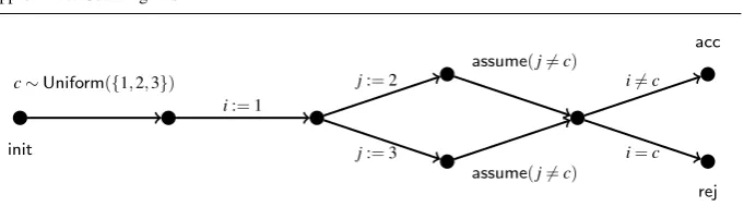
Figure 1 depicts the CFA for the probabilistic program shown in Procedure 3: “Switch” strategy in Monty Hall problem. Theacceptandrejectstatements from the procedure cor-respond to theaccandrejvertices of the CFA respectively.
We assumeinithas no incoming edges andaccandrejhave no outgoing edges. We write
init
acc
rej c∼Uniform({1,2,3})
i:=1
j:=2
j:=3
assume(j6=c)
assume(j6=c)
i6=c
i=c
Fig. 1 CFA for the probabilistic program given as Procedure 3: “Switch” strategy in Monty Hall problem.
that is, each variable is assigned at most once along any execution path. A program can be converted to SSA form using standard techniques [48, 31].
Since control flow automata are acyclic, our programs do not have looping constructs. Loops can be accommodated in two different ways: by assuming that the user provides loop invariants [35], or by assuming an outer (statistical) procedure that selects a finite set of executions that is sufficient for the analysis up to a given confidence level [52, 51]. In either case, the core analysis problem reduces to analyzing finite-path unwindings of programs with loops, which is exactly what our model captures.
Although our syntax only allows uniform distributions, we can model some other dis-tributions. For example, to simulate a Bernoulli random variablexthat takes value 0 with probabilitypand 1 with probability 1−p, we write the following code:
X∼Uniform(0,1);
if(X≤p){x:=0;}else{x:=1;}
We can similarly encode uniform distributions with non-constant boundaries as well as (ap-proximately encode) normal distributions (using repeated samples from uniform distribu-tions and the central limit theorem). To encode uniform distribudistribu-tions with non-constant boundaries, we useassumeconditioning: e.g., to simulate a random variablexthat has dis-tributionUniform(−y2,1+2y)wherey∈[0,10]is a previously assigned variable, we write the following code:
x∼Uniform(−100,21);
assume(−y∗y≤x≤1+2∗y);
The semantics of this conditioning is explained in the following subsection.
5.2 Semantics
The semantics of a probabilistic program is given as a superposition of nondeterministic programs, following [39, 15]. Intuitively, when a probabilistic program runs, an oracle makes all random choices faced by the program along its execution up front. With these choices, the program reduces to a usual nondeterministic program.
We first provide some intuition behind our semantics. Let us partition the variablesX of a program into random variablesR(those assigned in a probabilistic assignment) and nondeterministic variablesN=X\R(the rest). (The partition is possible because programs are in static single assignment form.) We consider two events. The (normal)termination
[image:22.595.78.419.74.169.2]inR, there is an assignment to the variables inN such that the program execution under this choice of values reachesaccorrej(resp. reachesacc). The termination is “normal” in that allassumes are satisfied. Our semantics computes the conditional probability, under all scenarios, of the acceptance event given that the termination event occurred.
We now formalize the semantics. Astateof a program is a pair(v,x)of a control node
v∈V and a type-preserving assignment of values to all program variables inX. LetΣ
denote the set of all states andΣ∗the set of finite sequences overΣ.
Let(Ω,F,Pr)be the probability space associated with probabilistic assignments in a program P; elements of Ωwill be called scenarios. The probabilistic semantics of P, denotedh[P]i, is a function fromΩto 2Σ
∗
, mapping each scenarioω∈Ωto a collection of
maximal executions of the nondeterministic program obtained by fixingω. It is defined with
the help of an extension ofh[·]ifrom programs to states, which, in turn, is defined inductively as follows:
– (acc,x)∈ h[acc]iωand(rej,x)∈ h[rej]iωfor allx;
– (v,x)(v0,x)σ∈ h[v]iωifv−−→skip v0and(v0,x)σ∈ h[v0]iω;
– (v,x)(v0,x0)σ ∈ h[v]iω ifv−−→x:=e v0,x0=x[x:=eval(e)(x,ω)], and(v0,x)σ∈ h[v0]iω; similarly, ifv−−−−−−−−−→x∼Uniform(a,b) v0, we havex0=x[x:=c]wherecis the value chosen forx
in the scenarioω;
– (v,x)(v0,x)σ∈ h[v]iωifv
assume(ϕ)
−−−−−−→v0,eval(ϕ)(x,ω) =true, and(v0,x)σ∈ h[v0]iω.
Finally, defineh[P]iω=h[init]iω. Hereeval(e)(x,ω)(resp.eval(ϕ)(x,ω)) denotes the value of the expressione(resp. predicateϕ) taken in the scenarioωunder the current assignment xof values to program variables, andx[x:=c]is the assignment that maps variablexto the valuecand agrees withxon all other variables.
LetΦ⊆Σ∗be a set of paths of a programP. The probability that the run ofPhas a
propertyΦis defined as
Pr[run ofPsatisfiesΦ] = Z
Ω
1
h[P]i ∩Φ6=/0dPr(ω)
where1
h[P]i ∩Φ6=/0denotes the indicator event that at least one execution path from
h[P]ibelongs toΦ. Specifically, letΦacc⊆Σ∗be the set of all sequences that end in a state
(acc,x)for somex, andΦterm⊆Σ∗be the set of all sequences that end in either(acc,x)or
(rej,x). We define theterminationandacceptanceevents as
Term= [run ofPsatisfiesΦterm],
Accept= [run ofPsatisfiesΦacc].
Thevalueval(P)of a programP is defined as the conditional probabilityPr[Accept|
Term], which is equal to the ratioPrPr[Accept[Term]] asAccept⊆Term. Thus, the value of a program is the conditional probability
Prω[∃z.P(ω,z)reachesacc| ∃z.P(ω,z)reachesaccorrej].
For simplicity of exposition, we restrict attention to well-formed programs, for whichPr[Term]
is bounded away from 0. Thevalue problemtakes as input a program P and computes
val(P).
5.3 Cooperative vs. adversarial nondeterminism
Our semantics corresponds to acooperativeunderstanding of nondeterminism, in the fol-lowing sense. For each individual scenarioω, the seth[P]iωcan have one of the following four forms:
1) there are no paths toaccnorrej(for any assignmentzfor the nondeterministic variables inN),
2) there is a path torej, but no paths toacc, 3) there is a path toacc, but no paths torej,
4) there are paths to bothaccandrej(under different assignmentsz,z0for the nondeter-ministic variables).
The conditional probability measure
Prω[· |Term] =Prω[· | ∃z.P(z,ω)reachesaccorrej]
restricts the attention toω of the forms 2, 3, 4. Now our definition ofAcceptsays that all
ωof the form 4 are counted towards acceptance. The value of the program is accordingly
defined as the (conditional) probability of options 3, 4.
In the Monty Hall problem in Section 4, this semantics worked as intended only be-cause there are no scenariosωof the form 4. However, a cooperative interpretation may not always be desirable. Imagine, for instance, that in a game, for some fixed strategy of the player all scenariosωhave the form 4, which means that the outcome of the game depends
on the host’s choice. Our semantics evaluates the strategy as perfect, with the value 1, al-though using the strategy may even lead tolosingwith probability 1 once nondeterminism is interpreted adversarially.
We can distinguish between semantics with cooperative and adversarial (also known as angelic and demonic) nondeterminism by defining theupperandlowervalues of a program by
val(P) =Prω[∃z.P(z,ω)reachesacc|Term] and
val(P) =Prω[@z.P(z,ω)reachesrej|Term].
The upper valueval(P)coincides withval(P)as defined in Subsection 5.2, and the lower valueval(P)indeed corresponds to the adversarial interpretation of nondeterministic choice: only scenarios of the form 3 are counted towards acceptance, and scenarios of the form 2 and, most importantly, 4 towards rejection. Obviously,val(P)≤val(P), with equality if and only if the set of scenarios of the form 4 has (conditional) measure zero, as in Section 4. Observe now that the problem of computingval(P)reduces to the problem of comput-ingval(P): the reason for that is the equality
val(P) =1−val(P∗),
where for a programP= (X,V,E,init,acc,rej)we define the correspondingdualprogram P∗= (X,V,E,init,rej,acc). The details are easily checked.