warwick.ac.uk/lib-publications
Original citation:
Goddard, C. R., Pascoe, D. J. (David J.), Anfinogentov, Sergey and Nakariakov, V. M. (Valery
M.). (2017) A statistical study of the inferred transverse density profile of coronal loop
threads observed with SDO/AIA. Astronomy & Astrophysics
Permanent WRAP URL:
http://wrap.warwick.ac.uk/88923
Copyright and reuse:
The Warwick Research Archive Portal (WRAP) makes this work by researchers of the
University of Warwick available open access under the following conditions. Copyright ©
and all moral rights to the version of the paper presented here belong to the individual
author(s) and/or other copyright owners. To the extent reasonable and practicable the
material made available in WRAP has been checked for eligibility before being made
available.
Copies of full items can be used for personal research or study, educational, or not-for-profit
purposes without prior permission or charge. Provided that the authors, title and full
bibliographic details are credited, a hyperlink and/or URL is given for the original metadata
page and the content is not changed in any way.
Publisher’s statement:
“Reproduced with permission from Astronomy & Astrophysics, © ESO 2017”.
A note on versions:
The version presented here may differ from the published version or, version of record, if
you wish to cite this item you are advised to consult the publisher’s version. Please see the
‘permanent WRAP URL’ above for details on accessing the published version and note that
access may require a subscription.
June 5, 2017
A statistical study of the inferred transverse density profile of
coronal loop threads observed with SDO/AIA
C. R. Goddard
1, D. J. Pascoe
1, S. Anfinogentov
1, and V. M. Nakariakov
1,21 Centre for Fusion, Space and Astrophysics, Department of Physics, University of Warwick, CV4 7AL, UK, e-mail: [email protected]
2 School of Space Research, Kyung Hee University, 446-701 Yongin, Gyeonggi, Korea
Received ???? 2017/Accepted ???? 2017
ABSTRACT
Aims.We carry out a statistical study of the inferred coronal loop cross-sectional density profiles using extreme ultraviolet (EUV) imaging data from the Atmospheric Imaging Assembly (AIA) on board the Solar Dynamics Observatory (SDO).
Methods.We analysed 233 coronal loops observed during 2015/2016. We consider three models for the density profile; the step function (modelS), the linear transition region profile (modelL), and a Gaussian profile (modelG). Bayesian inference is used to compare the three corresponding forward modelled intensity profiles for each loop. These are constructed by integrating the square of the density from a cylindrical loop cross section along the line of sight, assuming an isothermal cross section, and applying the instrumental point spread function.
Results.Calculating the Bayes factors for comparisons between the models, it was found that in 47 % of cases there is very strong evidence for modelLover modelSand in 45 % of cases very strong evidence for modelGoverS. Using multiple permutations of the Bayes factor the favoured density profile for each loop was determined for multiple evidence thresholds. There were a similar number of cases where modelLorGare favoured, showing evidence for inhomogeneous layers and constantly varying density cross sections, subject to our assumptions and simplifications.
Conclusions.For sufficiently well resolved loop threads with no visible substructure it has been shown that using Bayesian inference and the observed intensity profile we can distinguish between the proposed density profiles at a given AIA wavelength and spatial resolution. We have found very strong evidence for inhomogeneous layers, with model Lbeing the most general, and a tendency towards thicker or even continuous layers.
Key words.Sun: corona - Sun: oscillations - methods: observational
1. Introduction
The solar corona is highly structured, due to a combination of the low-βplasma parameter and the magnetic field that pene-trates it from the lower atmosphere. The hot coronal plasma ap-pears to fill in the magnetic flux tubes in certain locations, nor-mally within active regions, forming the curved coronal loops and threads observed by extreme ultraviolet (EUV) imagers. The precise nature of coronal loop formation, and their transverse and longitudinal structure is still debated. The transverse den-sity structure of coronal loops is currently of high importance, as outlined below, and is the focus of this study.
There have been multiple studies of the transverse structure of coronal loops with each generation of EUV imagers (e.g. Bray & Loughhead 1985; Aschwanden & Nightingale 2005; Aschwanden & Boerner 2011; Peter et al. 2013). The major-ity of such studies note that the transverse intensmajor-ity profile of the loops resembles a Gaussian peak, which is used to estimate the loop position, width and intensity contrast. To infer the den-sity structure from these intenden-sity profiles the relationship be-tween the density profile of a coronal loop and its appearance in EUV images needs to be understood. The emission in a par-ticular spectral range in the EUV band depends on the plasma density and temperature. Additionally, coronal plasma is opti-cally thin and so multiple structures along the observational line of sight (LOS) will be superimposed in the observations. Finally,
the characteristics of the instrument should also be taken into ac-count.
Coronal loops are generally considered to consist of a core of uniform density with an inhomogeneous layer surrounding it. Using data from the Transition Region And Coronal Explorer (TRACE;Handy et al. 1999),Aschwanden et al.(2003) mea-sured the thickness of the non-uniform layer for multiple loops based on a density profile with a sinusoidal transition layer and a uniform core. When the effects of the relationship between the intensity and density, LOS integration and the instrumen-tal point spread function (PSF) were included this density pro-file was capable of reproducing the observed intensity propro-file. Aschwanden et al.(2007) performed a large scale study of the transverse structure of loops, using intensity profiles based on step function and constantly varying density profiles.
Analysed loops have been found to range from near isother-mal to highly multi-therisother-mal. Aschwanden & Boerner (2011) performed a systematic study of the cross-sectional tempera-ture structempera-ture of coronal loops using the Atmospheric Imaging Assembly (AIA) on the Solar Dynamics Observatory (SDO; Lemen et al. 2012), finding evidence for near isothermal loop cross-sections. High-resolution Coronal Imager (Hi-C) data was used to measure the Gaussian widths of multiple loops, finding a distribution that peaked at 270 km, the temperature distributions were also found to be narrow (Brooks et al. 2013). Further ex-amples for narrow temperature ranges in coronal loops include (e.g.Warren et al. 2008). However, there are examples of
Goddard et al.: Coronal loop density profiles - a statistical study
thermal loops (Schmelz et al. 2010;Nistic`o et al. 2014a,2017) and active, or flaring, loops should also be multi-thermal.
The unresolved sub-structure of coronal loops is also de-bated, i.e.loops (or threads) which appear monolithic may be comprised of multiple smaller threads with a certain filling fac-tor. Despite numerous studies using multiple instruments no clear consensus has been reached (e.g.Reale et al. 2011;Brooks et al. 2012;Peter et al. 2013;Brooks et al. 2016;Krishna Prasad et al. 2017). However, it appears the lower limit of thread widths is close to being resolved, with a lower limit of 100 km predicted (Aschwanden & Peter 2017).
The transverse structure of coronal loops can be determined from, and is integral to, the study of the oscillations they ex-hibit. Kink, or transverse, oscillations of coronal loops are one of the most intensively studied examples of magnetohydrody-namic (MHD) waves in the Solar system. These waves have been clearly observed by EUV imagers such as AIA. The initial detec-tions (Aschwanden et al. 1999;Nakariakov et al. 1999) showed rapid damping, and this is now attributed to resonant absorption (e.g.Ruderman & Roberts 2002;Goossens et al. 2002). This the-ory is dependant on the existence of a non-uniform layer, where there is a transition between the density inside and outside the loop. The gradient of the Alfv´en speed, and therefore the trans-verse density profile, then determines the spatial and temporal scales over which the waves are dissipated and the energy is deposited (e.g Heyvaerts & Priest 1983; Cally 1991; Soler & Terradas 2015). The phase mixing length scale defined byMann et al.(1995) was reproduced by numerical simulations of propa-gating kink waves (Pascoe et al. 2010), while the corresponding Alfv´en wave lifetime has been seismologically calculated using standing kink waves (Pascoe et al. 2016a).
Large scale statistical studies of kink oscillations (Zimovets & Nakariakov 2015; Goddard et al. 2016) have recently been performed. This work lead to the confirmation of the presence of non-exponential damping envelopes of some of the oscilla-tions studied (Pascoe et al. 2016b). This can be attributed to the damping profile proposed in Pascoe et al.(2012,2013), which has subsequently been used to perform seismology, including the use of Bayseian model comparison (Pascoe et al. 2016a,2017a). InPascoe et al.(2017b) the result of this seismology was com-pared to density profiles estimated from the EUV intensity for one coronal loop. Arregui et al.(2015) considered the depen-dence of seismological information on the inhomogeneous layer density profile, without the use of the non-exponential section of the damping envelope, meaning inversion curves were obtained and compared for the different density profiles.
The transverse density structure can also play an important role in understanding and detecting nonlinear effects.Terradas et al.(2008) performed a nonlinear numerical study of kink os-cillations, finding that shear instabilities develop and deform the boundary of the loop. They related their results to the devel-opment of the Kelvin-Helmholtz instability (KHI) for torsional Alfv´en waves, which was first described byBrowning & Priest (1984). Further numerical studies of the KHI instability for os-cillating structures in the corona include; flux tubes (Soler et al. 2010), transverse prominence oscillations (Antolin et al. 2015) and coronal loops (Antolin et al. 2016). In all of these exam-ples the transverse structure is perturbed, which is of theoretical and observational significance. Recently, a study of kink oscil-lations of coronal loops showed a negative correlation between the quality factor of the oscillations and the amplitude, suggest-ing the presence of nonlinear effects at moderate to large am-plitudes, causing real or apparent additional damping (Goddard & Nakariakov 2016). A similar dependence was found in a
nu-merical study byMagyar & Van Doorsselaere(2016a), in which non-linear mechanisms such as KHI were found to modify the damping of the kink mode significantly at large amplitudes.
The specific shape of the transverse non-uniformity is also responsible for the geometrical dispersion of the fast magnetoa-coustic waves guided by the loop, which determines the spe-cific shape of the quasi-periodic rapidly propagating wave trains (Nakariakov et al. 2004; M´esz´arosov´a et al. 2014; Yu et al. 2016). These wave trains have recently been detected in the corona with the EUV imagers (e.g.Liu et al. 2011;Nistic`o et al. 2014b), and the full realisation of their seismological potential requires the knowledge of the transverse profile of the waveg-uiding plasma nonuniformity.
In understanding the mechanisms and effects discussed above, as well as the seismology which is based on them, it is im-portant to understand the transverse and longitudinal loop struc-ture, combining knowledge of the formation and structure of coronal loops and the oscillations they exhibit. In this paper we consider a sufficiently simplified forward modelling procedure which allows us to test which transverse density profile has the most evidence for individual loops based on their observed in-tensity profile using Bayesian inference. In addition, the structur-ing parameters with the greatest evidence are obtained for each density model. Our model comparison approach, described in Section 3, is the same as that described inPascoe et al.(2017a). The paper is organised as follows; in Section 2 the observa-tions and data are described, in Section 3 the forward modelling and model comparison methods are outlined, in Section 4 the re-sults are presented, and the discussion and conclusions are given in Sections 5 and 6.
2. Observations
For this study we are neglecting any time dependent evolution of the loops. For this reason we use single AIA images at 171, 193 and 211 Å. One set of images was downloaded for each week be-tween January 2015 and September 2016. Each image was plot-ted, and loops or threads which appeared monolithic and had a well contrasted segment were identified. This may be an individ-ual thread (or strand), which is part of a larger loop bundle, as long as the width of the thread is sufficient for us to resolved the cross sectional structure. Two points were selected either side of the loop at a position which minimised background contamina-tion from other structures and maximised the intensity contrast. The intensity was extracted along a line connecting these two points, and was averaged over a width of 5 pixels. The uncer-tainty and noise on these intensity profiles are considered to be unknown and were inferred during the analysis we describe be-low. This process resulted in 233 loops for further analysis.
We acknowledge that our sample of loops is not unbiased as loops or threads with a sufficient width to be well resolved and which had no visible sub-structure were selected. Higher, or longer, coronal loops are under sampled, due to the increased noise and reduced intensity contrast making them unsuitable for our analysis.
It was found that the correlation between the loops inten-sity profile at 171 Å and the other two wavelengths was low in general, implying that the structures studied are not generally multi-thermal over the temperatures sampled by the chosen AIA passbands (which does not exclude them being multi-thermal within a narrower temperature range, or threads with different peak temperatures that are not co-spatial). In general, it did not appear that the intensity profiles at 193 and 211 corresponded to
the hotter outer layer counterpart of a cooler core seen in 171, which is often assumed to be the case in forward modelling (e.g. Magyar & Van Doorsselaere 2016b;Antolin et al. 2016). For this reason we do not extend our analysis to the other wavelengths, and this should be the subject of further study.
3. Method
3.1. Constructed intensity profiles
In this study we consider three models for the cross-sectional density profile of the coronal loops; the step function profile, the transition layer profile, and the Gaussian profile as described and motivated inPascoe et al.(2017b). The generalised Epstein profile is not used as the two limits of this profile are well rep-resented by the transition layer profile and the Gaussian profiles. InPascoe et al. (2017b) it was found that the advantage of the Epstein profile, over the layer profile, as reflected in the Bayes factor, was negligible.
The step function profile (modelS) is described by an in-ternal densityρ0, the external densityρe, and a minor radiusR. In this case the transverse density profileρprqfor a loop with a cylindrically symmetric cross-section and radial coordinateris given by
ρprq “
"
A, |r| ďRS
0, |r| ąRS , (1)
whereA“ρ0´ρeis the loop density enhancement.
We also consider a Gaussian density profile (modelG) given by
ρprq “Aexp
˜
´ r
2
2R2G
¸
. (2)
The linear transition layer profile (modelL) is given by
ρprq “
$ ’ &
’ %
A, |r| ďr1
A
´
1´ r´r1
r2´r1
¯
, r1ă |r| ďr2 0, |r| ąr2
(3)
wherer1 “RLp1´{2q,r2“RLp1`{2q, and“l{Ris the transition layer widthlnormalised toRand defined to be in the rangeP r0,2s. Examples of the three model density profiles are given in the right hand panels of Fig.1for three of the analysed loops.
The use of the isothermal approximation allows the intensity profile to be calculated as the square of the density integrated along the LOS. We calculate the loop intensity profile numeri-cally by constructing a 2D density profile for the radial profiles
given in Eqs. (1) – (2) withr“
b
px´x0q2` py´y0q2,where
xis the coordinate transverse to the loop, with the loop centre at x0, andyis the coordinate along the LOS.
In addition to the contribution from the loop given by Eqs. (1)–(2), the density profile also includes a background com-ponent which is described by a second order polynomial. This is included to model the emission from the background plasma and other structures along the LOS. The instrumental PSF is then applied using a Gaussian kernel withσ “1.019 pixels, corre-sponding to the 171Å SDO/AIA channel (Grigis et al. 2013). The 2D density profile is constructed with 10 times the resolu-tion of the observed intensity profile. The model intensity pro-files (L,GandS) are then interpolated onto the observational co-ordinates and compared with the observed intensity profile using the method outlined below.
3.2. Bayesian inference
We follow the model comparison procedure based on Bayesian inference and Markov chain Monte Carlo (MCMC) sampling de-scribed in Pascoe et al. (2017a) and applied to a coronal loop intensity profile inPascoe et al.(2017b).
For this procedure priors need to be selected for each of the parameters. An initial least squares fit is performed on the inten-sity profiles using the forward modelled inteninten-sity profile from density profileL. This allows guess parameters to be obtained, allowing suitable limits on the priors to be obtained for the x position, radius and intensity contrast of the loop and the back-ground polynomial. For the layer profile we prescribe 0ďď2 according to the definition of our density profile. The prior prob-ability distributions of all the above parameters are taken to be constant within the prescribed bounds.
Any two modelsMiandMjmay be quantitatively compared using the Bayes factor, defined as
Bi j“
PpD|Miq
PpD|Mjq
, (4)
where the evidences, PpD|Mq are calculated as described in Pascoe et al.(2017a). To define evidence thresholds the natural logarithm of this factor, i.e.
Ki j“2 lnBi j, (5)
is considered, where values ofKi jgreater than 2, 6 and 10 cor-respond to “positive”, “strong”, and “very strong” evidence for modelMiover modelMj, respectively. Negative values indicate evidence for modelMjsubject to the same thresholds. We con-sider all permutations of the Bayes factor for ModelsS,Land G.
For the purpose of prescribing which model is favoured for each intensity profile, and to what degree, we define the proba-bility of a given model using normalisation of the evidence val-ues as
Pi“
Ei
ES`EL`EG
, (6)
where Pi andEi are the probability and evidence for a given model andES,EL, andEGare the evidence values for models S, L and G as described above.
To plot intensity profiles for the models, and plot the dis-tributions of the parameters of interest, we obtain estimates and uncertainties for the model values by taking the median and 95th percentile of the probability distributions for a given parameter.
4. Results
4.1. Model Comparisons
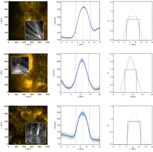
We analysed 233 coronal loops using the method described in Sect. 2, and obtained Bayes factors, Ki j, and the probability of each model, Pi, for each loop. Three examples are shown in Fig. 1. The top row shows a loop for which model L was favoured. The corresponding Bayes factors and model probabil-ities areKLS=32.3,KLG=26.6,KGS=5.7 andPL=1.00,PG=0.00,
Goddard et al.: Coronal loop density profiles - a statistical study
Fig. 1.Examples of loops for which modelsL(top),G(middle), andS (bottom) were found to best describe the data.LeftSDO/AIA
171 Å image of an analysed loop. The blue lines indicates the location of the slits used to generate the transverse intensity profiles. The white box and inset show a magnified region around the loop. Middle 171 Å EUV intensity profile (symbols) across the selected loop. ModelL (blue line) is plotted, with the model values being the median values from the corresponding probability distributions. The shaded areas represent the 99% confidence region for the intensity predicted by the model, with (red) and without (blue) modelled noise.The vertical dotted and dashed lines denote x0andx0˘R, respectively.RightThe returned density profiles for modelsS (solid),L(dashed) andG(dotted).
blue respectively). On the right the returned density profiles for modelsS (solid),L(dashed) andG(dotted) are plotted.
The middle row shows a loop for which model G was favoured. The corresponding Bayes factors and model prob-abilities are KLS=46.5, KLG=-13.5, KGS=60.0 and PL=0.01,
PG=0.99, PS=0.00. The bottom row shows a loop for which model S was favoured. The corresponding Bayes factors and
model probabilities are KLS=-2.29, KLG=16.5, KGS=-18.4 and
PL=0.24, PG=0.00, PS=0.76. We note that this loop has the smallest radius, and therefore the lowest spatial information.
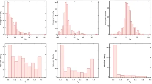
In Fig.2histograms of the Bayes factorsKLS,KGS andKLG are plotted. The values of KLS are seen to be largely positive, indicating that ModelLis almost always a better model for the density profile of the coronal loops analysed than ModelS, given
Fig. 2.Top rowHistograms of the Bayes factor (Ki j) comparisons of ModelsL,GandS.Bottom rowHistograms of the model probabilities (Pi) calculated from the evidence values for each model.
Table 1.Percentages of cornal loop intensity profiles falling into
three evidence thresholds for each permutation of the Bayes fac-tor for modelsL,GandS.
Ki j>2 Ki j>6 Ki j>10
KLS 75 % 58 % 47 %
KS L 4 % 0 % 0 %
KGS 65 % 53 % 45 %
KS G 25 % 25 % 12 %
KLG 42 % 24 % 15 %
KGL 32 % 12 % 5 %
our assumptions. The values ofKGS are more evenly distributed about zero, indicating that the use of ModelGover ModelS is not always justified, however there is strong evidence for it in many cases. Finally, the values ofKLGare also distributed about zero, with a slight bias to positive values, indicating many loops show strong evidence for either of the profiles over the other.
These results are better quantified by considering the ev-idence thresholds stated in Sect. 2. These are summarised in Table1forKLS,KLG andKGS. Each permutation of the Bayes factor is included, with the main result being that in 47 % of cases there is very strong evidence for model L over modelS and in 45 % of cases very strong evidence for modelGoverS.
These thresholds can be used to determine which of the three models is favoured for each loop, and how strongly. In Table2
[image:6.595.375.499.474.548.2]percentages of loops falling into each evidence threshold for each model are listed. For a loop to be counted for a given model i, and threshold its Bayes factor for the comparison to the other two models, Bi j andBik must be greater than the threshold. In this case there is a competition between models, so only 5 %
Table 2.Rows 1-4Percentages of coronal loop intensity profiles
falling into three evidence thresholds for each density model. For a loop to be counted for a given model and threshold it’s Bayes factor from comparison to both other models,Ki jandKik, must be greater than that threshold.Row 5Summed probability values (Pi) for each density model, showing how the evidence is distributed between the three models for our 233 analysed loops.
L G S
>0 44 % 43 % 13 % >2 25 % 32 % 4 % >6 8 % 12 % 0 % >10 5 % 5 % 0 % ř
Pi 101.5 99.4 32.1
of loops have very strong evidence for modelLorGover both other respective models.
The probabilities calculated for each model for each loop, Pi, can be summed to show how the evidence is distributed be-tween the three models. These values are 101.5, 99.4 and 32.1 for modelL,GandS respectively, given in Table2. This again shows the similarly strong evidence for modelsLandG.
The bottom row of Fig.2shows histograms ofPL,PGand
Goddard et al.: Coronal loop density profiles - a statistical study
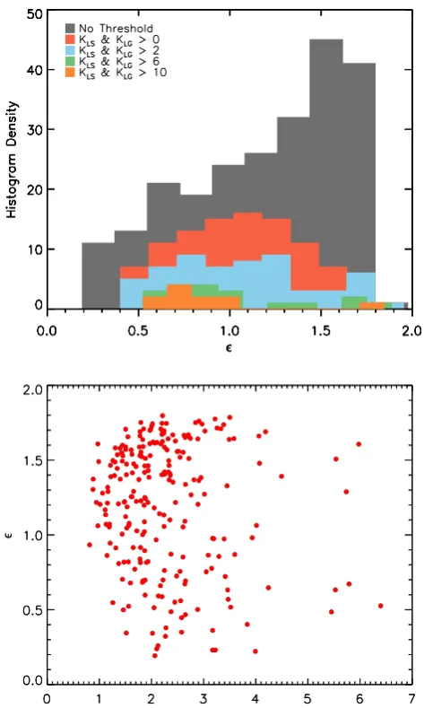
Fig. 3. UpperHistograms of the normalised layer widthfor the
combined thresholds ofKLSandKLGgiven in Tab.1.LowerThe normalised layer width,, plotted against the loop minor radius for modelL,RL.
4.2. Parameter dependencies
The upper panel of Fig.3shows histograms offor modelLfor the different thresholds ofKLS andKLGgiven in Table2(red to orange), and with no threshold (grey). These values correspond to the median values from the probability distributions of the parameter. It can be clearly seen that adding the threshold re-moves the cases where modelGwas favoured (corresponding to a higherfor modelL), shifting the distribution to lower values. The cases where modelS was favoured are also removed for the higher thresholds, removing the lower values of. In the lower panel of Fig.3is plotted against the radius for the layer model, RL, and shows no correlation. The values ofRLalso corresponds to the median values of the probability distribution.
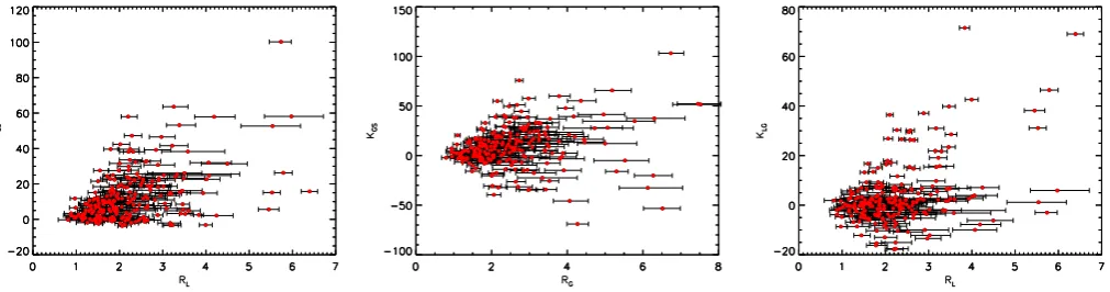
The left hand panel of Fig.4 shows the distribution of the radii for modelS,RS. This shows that the sampled loops have radii peaking at 2 Mm with a number of cases with higher radii. The middle panel plotsRLagainstRS, where the blue line corre-sponds toRL=RS and the right panel plotsRGagainstRS, where the blue line corresponds toRG=RS. This shows that despite the
evidence values for the different models varying the radii for the different models remain within error. It can be seen that model Gslightly overestimates the radius compared toS andL.
In Fig.5 KLS,KGS andKLG are plotted againstRL,RGand
RL respectively, showing that the spread of Bayes factors in-crease with loop radius due to the inin-creased spatial information. It can also be noted thatKLS is largely positive, whereasKGS is more evenly split between positive and negative values, but with higher values of both.KLGis also more evenly split between pos-itive and negative values, but with the highest evidence values for modelL(positiveKLG).
5. Discussion
Our results show that in the majority of cases there is evidence for a density profile with an inhomogeneous layer, and in the majority of loops selected there is enough spatial information to constrain the size of the inhomogeneous layer, or note a con-tinually varying profile being preferred. The existence of this inhomogeneous layer between the high density core and lower density background is a necessary and sufficient condition for resonant absorption to occur. It is therefore crucial to the inter-pretation of transverse loop oscillations in terms of kink oscil-lations damped by the coupling to Alfv´en waves inside the in-homogeneous layer, and hence the validity of any seismological calculations based on this interpretation.
The three cases in Fig.1highlight how the different density profiles considered behave for different loops. For the case where model L is favoured modelS sets the radius to occur halfway through the inhomogeneous layer and has a correspondingly re-duced density contrast. ModelGtends to overestimate the width and height of the density profile to match the gradient in the layer of model L. For the case where modelG is favoured modelL reproduces the profile well by minimising the size of the homo-geneous core. For the case where modelS was favoured model Lmatches the profile by minimising the size of the inhomoge-neous layer. ModelLtends to modelS in the limit Ñ0, and so for these cases the additional parameter, i.e., is redundant and so model S is naturally preferred in terms of the Bayesian evidence.
From our results we can see that despite model G being favoured strongly in some cases model L is the most general as it can reproduce both modelS andGsatisfactorily, while pro-viding additional information where there is evidence for an in-homogeneous layer and in-homogeneous core. This is encourag-ing for seismology beencourag-ing performed with modelL(Pascoe et al. 2016a), which is the only density profile for which the full ana-lytical solutions are known (Hood et al. 2013) for damping via resonant absorption. However, the many cases in which there is evidence for very large transition layers (or Gaussian density profiles), the thin boundary approximation used would no longer hold. For finite inhomogeneous layers, the damping rate (for the exponential damping regime) is modified by up to 25 % in com-parison with the thin boundary approximation (Van Doorsselaere et al. 2004). This may also have implications for the damping and dissipation of the Alfv´en waves generated via the resonant absorption of kink fast magnetoacoustic waves. The transverse Alfv´en speed profile asociated with the density profile may vary both the energy dissipation rate and it’s spatial distribution.
The tables and histograms of the Bayes factorsKi jand prob-abilities Pishow that there are a similar number of cases were ModelLorGare favoured over the other two, with many extend-ing into the “ very strong ” evidence threshold. From the bottom
Fig. 4.Comparison of the loop minor radius determined by our three models.LeftDistribution of the median radii from modelS, RS.MiddleThe loop radii from modelL,RL, plotted againstRS.RightThe loop radii from modelG,RG, plotted againstRS. The blue lines correspond toRL=RS andRG=RS respectively. The error bars correspond to the 95th percentile.
Fig. 5. LeftBayes factorKLS plotted against loop radiusRL.MiddleBayes factorKGS plotted against loop radiusRG.RightBayes
factorKLGplotted against loop radiusRL.
panel of Fig. 2, it can be seen thatPLis evenly distributed com-pared to PG, which is more confined to low and high values, reflecting the higher generality of modelLas discussed above.
From the histogram of the distribution without a thresh-old (grey) shows that the loops analysed generally have large or continuous inhomogeneous layers (were modelGwas favoured), in contrast to the typically small boundary layers considered in numerical modelling. For the first two thresholds the distribu-tion then centres aroundl“R. InMagyar & Van Doorsselaere (2016a) it was shown that for thick boundary layers ( >0.5) there is little or no effect on the exponential damping time at higher amplitudes. However for smaller layers ( <0.5) the am-plitude can have a strong effect on the observed damping time. Our results indicate that loops have inhomogeneous layers which fall on both sides of this threshold, however thicker layers appear to be far more common.
It should be noted that the cases where model S were favoured often corresponded to thinner loops or threads with lower minor radii. This reduction in the spatial information may cause modelS to be favoured irrespective of the actual density profile. In some cases the background intensity was not fit well by the second order polynomial, however this is the same for each profile and is reflected in the 99% confidence levels shown in the middle panels of Fig.1. It was found that using higher or-der polynomials for the background trend could lead to different models fitting different portions of the intensity profile, invali-dating their comparison.
Our use of the isothermal approximation means that any tem-perature variation across the loop that is sufficient to vary the
re-sponse function of the AIA channel analysed will be interpreted as a density variation. This may have contributed to the preva-lence of thick or continuous inhomogeneous layers obtained. However, considering the low correlation between the profiles seen in 171 Å and the hotter channels, the structures analysed at 171 Å may have a sufficiently narrow temperature distribution, with separate loops or threads existing in the hotter channels at similar, but not co-spatial, locations.
[image:8.595.53.559.253.386.2]Goddard et al.: Coronal loop density profiles - a statistical study
6. Conclusions
In summary, we have analysed the intensity cross-section of coronal loops (and/or threads) observed at 171 Å by SDO/AIA. In this channel typical non-flaring coronal loops are seen with the highest clarity and contrast. Assuming an isothermal and cylindrical cross-section we have inferred the transverse density structure of the coronal loop plasma which lies within the tem-perature range corresponding to 171 Å SDO/AIA channel.
Accounting for the instrumental PSF and integration along the LOS, very strong evidence was found for the existence of an inhomogeneous layer where the density varies smoothly be-tween the rarified background plasma and the dense centre of the loop. In many cases, the width of this layer was high enough to conclude that the loop does not have a core at all, and has a continuously varying density which may be better modelled by a Gaussian profile. This may have implications for the thin boundary approximation often used in the analytical description of oscillating loops. ModelLis found to be the most general as it can represent loops with no boundary layer as well as loops with a continuously varying density profile.
We acknowledge that several assumptions have been made to obtain these results. The study of multiple wavelengths, and the inclusion of the instrumental response function and a non-isothermal model for the loop cross-section require further work. The potential presence of unresolved sub-structure, and how this would manifest itself in our observations should also be consid-ered further. We have also assumed the loop is static during the exposure time of the instrument. If they oscillate with a period shorter than the exposure time, or move during the exposure, we would observe some apparent diffusion of its boundary.
From our analysis it is clear that using a linear boundary layer density profile, forward modelled to the resulting intensity profile, produces more information than the Gaussian intensity profiles typically used to fit and track coronal loops. Even with simple least squares fitting, when the spatial resolution is suf-ficient, this profile would provide information about the size of the inhomogeneous layer compared to the minor radius, and de-couples the measured minor radius from the intensity contrast.
Acknowledgements. The work was supported by the European Research Council under the SeismoSun Research Project No. 321141 (CRG, DJP, SA, VMN). We thank G. Nistic`o for useful discussions which helped seed the initial idea. The data is used courtesy of the SDO/AIA team.
References
Anfinogentov, S. A., Nakariakov, V. M., & Nistic`o, G. 2015, A&A, 583, A136 Antolin, P., De Moortel, I., Van Doorsselaere, T., & Yokoyama, T. 2016, ApJ,
830, L22
Antolin, P., Okamoto, T. J., De Pontieu, B., et al. 2015, ApJ, 809, 72 Arregui, I., Soler, R., & Asensio Ramos, A. 2015, ApJ, 811, 104 Aschwanden, M. J. & Boerner, P. 2011, ApJ, 732, 81
Aschwanden, M. J., Fletcher, L., Schrijver, C. J., & Alexander, D. 1999, ApJ, 520, 880
Aschwanden, M. J. & Nightingale, R. W. 2005, ApJ, 633, 499
Aschwanden, M. J., Nightingale, R. W., Andries, J., Goossens, M., & Van Doorsselaere, T. 2003, ApJ, 598, 1375
Aschwanden, M. J., Nightingale, R. W., & Boerner, P. 2007, ApJ, 656, 577 Aschwanden, M. J. & Peter, H. 2017, ArXiv e-prints [[arXiv]1701.01177] Bray, R. J. & Loughhead, R. E. 1985, A&A, 142, 199
Brooks, D. H., Reep, J. W., & Warren, H. P. 2016, ApJ, 826, L18 Brooks, D. H., Warren, H. P., & Ugarte-Urra, I. 2012, ApJ, 755, L33
Brooks, D. H., Warren, H. P., Ugarte-Urra, I., & Winebarger, A. R. 2013, ApJ, 772, L19
Browning, P. K. & Priest, E. R. 1984, A&A, 131, 283 Cally, P. S. 1991, Journal of Plasma Physics, 45, 453 Goddard, C. R. & Nakariakov, V. M. 2016, A&A, 590, L5
Goddard, C. R., Nistic`o, G., Nakariakov, V. M., & Zimovets, I. V. 2016, A&A, 585, A137
Goossens, M., Andries, J., & Aschwanden, M. J. 2002, A&A, 394, L39 Grigis, P., Yingna, S., & Weber, M. 2013, Tech. Rep., AIA team
Handy, B. N., Acton, L. W., Kankelborg, C. C., et al. 1999, Sol. Phys., 187, 229 Heyvaerts, J. & Priest, E. R. 1983, A&A, 117, 220
Hood, A. W., Ruderman, M., Pascoe, D. J., et al. 2013, A&A, 551, A39 Krishna Prasad, S., Jess, D. B., Klimchuk, J. A., & Banerjee, D. 2017, ApJ, 834,
103
Lemen, J. R., Title, A. M., Akin, D. J., et al. 2012, Sol. Phys., 275, 17 Liu, W., Title, A. M., Zhao, J., et al. 2011, ApJ, 736, L13
Magyar, N. & Van Doorsselaere, T. 2016a, A&A, 595, A81 Magyar, N. & Van Doorsselaere, T. 2016b, ApJ, 823, 82
Mann, I. R., Wright, A. N., & Cally, P. S. 1995, J. Geophys. Res., 100, 19441 M´esz´arosov´a, H., Karlick´y, M., Jel´ınek, P., & Ryb´ak, J. 2014, ApJ, 788, 44 Nakariakov, V. M., Arber, T. D., Ault, C. E., et al. 2004, MNRAS, 349, 705 Nakariakov, V. M., Ofman, L., Deluca, E. E., Roberts, B., & Davila, J. M. 1999,
Science, 285, 862
Nistic`o, G., Anfinogentov, S., & Nakariakov, V. M. 2014a, A&A, 570, A84 Nistic`o, G., Pascoe, D. J., & Nakariakov, V. M. 2014b, A&A, 569, A12 Nistic`o, G., Polito, V., Nakariakov, V. M., & Del Zanna, G. 2017, A&A, 600,
A37
Pascoe, D. J., Anfinogentov, S., Nistic`o, G., Goddard, C. R., & Nakariakov, V. M. 2017a, A&A, 600, A78
Pascoe, D. J., Goddard, C. R., Anfinogentov, S., & Nakariakov, V. M. 2017b, A&A, 600, L7
Pascoe, D. J., Goddard, C. R., Nistic`o, G., Anfinogentov, S., & Nakariakov, V. M. 2016a, A&A, 589, A136
Pascoe, D. J., Goddard, C. R., Nistic`o, G., Anfinogentov, S., & Nakariakov, V. M. 2016b, A&A, 585, L6
Pascoe, D. J., Hood, A. W., de Moortel, I., & Wright, A. N. 2012, A&A, 539, A37
Pascoe, D. J., Hood, A. W., De Moortel, I., & Wright, A. N. 2013, A&A, 551, A40
Pascoe, D. J., Wright, A. N., & De Moortel, I. 2010, ApJ, 711, 990 Peter, H., Bingert, S., Klimchuk, J. A., et al. 2013, A&A, 556, A104 Reale, F., Guarrasi, M., Testa, P., et al. 2011, ApJ, 736, L16 Ruderman, M. S. & Roberts, B. 2002, ApJ, 577, 475
Schmelz, J. T., Kimble, J. A., Jenkins, B. S., et al. 2010, ApJ, 725, L34 Soler, R. & Terradas, J. 2015, ApJ, 803, 43
Soler, R., Terradas, J., Oliver, R., Ballester, J. L., & Goossens, M. 2010, ApJ, 712, 875
Terradas, J., Andries, J., Goossens, M., et al. 2008, ApJ, 687, L115
Van Doorsselaere, T., Andries, J., Poedts, S., & Goossens, M. 2004, ApJ, 606, 1223
Warren, H. P., Ugarte-Urra, I., Doschek, G. A., Brooks, D. H., & Williams, D. R. 2008, ApJ, 686, L131
Yu, H., Li, B., Chen, S.-X., Xiong, M., & Guo, M.-Z. 2016, ApJ, 833, 51 Zimovets, I. V. & Nakariakov, V. M. 2015, A&A, 577, A4