Economics Working Paper Series
2017/017
Robust Comparative Statics in Contests
Adriana Gama and David Rietzke
The Department of Economics Lancaster University Management School
Lancaster LA1 4YX UK
© Authors
All rights reserved. Short sections of text, not to exceed two paragraphs, may be quoted without explicit permission,
provided that full acknowledgement is given.
Robust Comparative Statics in Contests
Adriana Gama
∗David Rietzke
†May 31, 2017
Abstract
We drive several robust comparative statics results in a contest under
minimal restrictions on the primitives. Some of our findings generalize
existing results, while others clarify the relevance of structure commonly
imposed in the literature. Contrasting prior results, we show, via an
example, that equilibrium payoffs may be (strictly) decreasing in the
value of the prize. We also obtain a condition under which
equilib-rium aggregate activity decreases in the number of players. Finally,
we shed light on equilibrium existence and uniqueness. Differentiating
this study from past work is our reliance on lattice-theoretic techniques,
which allows for a more general approach.
Keywords: Contests, Supermodularity, Entry, Comparative Statics
JEL Classifications: C61, C72, D72
1
Introduction
Contests are games in which players exert effort to increase their chances of winning a prize. Corch´on (2007) and Konrad (2009) provide overviews of the many applications these games have throughout economics. In this paper, we study the properties of a symmetric contest under the commonly used ratio
form contest success function (CSF).1 We explore how equilibrium behavior
depends on the parameters of the model, and examine existence/uniqueness of equilibrium. Differentiating our analysis from previous work, we invoke tools from lattice theory, which allows for a more general approach. To the best of our knowledge, this is the first study to apply lattice-theoretic techniques in contests.
Under the ratio-form CSF, player i’s probability of winning is given by
pi = R+Pφ(ei)
jφ(ej), where ek is the effort of player k, R ≥ 0, is the “discount
rate”, and the function, φ, is the “production function over lotteries”. We
refer toφ(ei) as the “force” allocated by playeri. Prior work in this model has
relied on first order conditions and the Implicit Function Theorem to conduct comparative statics. A shortcoming of that approach is that it requires
strin-gent assumptions on the returns to scale of the contest technology.2 These
assumptions are not just of technical convenience, but they impose economi-cally relevant structure on the model, which may or may not be justified, or necessary for the results in question. This creates ambiguity in identifying the underlying economic mechanisms at play; our analysis helps to clarify this ambiguity.
As pointed out by Acemoglu and Jensen (2013), contests cannot be
super-modular or subsuper-modular games. Nevertheless, we show that a player’s payoff function is strictly submodular in own force and rivals’ total force over a subset of the strategy space, and is strictly supermodular over a disjoint subset. This
1Also called the logit-form CSF.
2By “technology”, we mean, jointly, the cost function, C, and the production function,
allows us to establish a regularity condition on the shape of the best response correspondence, which holds generically under the ratio-form CSF, and has several implications. Our approach suggests a means for how lattice-theoretic techniques can be applied in contests, which should help guide future research in developing more robust conclusions.
We show that for arbitrary technologies, and a strictly positive discount rate, there exists at most one symmetric pure-strategy equilibrium. When the discount rate is zero, multiple symmetric equilibria may exist – at most two – but uniqueness is restored if payoff functions are differentiable and/or at least three players compete in the contest. Although the existence of a pure-strategy equilibrium cannot be guaranteed for arbitrary technologies, we generate a number of comparative statics results that hold in any symmetric pure-strategy equilibrium, should one exist. Specifically, we show that individual effort is decreasing in the number of players, while the total force of one’s rivals is increasing in the number of players. Furthermore, we show that individual effort is decreasing in the discount rate, and increasing in the value of the prize. Finally, per-player payoffs are shown to be decreasing in the number of players and the discount rate.
The comparative statics results mentioned above extend findings in Nti (1997), which assumes decreasing returns to scale, and invokes the Implicit Function Theorem. Contrasting Nti’s results, we show, via an example, that equilibrium payoffs may be strictly decreasing in the value of the prize when the contest technology exhibits increasing returns to scale. The logic is clear: An increase in the value of the prize leads to an increase in the efforts of one’s rivals, which reduces a player’s payoff, ceteris paribus. The impact of an increase in the prize then depends on whether the direct positive effect outweighs the increased competition effect, or vice-versa. With decreasing returns, the competition effect is dampened by the fact that higher levels of force are “produced” at greater marginal cost. With increasing returns, a contrasting logic applies, and the competition effect is amplified.
varies with the number of players. For these results, we draw on an equivalence between the contest and a particular case of the Cournot oligopoly model; this equivalence is also noted by Szidarovszky and Okuguchi (1997). We exploit this fact in order to apply results from Amir (1996) and Amir and Lambson (2000; henceforth AL). When the contest technology exhibits decreasing or mildly increasing returns to scale, we show that there exists a unique pure-strategy equilibrium, and no asymmetric equilbria. Under this same condition, equilibrium total force is increasing in the number of players. These results are in line with typical findings in the literature (e.g. Nti, 1997; Jensen, 2016). When the contest technology exhibits more pronounced increasing returns to scale, and the discount rate is strictly positive, the structure of equilbria
may be radically different. For a contest with n players, there always exists
an equilibrium in which n −1 players are inactive, and one player chooses
the optimal single-player effort. Moreover, for any m < n, if a symmetric
equilibrium exists for the m-player contest, then there exists an equilibrium
in the n-player contest in which any m players behave according to the
sym-metric equilibrium, and the othern−mplayers are inactive. If players’ payoff
functions are strictly quasiconcave in own force, then a unique symmetric equi-librium exists, and in this equiequi-librium, total force is decreasing in the number of players.
on the case of decreasing returns to scale.3 Here, we consider a symmetric
contest, but relax the assumption of decreasing returns to scale. The existence result we provide under decreasing/mildly increasing returns nests these other results, for the case where all players are symmetric.
The existence result we provide with more pronounced increasing returns to scale has not been discussed in the contest literature, as far as we are aware. Perez-Castrillo and Verdier (1992) and Cornes and Hartley allow for increasing
returns under the “Tullock” CSF (Tullock, 1980), whereφ(x) =axrwithr >1,
and a discount rate equal to zero. Similar to our finding, these authors show that multiple asymmetric equilibria may exist in which a subset of players are inactive. Contrasting our results, the authors find that equilibrium total effort is increasing in the number of active participants.
The lattice-theoretic techniques we apply were developed by Topkis (1978) in the operations research literature, and introduced in economics by works such as Vives (1990), Milgrom and Shannon (1994) and Milgrom and Roberts (1994). Amir (2005) provides a thorough survey of supermodularity and its application to economics; for a more general approach, see Topkis (1998).
2
Model
We consider a contest in whichn symmetric players compete for a single prize
of common value, V. Each player, i ∈ {1, ..., n}, chooses an effort, ei ∈ R+,
which increases her chances of winning the contest. The cost of effort is given
by the function, C : R+ → R+. If player i chooses effort ei, and the other
n−1 players choose efforts according to vector e−i ∈ Rn+−1, the probability
that i wins the contest is given by the ratio-form CSF:
3Jensen (2016) introduces a condition that depends on the curvature of bothC and φ.
It will be seen that when all players are symmetric, his condition amounts to convexity of
P(ei,e−i) = φ(ei)
R+Pn
j=1 φ(ej)
,
where φ : R+ → R+. In settings such as patent races or inducement
contests it may happen that no player wins the contest; the discount rate,
R≥0, captures this possibility (see, e.g. Loury, 1979). In the baseline model,
we assume R > 0, but we will address the case where R = 0 in Section 3.3.
The ratio form is frequently used in the contest literature (see Skaperdas, 1996,
for an overview). When φ(x) = xr, and R = 0, the CSF corresponds to the
popular Tullock CSF; if r = 1 then the function corresponds to the “lottery”
CSF. The expected payoff to player i is,
πi(ei,e−i) =
φ(ei)
R+
n
P
j=1 φ(ej)
V −C(ei).
Player i chooses ei to maximize πi, taking e−i as given. We make the
following assumptions:
Assumption 1.
(i) φ is continuous and strictly increasing.
(ii) C is lower semi continuous and increasing.
(iii) For all e−i ∈Rn+−1, lim
e→∞π(e,e−i)<0
Assumptions 1(i)-(ii) imply that greater effort strictly increases a player’s likelihood of winning the contest, but at a greater cost to the player; these assumptions are standard in models that utilize the ratio form CSF. We do
not require continuity of C, which has relevant economic content, as lower
semi continuity leaves open the possibility of (avoidable) fixed costs. Note,
moreover, that we do not require that φ(0) = 0 or C(0) = 0, which allows for
the possibility of past sunk investments in effort. Assumption 1(iii) implies that we may, without further loss of generality, restrict attention to effort
A Recasting
Let x = φ(e), y = P
j6=iφ(ej), and z = x+y denote, respectively, the force
allocated to the contest by some player i, the total force of all players other
than i, and the total force. Let x = φ(0), x = φ(e), y = (n−1)x, and y =
(n−1)x. We can then think of the players as choosing forces directly, rather
than efforts. Sinceφis strictly increasing and continuous, the inverse function,
φ−1 : [x, x]→[e, e], is well-defined, strictly increasing, and continuous. We let
κ=C◦φ−1, and re-write playeri’s payoff as follows:
π(x, y) = x
R+x+yV −κ(x). (1)
Since the game is symmetric, we avoid the use of subscripts for ease of
notation. For any y≥0 we let
X∗(y) = arg max
π(x, y)|x∈[x, x] ,
and letr:R+ →[x, x] denote an arbitrary single-valued selection fromX∗. In
our definition ofX∗ we allow y to take on any positive value, including those
outside the feasible range of [y, y]. We can thus think of X∗ as an extension
of the best-response correspondence; but in a slight abuse of terminology, we
refer to it simply as the best-response. Our assumptions on φ and C ensure
that, for any fixedy≥0, π(·, y) is upper semi continuous; since the choice set
is compact, X∗(y) is non empty (and possibly set-valued).
3
Results
our second set of results – in Section 3.2 – we provide conditions that ensure existence of a pure-strategy equilibrium, and study how aggregate behavior depends on the number of players. So that our results are consistent with
many other models in the contest literature, we address the case whereR = 0
in Section 3.3. Although many of our results continue to hold, the analysis changes slightly, and for ease of exposition, we address this case separately. All proofs are contained in the Appendix.
We focus on pure-strategy Nash equilibria; for brevity we simply write
“equilibrium”. We refer to φ and C jointly as the contest “technology”. We
say that the technology exhibits decreasing (increasing) returns to scale if κ
is convex (concave). Throughout this paper, when we write “increasing” or “decreasing” we mean in the weak sense; otherwise we shall write “strictly increasing” or “strictly decreasing”.
3.1
Robust Comparative Statics
In this section we explore how symmetric equilibrium behavior varies with
the parameters of the model; namely, n, V, and R. A symmetric equilibrium
satisfies x∗ ∈ X∗(y∗) and x∗ = ny−∗1. Note that since X∗(y) is defined for
all y ∈ R+, we need to ensure that the candidate equilibrium value of y
corresponds to a feasible strategy profile for the other players. But since
x∗ ∈ X∗(y∗) implies x∗ ∈ [x, x], clearly, y∗ = (n−1)x∗ is feasible. We begin
by establishing a general property of players’ best-response correspondences. The following lemma is useful in doing so.
Lemma 1. Let x00 > x0 ≥x and y00 > y0 ≥0. If x00x0 <[>](y00+R)(y0+R). Then,
π(x00, y00)−π(x00, y0)<[>]π(x0, y00)−π(x0, y0). (2)
It is well-known that no CSF can be supermodular or submodular in own
and rivals’ efforts over its entire domain. To illustrate, suppose n = 2 and let
P denote the CSF. If the contest is decisive (i.e., one of the two players will
win the contest),4 then for all e
1 and e2 it holds:
P(e1, e2) +P(e2, e1)≡1
Suppose P is twice differentiable, then,
P12(e1, e2) =−P12(e2, e1).
It is easy to see that this implies whenever player 1’s objective function is
supermodular in (e1, e2), then player 2’s objective function is submodular, and
vice versa. Yet, Lemma 1 implies that, under the ratio form CSF, π is strictly
submodular/supermodular over a subset of the strategy space. Specifically,π
is strictly submodular in (x, y) on
Φ1 ={(x, y)∈[x, x]×R+|x < y+R}, (3)
and π is strictly supermodular in (x, y) on
Φ2 ={(x, y)∈[x, x]×R+|x > y+R} (4)
Using this fact, we establish the following regularity property of the best response correspondence.
Lemma 2. Suppose Assumption 1 is satisfied. Let y00 > y0 ≥ 0, and let x00 ∈ X∗(y00) and x0 ∈ X∗(y0). If x00x0 < (y00 +R)(y0 +R) then x00 ≤ x0. If x00x0 >(y00+R)(y0+R) then x00 ≥x0.
Lemma 2 follows almost immediately by Topkis’ Theorem (see, e.g., Theo-rem A.1 in AL), and it provides the key to our results in this section. It implies
that every single-valued selection from X∗ is decreasing (increasing) when it
is fully contained in Φ1 (Φ2). As our next result shows, one implication of this
property is that any symmetric equilibrium must be unique.
Proposition 1. Suppose Assumption 1 is satisfied and R > 0. For a fixed n≥2, if a symmetric equilibrium exists, it must be unique.
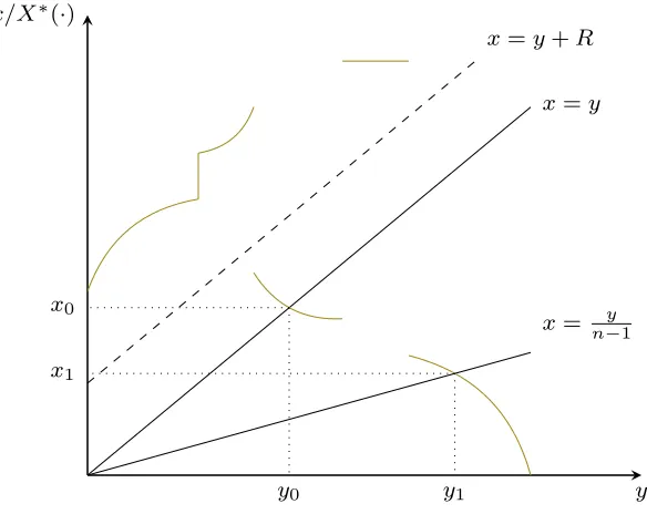
Figure 1 illustrates a typical best-response correspondence. Lemma 2
im-plies that every single-valued selection fromX∗must be decreasing (increasing)
in the the region below (above) the line x = y+R. This does not preclude
jumps in the best response back and forth between the two regions, but since
a symmetric equilibrium satisfies r(y∗) = ny−∗1 < y∗ +R, any symmetric
equi-librium occurs in the region, Φ1. Since the best response functions are all
decreasing in this region, and the line x= n−y1 is strictly increasing (in y), it
is clear that there is, at most, one point of intersection between the two. Lemma 2 is also useful for performing monotone comparative statics in our model. One can see from Figure 1 that an increase in the number of players
rotates the linex= n−y1 downwards. As a consequence, it is apparent that the
individual force in any symmetric equilibrium must decrease, while the joint
force of the other players must increase, following an increase in n. Our next
result formalizes this result, and also shows how payoffs change in response to a
change inn. In what follows, we letxtdenote the symmetric equilibrium force
when the parameter of interest is equal to t. Similarly, we let yt, zt, and πt
denote equilibrium others’ force, equilibrium total force, and the equilibrium per-player payoff, respectively.
Proposition 2. Suppose Assumption 1 is satisfied. For a fixed n ≥ 2, in a symmetric equilibrium, for n00 > n0,
(i) The individual force (and effort) is decreasing in the number of players: xn00 ≤xn0.
(ii) The other players’ joint force is increasing in the number of players: yn00 ≥yn0.
(iii) The expected per-player payoff is decreasing in the number of players: πn00 ≤πn0.
Consistent with other results that invoke lattice-theoretic techniques, our findings only ensure weak monotonicity of individual forces/efforts and
pay-offs in n. The following example shows that strict monotonicity cannot be
x=y
x= ny1
x=y+R
y x/X⇤(·)
y0
x0
y1
x1
[image:12.612.162.454.112.344.2]1
Figure 1: An example of a typical best-response correspondence (in green). Each selection from X∗ must be increasing in the region above the line x=y+R, and decreasing in the region below this line.
Example 1. Let φ(e) =e, V = 10, R = 0,5 and
C(e) =
√
e e≤1
(e+ 1)2−3 e≥1
For each n= 2, . . . ,10there exists a unique symmetric equilibrium in which all players choose e∗ =x∗ = 1.
We next study how symmetric equilibrium behavior depends on the other
parameters of the model, namely, the value of the prize, V, and the discount
rate,R. Before doing so, we introduce a new parameter that may be of interest
in some applications. Suppose that each player’s cost function depends on a
parameter,θ ∈R. Assume thatC is strictly submodular in (e, θ). That is, for
alle00> e0 and θ00> θ0 assume:
5The main idea in this example would also hold for R strictly positive but sufficiently
C(e00, θ00)−C(e0, θ00)< C(e00, θ0)−C(e0, θ0)
If C is twice differentiable in e and θ, then the condition above is implied
byC12<0 (equivalently,κ12 <0). That is, an increase in θ strictly decreases
the marginal cost of effort.
Proposition 3. Fix n≥ 2 and suppose Assumption 1 is satisfied. Then in a symmetric equilibrium,
(i) Individual and total forces/efforts are increasing in the value of the prize: For V00> V0, xV00 ≥xV0 and zV00 ≥zV0.
(ii) Individual and total forces/efforts are increasing in the cost parameter: For θ00 > θ0, xθ00 ≥xθ0 and zθ00 ≥zθ0.
(iii) Individual and total forces/efforts are decreasing in the discount rate: For R00 > R0, xR00 ≤xR0 and zR00 ≤zR0.
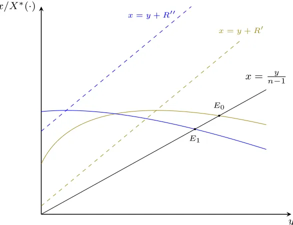
Parts (i) and (ii) of Proposition 3 follow from the fact that π is strictly
supermodular in (x, V) and (x, θ). By Topkis’ Theorem, an increase in either
of these parameters shifts a player’s best response upward, and leads to an increase in individual force/effort in any symmetric equilibrium. Figure 2
illustrates: Following an increase in V or θ, the player’s best response shifts
up from the green to the blue curve, and the symmetric equilibrium increases
from the point E0 to the point E1.
To understand part (iii) of Proposition 3, first note that π depends on R
and y insofar as it depends on the sum, y+R. Adapting Lemmas 1 and 2, it
is straightforward to show that, for any fixed y ≥ 0,π is strictly submodular
in (x, R) on Φ1, and that any selection, r(y), is decreasing in R whenever it
is contained in Φ1. So, suppose R increases from R0 to R00. When a player’s
best response correspondence is contained in Φ1 (for both parameter values),
this portion of the best response must shift down, following the increase in the parameter. Figure 3 illustrates; the green curve is the best response when
x= ny1
x=y+R
E1
E0
y x/X⇤(·)
[image:14.612.163.453.115.352.2]4
Figure 2: An illustration of the impact of an increase in V orθ on the best response corre-spondence. The green curve represents the best response before the parameter increase; the blue curve represents the best response after the parameter increase. Following the parameter change, the symmetric equilibrium increases fromE0 toE1.
the region between the lines, x = y+R0 and x = y+R00, the relationship
between the two best-response functions is difficult to ascertain in general. In
the region below the linex=y+R0, there is a clear ordering between the two,
with the best-response shifting down following the increase in the parameter. As any symmetric equilibrium occurs below this line, we can conclude that the symmetric equilibrium force decreases.
We now explore the relationship between the parameters of the model, and equilibrium payoffs. When the contest technology exhibits decreasing returns
to scale, Nti shows that equilibrium payoffs increase in V. The next example
shows that this result does not hold in general. Indeed, equilibrium per-player
payoffs may be strictly decreasing in the prize or the cost parameter, θ.
Example 2. Suppose n = 2, φ(e) = e, R = 0,6 and
6The main idea in this example would also hold for R strictly positive but sufficiently
x= ny1
x=y+R0 x=y+R00
E0
E1
y x/X⇤(·)
[image:15.612.160.453.114.339.2]2
Figure 3: An illustration of the impact of a change inRon the best response. The green curve is the best response when R =R0; the blue curve is the best response whenR =R00 > R0. Following an increase in R, the equilibrium decreases from E0 toE1.
C(e, θ) =
e
θ e≤1 eα
αθ + α−1
αθ e≥1
If 1≤ V θ4 ≤ 11−−2αα, the symmetric equilibrium per-player effort/force is
e∗ =x∗ =
V θ
4
α1
.
The equilibrium per-player payoff is
π∗ = 1−α
αθ −V
1−2α
4α
.
For 0 < α < 12, it is clear that π∗ is is strictly decreasing in V for fixed θ, and strictly decreasing in θ for fixedV. For instance, if α= 13 and θ = 1 then for 4 ≤ V ≤ 8, x∗ = V43
, and π∗ = 2− V4. If α = 13 and V = 1 then for
4≤θ≤8, e∗ =x∗ = θ43
There are two competing forces acting on a player’s equilibrium payoff fol-lowing an increase in the prize. First, is a direct positive effect, since the value of winning the contest increases. Second, there is an indirect negative effect, resulting from an increase in the efforts of one’s rivals. A priori, it is unclear which effect dominates. Nti shows that the direct positive effect outweighs the indirect negative effect when the contest technology exhibits decreasing returns to scale. For such technologies, the indirect effect is muted since higher levels of force are produced at greater marginal cost. For contest technologies with increasing returns to scale, a contrasting logic applies: Players’ optimal efforts are more sensitive to changes in the prize, and the indirect effect is
exacer-bated. This effect is evident in Example 2, as ∂2x∗
∂α∂V <0. That is, a decrease in
α, which leads to more pronounced increasing returns to scale, implies that x∗
is more sensitive to changes in the prize. As the example shows, with increas-ing returns it may well be that the indirect effect dominates the direct effect.
A similar intuition holds for changes inθ; as a result, the relationship between
equilibrium per-player payoffs and V/θ is ambiguous in general. But as our
next result shows, there is a clear relationship between the discount rate, R,
and equilibrium payoffs.
Proposition 4. Suppose Assumption 1 is satisfied. In a symmetric equilib-rium, the per-player expected payoff is decreasing in the discount rate: For R00> R0, πR0 ≥πR00.
As with an increase in V or θ, there are two competing forces acting on
equilibrium payoffs following a decrease inR. There is a direct positive effect,
since a decrease in R increases the likelihood of a player winning the prize.
But there is an indirect negative effect caused by the increase in the efforts of one’s rivals (see Proposition 3(iii)). As it happens, the positive effect always outweighs the negative effect. Indeed, the proof of Proposition 4 shows that,
following a decrease inR, although the efforts of one’s rivals increase, the sum
y+R decreases.
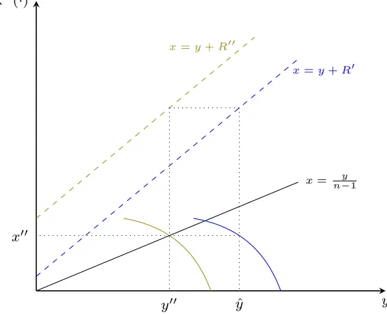
To understand why this result must hold in general, recall from the
it depends on y+R. Following a decrease in R from R00 to R0, a player’s
best-response shifts outward by a horizontal distance of R00− R0. Figure 4
illustrates: The green curve is (a portion of) the best response when R=R00,
and the blue curve is the best response whenR=R0 < R00. When the
parame-ter isR00, we see that equilibrium others’ total force isy00. At the point ˆy > y00,
it holds: ˆy+R0 = y00+R00. Since x00 is a best response to y00 when R = R00,
then x00 must also be a best response to ˆy when R =R0. Since any selection
from the best response (whenR =R0) is decreasing inybelow the blue dashed
line, any point of intersection between the blue best response curve and the
line x= n−y1 must occur at a valuey0 ∈[y00,yˆ]. This means y0+R0 ≤y00+R00.
Using this fact, it is straightforward to show that a player’s equilibrium payoff
must increase following a decrease in R.7
x= ny1
x=y+R00
x=y+R0
y x/X⇤(·)
x00
[image:17.612.175.452.340.565.2]y00 yˆ
Figure 4: An illustration of the impact of a change inR on (a portion of ) the best response correspondence. The green curve is the best-response when R =R00; the blue curve is the best response whenR=R0 < R00.
7Figure 4 illustrates a scenario in whichy+Rstrictly decreases in equilibrium following
Summarizing
The comparative statics results provided in Propositions 2 - 4 generalize results in Nti (1997), which assumes decreasing returns to scale, and utilizes first-order conditions. We have shown that neither decreasing returns to scale nor differentiability are essential drivers of these results. Rather, it is the structure implied by the ratio form CSF itself that drives the generic properties of the best response correspondence, which we established in Lemma 2. At the same
time, Example 2 shows that the assumption of decreasing returns to scale is
an important driver of the typical finding that equilibrium payoffs increase in the value of the prize.
3.2
Equilibrium Existence and Effects of Entry
We next turn to the question of existence, and study how aggregate behavior varies with the number of players. Our results in this section make use of the fact that the contest we study is equivalent to a symmetric Cournot oligopoly
with inverse demand, RV+Q, and cost function κ. Noting this equivalence, the
next results are consequences of our Proposition 1, and results in AL. We strengthen Assumption 1 as follows:
Assumption 2.
(i) For all e > 0, φ(e) is twice continuously differentiable with φ0(e) > 0. Moreover, φ(0) = 0.
(ii) For all e≥0, C(e) is twice continuously differentiable with C0(e)≥0.
We do not wish to rule out the widely-used Tullock CSF, which is not
differentiable at zero when r < 1. For this reason, we do not require φ(0) to
be differentiable; Assumption 2 is otherwise consistent with assumptions in AL.
Noting that z =x+y, a player’s payoff can be expressed as,
˜
π(z, y) = z−y
We can then think of some player i as choosing the total force, taking the
total force of the other players, as given. That is, player i solves,
max{π˜(z, y)|x+y≥z ≥y} (6)
We let Z∗(y) denote the argmax in (6), and let rz denote an arbitrary
single-valued selection from Z∗. Note that Assumption 2 ensures that κ(x) is
twice continuously differentiable for allx >0. For allz > y, let ∆(z, y) denote
the cross partial of ˜π with respect to z and y:
∆(z, y) = V
(R+z)2 +κ
00(z−y).
Note that ∆ is defined on the lattice,
Φ ={(z, y)∈R+|(n−1)x≥y≥0, y+x≥z > y}.
As in AL, the sign of ∆ on Φ plays a critical role in our analysis. When
∆ > 0 on Φ, ˜π is strictly supermodular in (z, y), which implies that any
selection fromZ∗ is increasing iny. Conversely, ∆<0 implies that ˜πis strictly
submodular in (z, y), which implies that any selection from Z∗ is decreasing
iny. First we consider the case where ∆>0 on Φ.
Proposition 5. In addition to Assumptions 1(iii) and 2, suppose ∆ > 0 on
Φ. Then,
(i) For each n ∈ N, there exists a unique symmetric equilibrium, and no asymmetric equilibria.
(ii) The equilibrium total force is increasing in n: For n00> n0, zn00 ≥zn0.
increasing in the number of players.8 Yet in some situations, comparisons in
total force are more meaningful than comparisons in total effort. Consider, for example, a contest designer interested in encouraging the development of a new technology. What is relevant is the probability with which at least one
player succeeds. This probability, Rz+z, depends only on the equilibrium total
force.
The key for Proposition 5 is the condition, ∆>0, which limits the returns
to scale of the contest technology, but also depends on the magnitudes of the discount rate and the prize. Jensen (2016) provides a result similar to Proposition 5 in an asymmetric contest under a different sufficient condition. In the special case where all players are symmetric, Jensen’s Assumption 3 amounts to,
C00 C0 ≥
φ00 φ0,
which is equivalent to convexity of κ. The condition, ∆ > 0, generalizes
Jensen’s result, for the case of a symmetric contest. To demonstrate this
generalization, note that ∆>0 ifκis convex, but as our next example shows,
∆ may be strictly positive, even ifκ is strictly concave everywhere.
Example 3. Suppose V = 1, R =.01, φ(e) =e, and
κ(x) =C(x) =x− 1
2(x+ 2) +
1 4
Note that κ00 <0 and,
∆(z, y) = 1
(z+.01)2 −
1
(z−y+ 2)3
It may be verified that for all y, π˜(z, y)<0 forz ≥1. So we may, without loss of generality, restrict attention to z ≤ 1. For all y ≤ z ≤ 1, it may be verified that ∆>0, and thus Proposition 5 applies immediately.
We now consider the case where ∆ < 0. Our next two results are
conse-quences of AL’s Theorems 2.5 and 2.6, respectively.
Proposition 6. In addition to Assumptions 1 and 2, suppose ∆ < 0 on Φ. Then, for any n∈N,
(i) For any m < n, if a symmetric equilibrium exists in the m-player con-test (with individual force xm, say) then the following configuration con-stitutes an equilibrium for the n player contest: Each of any m players chooses force xm while the remaining n −m players exert zero effort.
In particular, an n-player equilibrium always exists in which one player chooses the optimal single-player effort and the othern−1players choose zero effort.
(ii) A unique symmetric equilibrium exists if, for each y ∈ [0, y], π(·, y) is strictly quasiconcave.
(iii) No other equilibrium other than those described in parts (i) and (ii) can exist.
When ∆ < 0 over its domain, several asymmetric equilibria may exist;
moreover, there always exists an equilibrium in whichn−1 players are inactive.
An equilibrium with a single active player is not standard in contests. Note
that the condition, ∆ < 0 requires that R > 0. It should be clear that an
equilibrium with only one active player could never exist if R = 0. Note
moreover, that ∆<0 requires that the contest technology exhibits sufficiently
strong increasing returns to scale. The structure of equilibria is reminiscent of the structure found by Perez-Castrillo and Verdier (1992) and Cornes and Hartley (2005) under the Tullock CSF with increasing returns, and a discount
rate equal to zero.9 Although both of our results are driven by increasing
returns, neither is a special case of the other. This is most clearly illustrated
by noting that our result requires R > 0, while these other findings assume
R= 0.
Our next result shows how total equilibrium forces vary with the number
of players when ∆<0.
9Chowdhury and Sheremeta (2011) also show the potential for multiple asymmetric
Proposition 7. In addition to Assumptions 1 and 2, suppose ∆(z, y)<0 on
Φ. Then,
(i) Under the hypothesis of Proposition 6(i), all the asymmetric equilibria for all m < n are invariant in the number of players n.
(ii) Under the hypothesis of Proposition 6(ii), the total equilibrium force, zn,
is decreasing in n.
Proposition 7(i) clearly holds since, in the asymmetric equilibria with m <
n, an additional player exerts no effort. Proposition 7(ii) contrasts much of
the work in contests under the ratio form CSF.10Before discussing, we provide
an example illustrating this result.
Example 4. Let φ(x) =x, R= 3, V = 10, and
C(x) = κ(x) = 5 ln(x+ 2)− 5
x+ 3 −5 ln(2) +
5 3.
Note that
∆(z, y) = 10
(z+ 3)2 −
5
(z−y+ 2)2 −
10
(z−y+ 3)3
It may be verified that for all y, π˜(z, y)<0 for anyz ≥1.4. Then, without loss of generality, we can focus on the sign of ∆ when z ≤ 1.4. It may be verified that for all y ≤ z ≤ 1.4, ∆ < 0. There is a symmetric equilibrium with:
· n= 1: x1 =z1 ≈.618
· n= 2: x2 ≈.2068, z2 ≈.4137
· n= 3: x3 ≈.1188, z3 ≈.3565
· n= 4: x4 ≈.083, z4 ≈.332
10One exception is Amegashie (1999). Under the lottery CSF, Amegashie shows that
· n= 5: x5 ≈.0637, z5 ≈.3186
In addition to the symmetric equilibrium, there are multiple asymmetric equilibria, where, for any n, one player chooses x1, and the others exert no effort, another where 2 players choose x2 and the others choose zero, etc.
When ∆ < 0, it can be shown that a player’s best response, X∗, is fully
contained in Φ1 for all y. That is, R is sufficiently large, relative to the prize,
that for any y ≥ 0, x ∈ X∗(y) implies x < y+R. By Lemma 2 this means
that each selectionr(·) fromX∗ is decreasing for ally. In fact, it can be shown
that the best response functions are allstrictly decreasing (when interior), and
that an increase in y leads a player to reduce her force by so much that the
total force decreases. To understand why, recall that ∆<0 implies that any
selection,rz fromZ∗ is decreasing. For anyyit holdsrz(y) =r(y) +y, wherer
is some selection fromX∗. Sincerz is decreasing, this implies that the slope of
r is bounded from above by −1. Then, in a symmetric equilibrium, we know
by Proposition 2 that an increase in the number of players leads to an increase
in the total force of one’s rivals. Since total force is decreasing in y, it follows
that an increase inn leads to a decrease in symmetric equilibrium total force.
Proposition 7 implies that, when ∆<0, a contest designer could maximize
total force by excluding all but one player from the contest. It is worth relat-ing this findrelat-ing to the well-known Exclusion Principal of Baye et al. (1993). Baye et al. show that in an asymmetric contest under the all-pay auction
CSF,11 a contest designer can increase total effort by excluding the player
with the highest value. Intuitively, there is a “discouragement effect” whereby the presence of a high-value player discourages other players from exerting ef-fort. Removing the high-value player “levels the playing field”, and encourages greater effort among the remaining players (enough to offset the effort of the removed player). The choice of CSF plays a critical role in driving the Exclu-sion Principle. For instance, when marginal cost is constant, it is well-known
that the result does not hold under the Tullock CSF.12Intuitively, the Tullock
11Under the all-pay auction CSF, a player wins the contest with certainty if her effort is
greater than every other player’s effort.
CSF induces a softer form of competition than the all-pay auction CSF, and
the discouragement effect is less pronounced.13 In contrast to the Exclusion
Principal, our result applies in a symmetric contest. Rather than being driven by a leveling-the-playing-field idea, our result is driven by increasing returns to scale in the production of effort. Reminiscent of a natural monopoly in industrial organization, restricting the contest to a single player allows this player to take full advantage of her increasing returns to scale.
3.3
The case, R = 0
Since much of the work in the contest literature utilizing the ratio form CSF
assumes R = 0, in this section we explicitly address this case. Note that if
R = 0 and φ(0) = 0 then the ratio-form CSF is not well defined when ei = 0
for all i. We follow much of the literature and assume that if all players exert
zero effort, then each player wins with probability 1
n. Although most of our
results carry over to the case where R = 0, the uniqueness of a symmetric
equilibrium cannot be guaranteed. The following example illustrates:
Example 5. Let φ(e) =e, n = 2, V = 5, R = 0, and
C(e) =
e e≤ 12
2 + 4(e−92)3 1
2 ≤e ≤2
e e≥2
There are two symmetric equilibria; one equilibrium in which e∗ =x∗ = 1 2, and another in which e∗ =x∗ = 2.
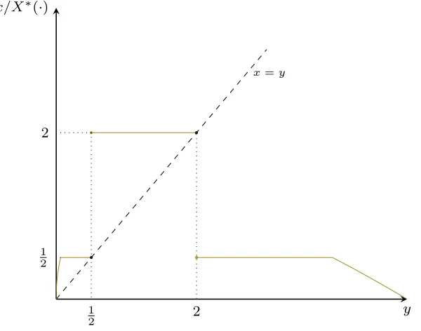
Example 5 demonstrates that when R = 0, multiple symmetric equilibria
may exist. Figure 5 illustrates the best-response correspondence for a player in this example. There are a couple features worth mentioning. First, is the
fact that there are exactly two players. When n = 2, the lines x = y +R
13Matros and Rietzke (2017) show that an exclusion result along the lines of Baye et al.
and x= n−y1 coincide. The best response functions are therefore increasing in
the region above the line, x = n−y1 =y, and decreasing below this line. Thus,
R = 0 and n = 2 represents a knife-edge case in which the best-response
functions are not decreasing in the relevant region where symmetric equilibria
occur, as is the case when R >0 or n >2. The second critical feature in this
example is the fact that κ is not everywhere differentiable. Our next result
highlights the relevance of these features.
x=y
y x/X⇤(·)
2
1 2 1
2
2
[image:25.612.161.461.244.480.2]1
Figure 5: The best-response correspondence (in green) for a player in Example 5.
Proposition 8. Suppose Assumption 1 is satisfied andR = 0. Then there ex-ist at most two symmetric equilibria. Moreover, if n ≥3or κ is differentiable, then there exists at most one symmetric equilibrium.
Proposition 8 shows that when R = 0, the contest possesses as most two
distinct symmetric equilibria, but if n > 2 or κ is differentiable, then any
symmetric equilibrium is unique. To understand this result, first note that for
n >2, the line x = n−y1 lies in the region Φ1. In this case, selections from the
best response are decreasing in the relevant region where any symmetric
is differentiable, it can be shown that every selection from the best response is
strictly decreasing when it is contained in Φ1 and strictly increasing when
con-tained in Φ2. Clearly, this rules out a best response along the lines of Figure 5.
More generally, it can be shown that, whenever multiple symmetric equilibria
exist when n = 2, the best response must be constant over some interval in
Φ1; differentiability rules out this possibility.
Our final result shows that, although the uniqueness of a symmetric
equi-librium cannot be guaranteed when R = 0, most of our other comparative
statics results continue to hold.
Proposition 9. In the model with R = 0, the statements of Lemmas 1-2, and Proposition 5 hold. Moreover, the statements of Propositions 2-4 hold, when one replaces “in a symmetric equilibrium” with “in the smallest and largest symmetric equilibria”.
As discussed in Section 3.2, R > 0 is a necessary condition for ∆ < 0 on
Φ; Propositions 6-7 are therefore excluded from the statement of Proposition 9. Aside from these results, our other comparative statics findings carry over
to the case where R= 0.
Tullock CSF
It is worth relating our findings in Section 3.2 to the commonly used Tullock
CSF, where φ(e) = er, and R = 0. For this CSF, it holds κ(x) = x1r, and ∆
becomes:
∆(z, y) = V
z2 +
1
r
1
r −1
(z−y)1r−2
It can be shown that ∆ >0 on its domain if and only if r ≤1. For r≤1,
Propositions 5/9 then imply that there exists a unique symmetric equilibrium,
and no asymmetric equilibria, for any n. Perez-Castrillo and Verdier (1992)
show that for anyr >1, asymmetric equilibria exist whennis sufficiently large
(specifically, n > r−r1). Thus, although ∆ >0 is, in general, only a sufficient
4
Conclusion
In this paper, we established a number of robust comparative statics results in a contest under the ratio-form CSF with minimal restrictions on the primi-tives. We furthermore shed new light on the issues of equilibrium existence and uniqueness. Our results help to clarify the relevance of the structure typically imposed in this model. The main innovation of this paper is the application of lattice-theoretic techniques, which have not previously been applied in con-tests. Utilizing these tools, we established a strong regularity condition on the shape of a player’s best response correspondence, out of which our compara-tive statics results follow. Our approach sheds light on how lattice-theoretic techniques can be applied in contests, which should help guide future research in developing more robust conclusions.
5
Appendix
Proof of Lemma 1
Letx00> x0 ≥xandy00> y0 ≥0. Let ˜y00 =y00+R and ˜y0 =y0+R. The reader can easily verify that expression (2) is equivalent to
x00 x00+ ˜y00 −
x00
x00+ ˜y0 <[>]
x0 x0+ ˜y00 −
x0 x0 + ˜y0,
which holds if and only if x00x0 <[>]˜y00y˜0.
Proof of Lemma 2
We will show the first statement in the lemma; the proof of the second
state-ment is analogous. Let y00 > y0 ≥ 0, x00 ∈ X∗(y00) and x0 ∈ X∗(y0). Suppose
x00x0 <(y00+R)(y0+R). Proceed by contradiction: Suppose, contrary to the
lemma,x00 > x0. Then by Lemma 1,
where the l.h.s. inequality follows sincex00 ∈X∗(y00), and the r.h.s. inequality
follows since x0 ∈ X∗(y0).14 We have a contradiction; hence it must be that
x00 ≤x0.
Proof of Proposition 1
Fixn≥2. We show that if a symmetric equilibrium exists, it must be unique.
Letx1andx2be two symmetric equilibrium levels of force, and let letyi = (n−
1)xi,i= 1,2. Proceed by contradiction, and suppose that these two equilibria
are distinct; in particular, suppose x1 > x2; equivalently, y1 > y2. Note that
for i = 1,2, xi and yi satisfy: xi ∈X∗(yi) and xi = ny−i1. But since ny−i1 ≤yi,
it must hold that xi < yi +R for i = 1,2; hence, x1x2 < (y1+R)(y2+R).
Since y1 > y2 (by assumption), Lemma 2 implies x1 ≤ x2, which yields a
contradiction. Therefore, the symmetric equilibrium must be unique.
Proof of Proposition 2
Parts (i)-(ii)
Fix n00 > n0, and suppose that a symmetric pure-strategy equilibrium exists
in the n00 and n0 player contests. From the arguments in the first part of this
proof, we know that the symmetric equilibrium must be unique. Let x00 (x0)
denote the individual equilibrium individual force when the contest has n00
(respectively, n0) players; let y00= (n00−1)x00 and y0 = (n0−1)x0.
We first show part (ii). First note that if y0 ≤(n00−1)x, then as feasibility
requires y00 ≥(n00−1)x, it follows that y00 ≥y0. Then supposey0 >(n00−1)x.
We will show that there cannot be a symmetric equilibrium withy < y0 when
n =n00. Fix y0 ∈[(n00−1)x, y0), and let x0 ∈X∗(y0). Clearly if x0 ≥ y0 +R
then x0 > n00y−01. If x0 < y0 +R, then Lemma 2 implies x0 ≥ x0. But since n00 > n0 and y0 > y0 it holds, x0 = y
0
n0−1 > y 0
n00−1 > n00y0−1; thus, x0 > n00y−01.
We have now established that for all y ∈ [(n00 −1)x, y0), x ∈ X∗(y) implies
x > n00y−1; thus, there cannot be a symmetric equilibrium with y < y0 when
n=n00. It follows that y00≥y0. This establishes part (ii).
14The choice set, [x, x], is independent ofy, so x0 (x00) is certainly feasible when others’
Next, we show x00 ≤ x0. We have already shown that y00 ≥ y0. If y00 = y0
thenn00> n0, impliesx00= n00y00−1 < n0y0
−1 =x0. Ify00 > y0 then since x00< y00+R
and x0 < y0 +R, Lemma 2 implies x00 ≤ x0. Since individual force decreases
following the increase in n, clearly individual effort decreases as well. This
establishes part (i).
Part (iii)
Let π00 (π0) denote the equilibrium individual expected payoff in the contest
with n00 (respectively, n0) players where n00> n0. We have the following string
of inequalities:
π0 = x0
R+x0+y0V −κ(x 0)
≥ x00
R+x0+y0V −κ(x 00)
≥ x
00
R+x00+y00V −κ(x 00)
=π00
The first inequality holds by definition ofx0. The second inequality follows
since, as we showed in part (ii), y00 ≥ y0. This establishes part (iii) and the
proposition.
Proof of Proposition 3
We prove parts (i) and (ii) jointly. Fixn, and lettdenote either the parameter
V or θ. It is easily verified that π is strictly supermodular in t and x. By
Topkis’ Theorem (see, e.g. Topkis, 1978, or Theorem A.1 in AL), it follows
that any selection, r(·), from X∗ is increasing in t for each y. It is clear that
this implies that any intersection between a player’s reaction curve and the
line x= n−y1 must lie further from the origin following an increase in t. Since
individual force increases, then individual effort and total force/effort must
increase, as n is fixed. This proves parts (i) and (iii).
equilib-rium exists for both parameter values. Let x00 and x0 denote the symmetric
equilibrium individual force when the parameter is R00, respectively R0. Let
y00 = (n−1)x00 and y0 = (n−1)x0. Since π depends on y and R insofar as it
depends on the sum,y+R,X∗ depends only on this sum. We writeX∗(y+R)
to denote the set of best-replies toy when the parameter is R. Note that our
result follows immediately if x00=x; so, assume x00> x; equivalently, y00> y.
Let ˆy=R00−R0+y00 > y00. By construction, ˆy+R0 =y00+R00; therefore,
X∗(ˆy+R0) = X∗(y00+R00). By definition ofx00, this meansx00∈X∗(ˆy+R0). We
now show that there cannot be a symmetric equilibrium in whichy < y00 when
R = R0. Fix y0 ∈ [y, y00), and let x0 ∈ X∗(y0 +R0). Clearly, if x0 > y0+R0
then x0 > y0
n−1. If x0 ≤ y0 + R0, then since x00 ≤ y00 < yˆ+R0, it holds
x0x00 < (y0 +R0)(ˆy +R0). As, x0 ∈ X∗(y0 + R0), x00 ∈ X∗(ˆy +R0), and
ˆ
y > y00 > y0, Lemma 2 implies x0 ≥x00= y
00
n−1 >
y0
n−1.
We have now shown that for ally∈[y, y00),x∈X∗(y+R0) impliesx > n−y1;
thus, there cannot exist a symmetric equilibrium in whichy < y00whenR =R0.
It therefore must be thaty0 ≥y00; equivalently, x0 ≥x00. Since individual force
increases following a decrease inR, then individual effort and total force/effort
must increase, asn is fixed. This establishes part (iii) and the proposition.
Proof of Proposition 4
Let R00 > R0 and suppose that a symmetric equilibrium exists for both
pa-rameter values. Let x00 (x0) denote the equilibrium per-player force when the
parameter is R00 (R0). Let y00 = (n−1)x00 and y0 = (n−1)x0. Finally, let
X∗(y+R) denote the best response to y when the parameter isR.15
Let ˆy=y00+R00−R0 > y00. As we showed in the proof of Proposition 3(ii),
it must be that x00 ∈ X∗(ˆy+R0). Moreover, since x00 = ny−001 < n−yˆ1 <yˆ+R0,
Lemma 2 implies that for all y > yˆ, if x ∈ X∗(y+R0) and x < y +R0, then
x ≤x00 < ny
−1. Thus, there cannot exist a symmetric equilibrium with y > yˆ
when R = R0. Therefore, y0 ≤ yˆ, which implies y0 +R0 ≤ yˆ+R0 = y00+R00.
Next, letπ00 (π0) denote the equilibrium payoff to a player when the parameter
15Recall from the proof of Proposition 3(ii) that a player’s best response depends on y
is R00 (respectively, R0). It holds,
π0 = x
0
x0+y0+R0V −κ(x 0)
≥ x
00
x00+y0+R0V −κ(x 00)
≥ x
00
x00+y00+R00V −κ(x 00)
=π00
The first inequality follows by definition of x0; the second follows since
y00+R00 ≥y0+R0. This establishes the proposition.
Proof of Propositions 5-7
The contest is equivalent to a symmetric Cournot oligopoly with inverse
de-mand function ˜P(z) = RV+z, and cost function, ˜C(x) = κ(x). The existence of
a symmetric equilibrium, and non-existence of any asymmetric equilibria es-tablished in Proposition 5 follows from Theorem 2.1 in AL. The uniqueness of this equilibrium follows from Proposition 1. Part (ii) of Proposition 5 follows immediately by Theorem 2.2(b) in AL. Propositions 6 and 7 follow by AL’s Theorems 2.5 and 2.6, respectively.
Proof of Proposition 8
We first show that if n ≥3 or κis differentiable, then any symmetric
equilib-rium must be unique. First note that Lemmas 1 and 2 immediately generalize
to the case R = 0. If n ≥ 3 then in any symmetric equilibrium it holds,
x∗ = ny−∗1 < y∗ +R = y∗. Using this fact, the proof of Proposition 1 applies
immediately to the case R = 0. Then suppose n = 2 and κ is differentiable.
Proceed by contradiction, and suppose there exist at least two distinct
sym-metric equilibria with individual forces x00 > x0. Let y00 and y0 denote the
clarity, we use different notation to denote the other player’s action). Now, it may easily be verified that,
π(x00, y00)−π(x0, y00) =π(x00, y0)−π(x0, y0)
Since x00 ∈X∗(y00) and x0 ∈X∗(y0) it holds,
0≤π(x00, y00)−π(x0, y00) = π(x00, y0)−π(x0, y0)≤0.
Thus, the two inequalities must hold with equality. Therefore, π(x00, y00) =
π(x0, y00) and π(x00, y0) = π(x0, y0), which meansx00 ∈X∗(y0) and x0 ∈X∗(y00).
Now, since κ is differentiable, this implies π is differentiable in x for each
y >0. Sincey00> y0 ≥0, π(·, y00) is differentiable. Also note thatx00 > x0 ≥x
means thatx00 is interior. Sincex00 ∈X∗(y0) andx00 ∈X∗(y00) this implies that
x00 must satisfy the following first order conditions:
y0
(x00+y0)2V −κ
0(x00) = y00
(x00+y00)2V −κ
0(x00) = 0
which means,
y0
(x00+y0)2 =
y00
(x00+y00)2 (7)
Let Γ(y) = (x00+yy)2. Note that for all y∈[y0, y00) it holds, Γ0(y) =
x00−y
(x00+y)3 >
0. This implies Γ(y00)>Γ(y0), which contradicts (7). Thus, ifκis differentiable
and a symmetric equilibrium exists, it must be unique.
We now complete the proof of the proposition by showing that there can
exist at most two symmetric equilibria. We have already shown that ifn ≥3
then the contest possesses at most one symmetric equilibrium. So, the only
relevant case to address is for n = 2. We proceed by contradiction: Suppose
there exist at least three distinct symmetric equilibria. Choose any three of
these equilibria; let x0 denote the smallest individual force of these three, and
let x00 > x0 denote the largest individual force of these three. Let y00 > y0
represent the corresponding forces of the other player.
there must be a point, y0 ∈ (y0, y00) such that y0 = x0 ∈X∗(y0). Recall from
the first part of this proof that x00 ∈ X∗(y0). Since x00 > y0 and x0 = y0, it
holds,x00x0 > y0y0. Asy0 > y0, Lemma 2 impliesx0 ≥x00; equivalentlyy0 ≥y00,
which yields a contradiction. Our hypothesis that there exist at least three distinct symmetric equilibria leads to a contradiction, and thus there can exist at most two.
Proof of Proposition 9
The fact that Lemmas 1-2 extend in this case is immediate. The proofs for
Propositions 2-4 are also nearly identical whenR = 0, so we do not reproduce
these here. The only issue in applying the result of AL for Proposition 5 is that
π is discontinuous at the zero vector when x=R = 0. However, Assumption
2 implies that π is continuous in x for any y > 0. In particular, this means
that X∗(y) is non-empty for any y >0. Since, in any symmetric equilibrium,
all players must exert strictly positive effort when x =R = 0, the arguments
made by AL can easily be adapted to deal with this point of discontinuity. We therefore do not reproduce the proof here.
References
Acemoglu, D. and Jensen, M. K. (2013). Aggregate comparative statics.
Games and Economic Behavior, 81:27–49.
Amegashie, J. A. (1999). The number of seekers and aggregate
rent-seeking expenditures: an unpleasant result. Public Choice, 99(1):57–62.
Amir, R. (1996). Cournot Oligopoly and the Theory of Supermodular Games.
Games and Economic Behavior, 15(2):132–148.
Amir, R. (2005). Supermodularity and Complementarity in Economics: An
Elementary Survey. Southern Economic Journal, 71(3):636–660.
Amir, R. and Lambson, V. (2000). On the effects of entry in Cournot markets.
Baye, M. R., Kovenock, D., and De Vries, C. G. (1993). Rigging the lobbying
process: An application of the all-pay auction. The American Economic
Review, 83(1):289–294.
Chowdhury, S. M. and Sheremeta, R. M. (2011). Multiple equilibria in Tullock
contests. Economics Letters, 112(2):216–219.
Corch´on, L. C. (2007). The theory of contests: A survey. Review of Economic
Design, 11(2):69–100.
Cornes, R. and Hartley, R. (2005). Asymmetric contests with general
tech-nologies. Economic Theory, 26(4):923–946.
Fang, H. (2002). Lottery versus all-pay auction models of lobbying. Public
Choice, 112(3-4):351–371.
Jensen, M. K. (2016). Existence, uniqueness, and comparative statics in
con-tests. In Equilibrium Theory for Cournot Oligopolies and Related Games,
pages 233–244. Springer.
Konrad, K. (2009). Strategy and Dynamics in Contests. Oxford University
Press, New York, NY.
Loury, G. C. (1979). Market structure and innovation. The Quarterly Journal
of Economics, pages 395–410.
Matros, A. (2006). Rent-seeking with asymmetric valuations: Addition or
deletion of a player. Public Choice, 129(3-4):369–380.
Matros, A. and Rietzke, D. (2017). Contests on networks. Lancaster University Management School Working Paper Series 2017/006.
Menicucci, D. (2006). Banning bidders from all-pay auctions. Economic
The-ory, 29(1):89–94.
Milgrom, P. and Roberts, J. (1994). Comparing equilibria. The American
Milgrom, P. and Shannon, C. (1994). Monotone comparative statics. Econo-metrica, 62(1):157.
Nti, K. O. (1997). Comparative statics of contests and rent-seeking games.
International Economic Review, 38(1):43–59.
Perez-Castrillo, J. D. and Verdier, T. (1992). A general analysis of rent-seeking
games. Public Choice, 73(3):335–350.
Skaperdas, S. (1996). Contest success functions. Economic Theory, 7(2):283–
290.
Szidarovszky, F. and Okuguchi, K. (1997). On the existence and uniqueness
of pure Nash equilibrium in rent-seeking games. Games and Economic
Be-havior, 18(1):135–140.
Topkis, D. (1978). Minimizing a submodular function on a lattice. Operations
Research, 26(2):305–321.
Topkis, D. M. (1998). Supermodularity and complementarity. Princeton
uni-versity press.
Tullock, G. (1980). Efficient rent-seeking. In Buchanan, J. M., Tollison, R. D.,
and Tullock, G., editors, Toward a theory of the rent-seeking society,
num-ber 4, pages 97–112. Texas A&M University Press, College Station, Texas.
Vives, X. (1990). Nash equilibrium with strategic complementarities. Journal
of Mathematical Economics, 19(3):305–321.
Yamakazi, T. (2008). On the existence and uniqueness of pure-strategy nash
equilibrium in asymmetric rent-seeking contests.Journal of Public Economic