Microstructural Modeling and Thermal Property Simulation of Unidirectional Composite

Microstructural Modeling and Thermal Property

Simulation of Unidirectional Composite

Keiko Kikuchi

, Yan-Sheng Kang

, Akira Kawasaki

, Shinya Nishida

and Akira Ichida

1

Department of Materials Processing, Graduate School of Engineering, Tohoku University, Sendai 980-8579, Japan 2_{A.L.M.T. Corp., Toyama 931-8543, Japan}

The electrical, thermal and mechanical properties of functionally graded materials vary with microstructure and composition. Consequently it is very important to know quantitatively the properties of composites for the design of functionally graded materials. However, few methods of quantitative and theoretical evaluation for material properties on wide compositional range have been established. In this research, a method that estimates the material properties of composites directly from their microstructure assisted with finite element analysis was investigated. As an example of the estimation of material properties, the thermal conductivity of Mo fiber-Cu matrix composites has been evaluated. Calculated results of thermal conductivity are well in agreement with the experimental data measured by using a laser flash apparatus and the smallest deviation is 1.9%. The finite element analysis using a metallographic model is a very accurate method for estimation of composite properties.

(Received September 26, 2003; Accepted December 15, 2003)

Keywords: microstructural modeling, thermal conductivity, unidirectional composite, copper-molybdenum composite

1. Introduction

Recent technological advancement requires advanced materials with multiple superior properties suited for each application.1–4) Functionally graded materials in which internal properties vary continuously with the change of their microstructure and composition5,6)have the potential to meet such requirements. In order to fabricate the functionally graded materials having desired functions, determination of optimal components and spatial distribution of composition is necessary based on quantitative estimation of material properties. However, numerous combinations of materials and their compositions cause considerable efforts and time for the optimization. Hence, some numerical and analytical methods for quantitative estimation of material properties become very important for designing the functionally graded materials. Many analytical approaches for the quantitative evaluation of material properties of composites are found in literatures,7–9) most of them, however, involve several restrictions on the morphology of the microstructures. This is due to insufficient information about the microstructural geometry or the incapability of dealing with the geometrical complexity in numerical modeling of the actual micro-structures which are generally very complicated. Therefore, there may be potential errors in estimating the effective material properties by means of analytical methods.

Hollister and Kikuchi10) _{reported a numerical method}

which allows the determination of appropriate microstruc-tural geometry models. They extensively utilized digital images of the microstructure so that their processing technique is called Digital Image Based (DIB) modeling. The technique is used to construct the digitalized Finite Element (FE) model of a bone microstructure by identifying each voxel as a finite element. Along with the asymptotic homogenization method, their DIB modeling technique enabled the quantitative study of the macro- and micro-mechanical characteristics of bone’s porous skeleton in the framework of linear elasticity.

Another method which enables the estimation of material properties of composites directly from the actual micro-structure assisted with DIB technique and finite element analysis was proposed in our previous work.11) In this method, the material properties are estimated directly from the results of finite element analysis. Hence, not only mechanical, thermal, and electrical properties but also combined properties (e.g. thermal expansion and piezo-electric properties) are evaluated by just providing the suitable boundary conditions for the model. In addition, the local distribution of material properties in the case of functionally graded materials could also be evaluated by this method since it does not necessarily require the assumption of local periodicity of the media. Therefore, this method offers very high potential for the optimization and evaluation of functionally graded materials, and becomes an addition to the very few methods established for quantitative evaluation. However, the accuracy of material properties estimated by this method has not been evaluated.

The purpose of this paper is to reveal the estimation accuracy of the method assisted with DIB technique and finite element analysis on the thermal conductivity of a composite. A Mo fiber-Cu matrix composite prepared through the infiltration process was selected as a target material. In this case, the composite was a unidirectional composite and 2-dimensional analytical model was easily taken into account because the arrangement of circular Mo phase was observed in the plane perpendicular to the axis of the Mo fiber. Then, the thermal conductivities of the composite were estimated in 2-dimensional analysis. The estimated thermal conductivities have been compared with both of those calculated by the theories and experimental results obtained by laser flash method.

2. Analysis and Experiment Procedure

2.1 Microstructural modeling for composites

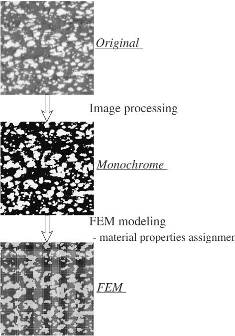
this paper is shown in Fig. 1. Digital Image Based (DIB) geometric modeling technique10,12) _{was used to reflect the}

actual morphology of composite microstructure such as inclusion shape, volume fractions, etc. on Finite Element (FE) model. The DIB technique for 2-dimensional models can be divided into three parts. First, the image of composite microstructure observed by optical micrograph, SEM, EPMA and so on, is captured as a digital image by an optical sensor. The second step contains the image processing which emphasizes the contrast of colors (e.g. thresholding) con-ducted to the digitalized microstructure in order to separate it into a domain of each component. As for the third step, the processed image is converted into FE model by recognizing each pixel in images as a 4-node square finite element, that is, each same size finite element has the material constants of a component according to the value of the corresponding pixel. This DIB technique has a great advantage of excluding any meshing manipulation such as defining coordinates and element connectivities because all the elements have the same size.

2.2 Estimation of thermal conductivity

In this work, the material property of composite was estimated assisted with Finite Element Analysis (FEA). The FE model described in previous section was applied suitable boundary conditions and subsequently analyzed by FEA. The effective property of the model was calculated from the results of FEA using the basic laws in physics. In the case of

estimation of thermal conductivities, the FE model was applied boundary conditions as shown in Fig. 2; an arbitrary uniform difference of temperatureT, between distanced, of the surfaces in the direction of estimation and periodical condition on the rest of the surfaces. In this paper, theT

was determined as 10 K. The average heat flux, Q, was obtained subsequently using FEA and the effective thermal conductivity, eff, of the model was determined by the

following expression,

eff¼QT=d: ð1Þ

2.3 Fabrication and evaluation of Mo fiber-Cu matrix composite

Mo fiber-Cu matrix composite specimens were prepared from Mo fibers with a diameter of 120mmand Cu plates. The Mo fibers were electrolyzed, cleaned and straightened. Then about 5000 fibers were bundled in a diameter of 10 mm. The molten Cu was then infiltrated into the bundle of Mo fibers in hydrogen atmosphere. This infiltration was performed in a graphite crucible for 60 seconds at 1503 K then cooled in a furnace.

Thermal diffusivity was measured using laser flash technique (Netzsch, LFA-427) at room temperature. The specimens were in the form of 10 mm-diameter circular disks with a thickness of 1 mm. Density of the specimens was measured by Archimedes’ method, and composition of the specimens was determined from the measured density assuming that the specimens were fully densified. Specific heat was obtained as the weight percentage of the specific heat of each constituent.13) _{Thermal conductivity was}

calculated as a product of thermal diffusivity, specific heat, and density of the specimens. Microstructures of the speci-mens were observed by optical microscope and scanning electron microscope (SEM).

3. Thermal Conductivities of the Ideal Model for Unidirectional Composite

3.1 Modeling of ideal microstructure

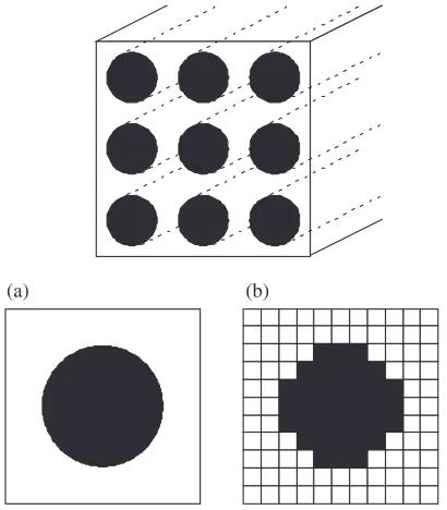
The model of unidirectional circular cylinders packed in square arrays is shown as an ideal unidirectional composite in Fig. 3. From this ideal model, it is assumed that (a) the composites are macroscopically homogeneous, (b) locally,

Monochrome

Original

FEM modeling

- material properties assignment

FEM

Image processing

Fig. 1 Procedure for microstructural modeling.

Temperature Difference

∆

T=10K

Periodical Condition

both the matrix and the fiber are homogeneous and isotropic, (c) the thermal contact resistance between the fiber and matrix is negligible, (d) the problem is two-dimensional, and (e) the fibers are arranged in a square periodic array,i.e.they are uniformly distributed in the matrix. The model shown in Fig. 3(a) is a unit cell which represents one-cycle of the periodic structure, so the transverse thermal conductivity of unidirectional composite of circular cylinders was estimated by using this unit cell. The unit cell was divided into 4-node fixed size square elements as shown in Fig. 3(b), so that the FE model obtained from the unit cell became equivalent to that obtained from the microstructure of composites. Under the conditions described above, the microstructure is re-stricted to the model size in the direction of estimation even though it is assumed to spread infinitely in other directions. So, the models which consist of several unit cells as shown in Fig. 4 are considered in this work for evaluating the effect of boundary conditions. When the model consists of several unit cells, multiplying the number of elements per unit cell by the number of unit cells gives the total number of elements in the model. Thus, the number of unit cells represents the size of the model in this study. The analysis conditions are shown in Table 1.

3.2 Justification of modeling

The effects of the analysis conditions shown in Table 1 on thermal conductivities estimated from the microstructure are evaluated in this section.

Figure 5 shows the relationship between the estimated thermal conductivity and the number of elements for 4 different ratios of f=m, where, f is the fiber thermal

conductivity andmis the matrix thermal conductivity. There

is one unit cell for the model. The estimated thermal conductivity becomes close to a certain value where the number of elements per unit cell is over 3000. Each standard deviation for four points surrounded by dashed line in Fig. 5 is under 1%. The boundary in FE model made in the DIB technique has zigzag shapes, different from the real micro-structure, because the model consists of assembly of fixed sized square elements. These results indicate that if the number of elements in the model is large enough to represent the accurate geometry of microstructures, the thermal conductivity of composites can be accurately evaluated from their microstructure. The number of unit cells must be as large as possible to have a more accurate result. However, when the number of elements is larger, the larger memory size of a computer is also required. In the case of composites of unidirectional circular cylinders packed in square arrays, the 3000 elements per unit cell can be assumed to be large enough to estimate the thermal conductivity accurately.

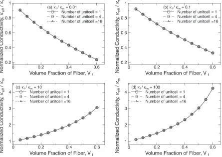
Figure 6 shows the thermal conductivities estimated by the models, those of different number of unit cells for 4 different ratios of f=m. Each model was divided into 10201

elements per unit cell. The standard deviations for three results of the same composition were approximately104_%, respectively. These results indicate that in the case of composites of unidirectional circular cylinders packed in square arrays, the number of unit cells in the model does not influence on the estimated thermal conductivity. That is, the estimated thermal conductivity is not affected by the boundary conditions described in previous section which restricts the model size. Hence, the thermal conductivity is estimated accurately enough by analysis on one unit cell. Hereafter, the estimation of thermal conductivity described in this study is done by the model consisting of only one unit cell.

3.3 Comparison with the established theories

A large number of theories are available for predicting the transverse thermal conductivity of unidirectional composites. Out of the many predictive models for transverse thermal conductivity of unidirectional composites, the models of Chawla,14) Sprinter-Tsai,15) Hashin8) and Rayleigh16) were selected as representative examples of circular cylinders packed in square arrays. Also, the macroscopic heat transfer in periodic composites has been studied using the homoge-nization method.17,18) _{The estimation method for material}

(a) (b)

Fig. 3 The schematic illustration of the unidirectional model for circular

cylinders packed in square arrays. (a) a unit cell. (b) the schematic illustration of FE model based on unit cell (a).

Fig. 4 An example of a model consisting of several unit cells.

Table 1 Analysis conditions.

Number of unit cell (Ne) 116

Number of element per unit cell 12114641

Ratio of thermal conductivity (f=m) 0:01100

Elements Number per Unitcell, N_e

Nor

m

aliz

ed Conductivity

,

κeff

/

κm

(b) κ_f/κ_m=0.1 V_f=0.3

100 1000 10000

0.58 0.59 0.6 0.61 0.62

Elements Number per Unitcell, N_e

Nor

maliz

ed Conductivity

,

κeff

/

κm

(a) κ_f/κ_m=0.01 V_f=0.3

100 1000 10000

0.51 0.52 0.53 0.54 0.55 0.56 0.57

Elements Number per Unitcell, N_e

Nor

maliz

ed Conductivity

,

κeff

/

κm

(d) κ_f/κ_m=100 V_f=0.3

100 1000 10000

1.9 2

Elements Number per Unitcell, N_e

Nor

maliz

ed Conductivity

,

κeff

/

κm

(c) κ_f/κ_m=10 V_f=0.3

100 1000 10000

1.7 1.8

Fig. 5 The estimated thermal conductivity for square array of cylinders as a function of the number of elements per unit cell for the

different ratio of thermal conductivity. The volume fraction of cylinder is 0.3 and the number of unit cell is 1.

(d) κ_f / κ_m = 100

Number of unitcell = 1 Number of unitcell = 4 Number of unitcell =16

Volume Fraction of Fiber, V_f

Nor

m

aliz

ed Conductivity

,

κeff

/

κm

0 0.2 0.4 0.6

1 2 3 4

(c) κ_f / κ_m = 10

Number of unitcell = 1 Number of unitcell = 4 Number of unitcell =16

Volume Fraction of Fiber, V_f

Nor

m

aliz

ed Conductivity

,

κeff

/

κm

0 0.2 0.4 0.6

1 2 3 4

(b) κ_f / κ_m = 0.1

Number of unitcell = 1 Number of unitcell = 4 Number of unitcell =16

Volume Fraction of Fiber, V_f

Nor

m

aliz

ed Conductivity

,

κeff

/

κm

0 0.2 0.4 0.6

0.2 0.4 0.6 0.8 1

(a) κ_f / κ_m = 0.01

Number of unitcell = 1 Number of unitcell = 4 Number of unitcell =16

Volume Fraction of Fiber, V_f

Nor

maliz

ed Conductivity

,

κeff

/

κm

0 0.2 0.4 0.6

0.2 0.4 0.6 0.8 1

Fig. 6 The estimated thermal conductivity for square array of cylinders as a function of the volume fraction of cylinder for the different

properties using their microstructures described in this study was evaluated by comparison with the four predictive models and homogenization method.

Figure 7 shows the comparison between the thermal conductivity estimated by the method of present study and the homogenized thermal conductivity for different ratios of

f=m. In the case of estimation by homogenization method,

the unit cell was divided into 4-node fixed size square elements same as with the FE model used in the analysis described in this study. For both methods, each unit cell had 10201 square elements. The thermal conductivities estimated by the method of the present study were well in agreement with the homogenized thermal conductivities. The deviations of the estimated thermal conductivity from the homogenized thermal conductivity were under 2104_{% of the} homo-genized results.

Figure 8 shows the comparison between the thermal conductivity estimated by the present method and the thermal conductivities predicted by the model of Chawla, Sprinter-Tsai, Hashin and Rayleigh respectively for different ratios of

f=m. The model used by the method of the present study has

one unit cell and 10201 elements in itself, as with the case of comparison with the homogenization method. The thermal conductivities estimated by the present method were well in agreement with the thermal conductivities predicted by Rayleigh’s model. The deviations of the estimated thermal conductivity from the thermal conductivity predicted by Rayleigh’s model were under 2% of the Rayleigh’s results in

the analysis conditions, i.e. in the combinations of volume fraction of fibers and ratios off=massumed in this paper.

From these results, when the microstructure of composites is assumed to be unidirectional circular cylinders, deviations of the estimated thermal conductivity from the homogenized thermal conductivity and those from the thermal conductivity predicted by Rayleigh’s model can be evaluated quantita-tively. Thus, the estimation method of the present study is very useful for estimating the composite properties.

4. Thermal Conductivity of Mo Fiber-Cu Matrix Com-posite

In the previous section, the estimation method was evaluated in one case of the ideal unidirectional composites. This method was concluded to be useful for the estimation of composite properties. Next, in this section, the thermal conductivity of the actual Mo fiber-Cu matrix composite was estimated by using the method of the present study.

4.1 Evaluation of the specimens

The Mo fiber-Cu matrix specimens were evaluated before estimating the material properties.

Figure 9 shows the representative optical micrograph of the specimen. The fibers were arranged regularly perpendic-ular to the cross-section of the specimen as seen in Fig. 9(a). Furthermore, where the fibers got out of order as seen in Fig. 9(b), copper was well infiltrated and no pores were evident.

(d) κf / κm = 100

Simulation Homogenization

Volume Fraction of Fiber, Vf

Normalized Conductivity,

κeff

/

κm

0 0.2 0.4 0.6

1 2 3 4

(c) κf / κm = 10

Simulation Homogenization

Volume Fraction of Fiber, Vf

Normalized Conductivity,

κeff

/

κm

0 0.2 0.4 0.6

1 2 3 4

(b) κf / κm = 0.1

Simulation Homogenization

Volume Fraction of Fiber, V_f

Normalized Conductivity,

κeff

/

κm

0 0.2 0.4 0.6

0.2 0.4 0.6 0.8 1

(a) κf / κm = 0.01

Simulation Homogenization

Volume Fraction of Fiber, Vf

Normalized Conductivity,

κeff

/

κm

0 0.2 0.4 0.6

0.2 0.4 0.6 0.8 1

Fig. 7 Comparison of the predicted thermal conductivity for square array of cylinders between the present method and the

Figure 10 shows the SEM micrographs of the specimen. The copper are infiltrated between the fibers, though the fibers are supposed to be in touch with each other in the optical

micrograph. The Mo-Cu system only has a 0.061 at% of molybdenum eutectic solid solution under the melting temperature of copper19)_{and there is no evidence of reaction}

phase which acts as thermal barrier at the interfaces. The fibrous and transverse thermal conductivities of the specimens were plotted respectively in Fig. 11, where the volume fraction of molybdenum was determined to be 88% from the density measured by Archimedes’s method. The experimental thermal conductivity along the fiber direction was compared with the pararell model in Fig. 11(a), while for the transverse direction it was compared with the Perrins’s model in Fig. 11(b). The pararell model is a linear rule of mixtures, while the Perrins’s model is a predictive model for the transverse circular cylinders packed in hexagonal arrays. Each experimental result is well in agreement with the predicted one, so there is no thermal barrier at the interfaces, which is also obvious from the SEM micrographs.

4.2 Modeling of composites for estimation

Figure 12 shows a macro image which represents the actual microstructure of Mo fiber-Cu matrix composite and the unit cells selected from this image. This image is a binary image made from the microstructure, and the white parts represent the fibers while the black parts represent the matrix. The unit cells of five sizes were selected from this binary image respectively. The unit cell of Type A surrounds a single fiber, representing the microstructure of unidirectional composites consisting of unidirectional circular cylinders in regular arrays. The unit cell of Type A was divided into

(d) κf/κm=100

Simulation Chawla Springer-Tsai Hashin Rayleigh

Volume Fraction of Fiber, Vf

Normalized Conductivity,

κeff

/

κm

0 0.2 0.4 0.6

2 4 6

(c) κf/κm=10

Simulation Chawla Springer-Tsai Hashin Rayleigh

Volume Fraction of Fiber, Vf

Normalized Conductivity,

κeff

/

κm

0 0.2 0.4 0.6

2 4 6

(b) κf/κm=0.1

Simulation Chawla Springer-Tsai Hashin Rayleigh

Volume Fraction of Fiber, Vf

Normalized Conductivity,

κeff

/

κm

0 0.2 0.4 0.6

0 0.2 0.4 0.6 0.8 1

(a) κf/κm=0.01

Simulation Chawla Springer-Tsai Hashin Rayleigh

Volume Fraction of Fiber, Vf

Normalized Conductivity,

κeff

/

κm

0 0.2 0.4 0.6

0 0.2 0.4 0.6 0.8 1

Fig. 8 Comparison of the predicted thermal conductivity for square array of cylinders between the present method and rule of mixtures for

different ratios of thermal conductivity. The number of unit cells is 1 and the number of elements per unit cell is 10201 for the present method.

500µm (a)

(b)

Fig. 9 Optical microstructures of Mo fiber-Cu matrix composite. (a) Fibers

6464elements based on the results in the previous section that in the case of composites of unidirectional circular cylinders, 3000 elements per unit cell is large enough to estimate the thermal conductivity. However, the actual microstructure is not regular although the unit cell of Type A represents a regular one. So the unit cells of different sizes from Type B to Type E were also selected from the binary microstructure. The areas of the unit cells were 4, 25, 64 and 144 times of Type A respectively, and the size of elements was the same as that of Type A. The model for estimation of thermal conductivity consists of one unit cell based on the results in the previous section that the thermal conductivity was estimated accurately enough by analysis on one unit cell in the case of composites of unidirectional circular cylinders. The thermal conductivity was calculated as an average value of the 5 results for each size of unit cell. In the case of Type A, the unit cells were selected so as to surround one fiber respectively although they were selected randomly in other cases. The thermal conductivity of copper and molybdenum which were used in the estimation was assumed to be the experimental data measured by laser flash technique at room temperature for each bulk material.

4.3 Comparison with experimental result

The thermal conductivities of Mo fiber-Cu material composite estimated from their microstructure were plotted

in Fig. 13. The continuous line represents the thermal conductivity measured by laser flash technique. The dashed lines and error bars represent the standard deviation of each result. The data spread in the estimated results came from the variation of microstructure in each unit cell. In the case of Type A, the unit cell was selected so as to surround one fiber respectively, so the estimated results did not spread widely. However, this was a special case in this study. In the case of the other sizes of unit cells which were selected randomly, the larger the size of unit cell, the narrower data spread of the estimated thermal conductivity. This result indicates that the material properties of actual composites which have irregular

1µm

Mo Cu

40µm

Mo (a)

(b)

Fig. 10 SEM micrographs of Mo fiber-Cu matrix composite.

Perrins model experimental

Volume Fraction of Molybdenum, V

Thermal Conductivity,

κ

/ W m

-1

K

-1

0 0.2 0.4 0.6 0.8 1

200 300 400

parallel model experimental

Volume Fraction of Molybdenum, V

Thermal Conductivity,

κ

/ W m

-1

K

-1

0 0.2 0.4 0.6 0.8 1

200 300 400 (a)

(b)

Fig. 11 Comparison of the thermal conductivity for Mo fiber-Cu matrix

composite between experimental results and values estimated by rule of mixture. (a) fibrous thermal conductivity. (b) transverse thermal con-ductivity.

Type A (64 × 64)

Type B

(128 × 128) 1mm

Type C (320 × 320)

Type D

(512 × 512) Type E (768 × 768)

microstructure were estimated more accurately by making the size of unit cell more larger.

The deviations of estimated thermal conductivity from the experimental results were evaluated. The unit cells of Type D and Type E which were larger than the unit cells of other size in this paper were selected for the evaluation. In the case of Type D:i.e.the area of the unit cell is 64 times as large as that of Type A and the number of elements is about 250000, the deviation of estimated thermal conductivity from the exper-imental results is 2.0% and the standard deviation of the estimated results is 3.2% in regard to the experimental results. Subsequently, in the case of Type E:i.e.the area of the unit cell is 144 times as large as that of Type A and the number of element is about 600000, the deviation of estimated thermal conductivity from the experimental results is 1.9% and the standard deviation of the estimated results is 2.1% in regard to the experimental results.

5. Conclusion

The thermal conductivities of unidirectional composite estimated by the method assisted with DIB technique and finite element analysis were evaluated by comparing both the established theories and experimental results of Mo fiber-Cu matrix composite.

The ideal model of unidirectional circular cylinders packed in square arrays was assumed and the characteristics of the thermal conductivity estimated by the method describ-ed in this study were evaluatdescrib-ed as describdescrib-ed below:

. the 3000 elements per unit cell is large enough to

estimate the thermal conductivity accurately;

. the thermal conductivity was estimated enough accu-rately by analysis on one unit cell; and,

. the deviations of the estimated thermal conductivity from the homogenized thermal conductivity and those deviations from the thermal conductivity predicted by Rayleigh’s model were evaluated quantitatively. The actual thermal conductivity of Mo fiber-Cu matrix composite was estimated using the method described in this study. Based on the results, it is concluded that the material properties of actual composites which have irregular micro-structure are estimated more accurately by making the size of unit cell more larger. In addition, the estimated thermal conductivities can be evaluated quantitatively by comparison with the experimental results. Moreover, the electrical and mechanical properties as well as the thermal conductivity of functionally graded materials should be well evaluated quantitatively. Hence, this method has a great contribution to the research and application of functionally graded materials.

REFERENCES

1) T. Igarashi: Metals & Technology67(1997) 117–124.

2) M. Takahashi, Y. Itoh and M. Toyoda: Quarterly Journal of JWS12

(1994) 575–581.

3) Y. G. Jung, U. Paik and S. C. Choi: J. Mater. Sci.34(1999) 5407–5416.

4) K. Kikuchi, Y. S. Kang and A. Kawasaki: J. Jpn. Soc. Powder Powder

Metal.47(2000) 302–307.

5) R. Watanabe, A. Kawasaki and N. Murahashi: Journal of the

Association of Materials engineering for Resources1(1988) 36–44.

6) A. Kawasaki and R. Watanabe: Ceram. Int.23(1997) 73–83.

7) D. S. McLachlan, M. Blaszkiewicz and R. E. Newnham: J. Am. Ceram.

Soc.73(1990) 2187–2203.

8) Z. Hashin: J. Appl. Mech.50(1983) 481–505.

9) H. Hatta and M. Taya: J. Appl. Phys.58(1985) 2478–2486.

10) S. J. Hollister and N. Kikuchi: Biotech. Bioeng.43(1994) 586–596.

11) K. Kikuchi, Y. S. Kang and A. Kawasaki: J. Japan Inst. Metals64

(2000) 882–886.

12) K. Terada, T. Miura and N. Kikuchi: Comput. Mech.20(1997) 331–

346.

13) S. Nomura and T. W. Chou: Int. J. Eng. Sci.24(1986) 643–647.

14) K. K. Chawla: Composite Materials, (Springer, New York, 1998)

pp. 322–325.

15) G. S. Springer and S. W. Tsai: J. Compos. Mater.1(1967) 166–173.

16) L. Rayleigh: Philos. Mag.34(1892) 481–502.

17) J. L. Auriault and H. I. Ene: Int. J. Heat Mass Transf.37(1994) 2885–

2892.

18) R. P. A. Rocha and M. E. Cruz: Numer. Heat Transf.A39(2001) 179–

203.

19) T. B. Massalski:Binary Alloy Phase Diagrams, (ASM International,

Materials Park, Ohio, 1990) pp. 1435–1437.

20) W. T. Perrins, D. R. McKenzie and R. C. Mcphedran: Proc. R. Soc.

LondonA369(1979) 207–225.

Experimental Simulation

Number of Elements

Thermal Conductivity,

κ

/ W m

-1 K

-1

104 105 106

140 160 180 200 220

Type A Type B Type C Type D Type E

Fig. 13 Experimental and estimated transverse thermal conductivities of