Variational Iterative Method Applied to Variational
Problems with Moving Boundaries
Fateme Ghomanjani, Sara Ghaderi
Department of Applied Mathematics, Ferdowsi University of Mashhad, Mashhad, Iran Email: [email protected], [email protected]
Received January 3,2012; revised March 19, 2012; accepted March 26, 2012
ABSTRACT
In this paper, He’s variational iterative method has been applied to give exact solution of the Euler Lagrange equation which arises from the variational problems with moving boundaries and isoperimetric problems. In this method, general Lagrange multipliers are introduced to construct correction functional for the variational problems. The initial approxi-mations can be freely chosen with possible unknown constant, which can be determined by imposing the boundary con-ditions. Illustrative examples have been presented to demonstrate the efficiency and applicability of the variational it-erative method.
Keywords: Variational Iterative Method; Variational Problems; Moving Boundaries; Isoperimetric Problems
1. Introduction
In modeling a large class of problems arising in science, engineering and economics, it is necessary to minimize amounts of a certain functional. Because of the important role of this subject, special attention has been given to these problems. Such problems are called variational problems, see [1,2].
The simplest form of a variational problem can be considered as
1
0
, , d
x
x
v y x
F x y x y x
x, (1)where is the functional which its extremum must be found. Functional can be considered by two kinds of boundary conditions. In the fixed boundary problems, the admissible function
v
v
y x must satisfy following boun-
dary conditions
0 0,
1 1y x y y x y (2)
In moving boundary problems, at least one of the boundary points of the admissible function is movable along a boundary curve. Further more many applications of the calculus of variations lead to problems in which not only boundary conditions, but also a quite different type of conditions known as constraints, are imposed on the admissible function. The necessary condition for the admissible solutions of such problems has to satisfy the Euler-Lagrange equation which is generally nonlinear.
In this work we consider He’s variational iterative method as a well known method for finding both analytic
and approximate solutions of differential equations. Here, the problem is initially approximated with possible un-knowns. Then a correction functional is constructed by a general Lagrange multiplier, which can be identified op-timally via the variational theory [3].
Variational iterative method is applied on various kinds of problems [4-31].
Author of [32] solved variational problems with mov-ing boundaries with Adomian decomposition method. Variational iterative method was applied to solve varia-tional problems with fixed boundaries (see [11,27,30]). In this work we obtain exact solution of variational problems with moving boundaries and isoperimetric problems by variational iterative method. In fact, varia-tional iterative method is applied to solve the Eu-ler-Lagrange equation with prescribed boundary condi-tions. To present a clear overview of the procedure sev-eral illustrative examples are included.
2. Variational Iterative Method
In variational iterative method which is stated by He [3], solutions of the problems are approximated by a set of functions that may include possible constants to be de-termined from the boundary conditions. In this method the problem is considered as
LyNyg x , (3)
where is a linear operator, and is a nonlinear
operator.
L N
g x is an inhomogeneos term. By using the
func-tional is taken into account
1 0
d , x
n n n n
y y
Ly s Ny s g s
s (4)where is Lagrange multiplier [5], the subscript n
denotes the n-th approximati yn is as a restricted
variation n 0
on,
i.e. y [6-8]. Taking the variation from
both sides of the correct functional with respect to yn and
imposin n1 0, the stationary conditions are
ob-tained. By using the stationary conditions the optimal valu of the
g y
e can be identified.
The successive approximation can be
es-tablished by determining a general lagrangian multiplier
1 k
y k
and initial solution 0. Since this procedure avoids
the discretization of the problem, it is possible to find the closed form solution without any round off error.
y
In the case of m equations, the equations are rewritten in the form of:
1, ,
, 1, , ,i i i m i
L y N y y g x i m
m
(5)
where i is a linear with respect to i, and i is
nonlinear part of the ith equation. In this case the correct functionals are produced as
L y N
1
1 0
, , d ,
in i n
x
i i in n mn
y y
L y s N y s y s g s s
(6)and the optimal values of the i,i 1, , are obtained by taking the variation from both sides of the correct fun- ctionals and finding stationary conditions using
1 0, 1, ,
i n
y i m
。
3. Statement of the Problem
3.1. Moving Boundary ProblemsThe necessary condition for the solution of problem (1) is to satisfy the Euler-Lagrange equation
,
d 0,
d
F F
y x y
(7)
The general form of the variational problem (1) is
1
0
1, , ,2 , , , , , , , ,1 2 1 2 d ,
x
n n
x
v y y y
F x y y y y y yn
x (8)Here, the necessary condition for the extermum of the functional (8) is to satisfy the following system of sec-ond-order differential equations
d
0, 1, 2, ,
d
i i
F F
i
y x y
n
must be considered by the boundary conditions, but for
ith variable boundaries, we have tw
As the first case, those problems are consid-er
(9)
In fixed boundary problems, Euler-Lagrange equation
the problems with variable boundaries, Euler-Lagrange equation must satisfy natural boundary conditions or transversality conditions which will be described in the following theorems.
For the problems w o cases:
Type 1:
ed for which at least one of the boundary points move freely along a line parallel to the y-axis. Indeed at this
point y x
is not specified. In this case all admissiblefunctions have the same domain
x x0, 1
and satisfy theEuler-Lagrange equation in this al. Furthermore
such functions have to satisfy conditions called natural boundary conditions stated in the following theorem.
Theorem 3.1. Suppose the function interv
yy x in
1 0, 1
x x , yields a relative minimum of th nal
r which
C
(1) that fo
e functio
0 0y x y , y x
1 y1 is arbitrary(free right endpoint) and y x
0 ,
1 re arbitrary(free endpoints). Then 0
y x a
y x the following
natural boundary conditio pectively:
satisfies, ns, res
x y1, 0 x1 ,y0 x1
0y F
(10)
or
0 0 0 0 0
1 0 1 0 1
, ,
, ,
F
x y x y x y
F
x y x y x
y
0
(11)
Type 2: For the second case, the beginning and end points (or only one of them) can move freely on given curves y
x ,y
x . In this case, a function
y x is required, which emanates at some xx0
he curve
from t y
x and terminates for1
some
xx on the curve y
x and minimizes thefunc-1). In this p he points 0, 1
( roblem
tional , t x x are not
known, and they must satisfy the necessary conditions called transversality conditions, described in the follow-ing theorem.
Theorem 3 y y0
x C x x1
0,
, 0.2. If the function 1
which emanates at some xx from the curve
1( , )y x C and terminates for some xx1
on the curve
1
,
C
y x , yields a r
minimum for functional (1), where 1
elativeFC R , R being
a domain in the
x y y, ,
space th all linealelements of
at contains
0
yy x , then it is necessary that
0
yy x to satisfy th Euler-Lagrange equation in the
interval
e
x x0, 1
and at the point of exit and the point ofentrance, llowing transversality conditions to be
satisfied: the fo
0 0 0 0 0 0 0 0
0 0 0 0 0
, ,
, , 0
F
x y x y x x y x
y
F x y x y x
1 0 1 0 1 1 0 1
1 0 1 0 1
, ,
, , 0
F
x y x y x x y x
y
F x y x y x
(13)
In the case that one of the points is fixed, then the transversality condition has to be held at the oth
One can consider transversality conditions for
lems with more than one unknown functions. For exam-pl
hich
er point. the
prob-e, in to minimize two dimensional casprob-e, a vector func-tion y x
y x1
,y2 x
is looked for such that
1
0
1, 2 , , , ' , ' d ,1 2 1 2 x
x
v y y
F x y y y y x (14)in w
0
2,0 0
1 0 1,x , 2 y x and the end
y x y y x
a two-dimensional surface t
1 2
point
lies on hat is given by
,
xu y
1
y . Here the transversality conditions at
xx are:
0 0
1 2 1
1 2 1
1 0,
u
F y y F x
y y y y
(15)
1
u u u
0 0
1 2 1
2 1 2 2
1 u u u 0,
F y y F x
y y y y
(16)
In which is an admissible vector
function.
For further information on transversality con
specially for the proofs of Theorems 3.1 and 3.2 and conditions (15), (16), see [2].
1. Consider the u
0 0
1 , 2 y x y x
ditions,
Example 3. following functional:
*
20
d , T
J y
a by t y t c t (17)In which , 0, * 0
a b c and y t
is the amount ofa capital at tim
Here, the capital stock at the initial
e t (see [1]).
0y time t0
of the planning period is assumed to be known:
0 0y y ; o nd, the nner won’t wish to
explain how large the capital would be at time t T
n the other ha pla
.
Therefore, there is a varia l problem with free right
endpoint. Here we let * 1, 1
a b c T , and y0 2
tiona
whic the analytical solution
1 t.y t e The cor-
responding Euler-Lagrange equation is:
1 0.y t y t
Now natural boundary conditi is as
fol-lowing: h has
on at t1
1, 1 , 1
2
1
1 0t f
y y y t y t
y
itio
Therefore, the following boundary cond ns are:
0 2, 1
1 1 0y y y . (18)
By using variational iterative method we consid he
fo
sides of the correct
functional with respect to given:
)d
er t
llowing functional is considered:
1
t
n n n
n
y t y t
y z y z 0Taking the variation from both
1 d ,z
n y
0
( 1
d 0
t
n
1
0
n n n n
n n z t z
t
n
y t y t y z y z z
z z y z
y z z
t
For all variations
y t z y
and yn n
y
. The following
sta-tionary conditions are obtained:
z z 0 ,
0z t z
1
0z t z
1 12 2
z t t
z e e
z
So that . Therefore iterative for-
mula can be found as:
1
0 2 2
n t
z t
e e
1 1 1 d ,n t z
n n
y t y t
y z y z z
If 0 t t,
y Ae Be then
1
0
0
1 1 1 d
2 2
2
1 1
1
2 2
t
t t z t t z
t
t t z t t z
t t
y t Ae Be e e z
Ae B e e
A e B e
By imposing (18) 1
e
3 1
,
2 2
A B are resulted. Which
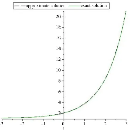
yields the exact solutions of the problem (see Figure 1). Example 3.2. We want to find the shortest distance from the point A(1,1,1) to the sphere
2 2 2 1
x y z
This problem is reduced to optimize the following functional:
, 1 1 2
2( )dJ
1
x
y z
y x z x x (19)point
where the B x y z
1, ,1 1
act solution y x,
must lie on the sphere,
with the ex 1 z1x
equations
, see [33]. The cor-
approximate solution exact solution
–3 –2 –1 0 1 2 3
t
20
18
16
14
12
10
8
6
4
[image:4.595.65.287.85.307.2]2
Figure 1. The graphs of approximated and exact solution for Example 3.1.
are:
2 2
dx 1y x z x
2 2
d
0,
d 0.
d 1
y
z
x y x z x
So that
2 2 , 2 2 .
1 1
y z
e f
y x z x y x z x
In above equations “e” and “f” are constant, so they
can be rewritten as:
2 2 2 2
1 0
1 0
y e y x x
f y x z
z
z x
,
.
The transversality conditions are:
1
2 2
2
2 2
1
1
0
x x
y y
y
x z
z
z
(20)
2 2 2 2
1 x y 1 y
z
z
1
2 2 2
2 2 . 0
1 1 1
x x
z
z z
y y
y y x y
2
2
1 1
0
1 n n d
n x
n n
y x y x
y s e y s z s sand
2
2
1 2
0
1 n n d
x
n n n
z x z x
z s f y s z s sThe variation from both sides of above equations for finding the optimal value of is:
1 1
0
n n n
1
1
0 d
d 0
x
x
n n s x n
y x y x y s s
y x y s y s s
and
1 2
0
d n x
n n
s x
z x z x z s s
2
2
0
d 0
x
n n n
z x z s z s s
Therefore
1 1
1 0,
s x s x
s s
0
.
and
2 2
1 0,
s x s x
s s
0
which yields:
1 s 1, 2 s 1.
So that the following iterative formulas are obtained:
1
2 2 0
1 ( ) 1 n n( ) d
n n
x n
y x y x
y s e y s z s s
1
2 2 0
( 1) 1 n n
n n
x n
z x z x
z s f y s z s s
If
d
0 , 0
y x ax b z x cxd then we have:
2 2
1 1 d
x
y ax b
a e a c s 02 2 1
e a c x b
and
2 2
1
0
2 2
1 d
1 x
z cx d c f a c s
f a c x d
2 (21)
1 1 , 1 1
.y b x b z d xd
1 3 0,
Imposing (20) and (21) lead to, 0, .
3
b d x
therefore:
which is the exact solution.
3.2. Isoperimetric Problems
Assume that two functions 1 , 1 . y x z x
, ,
G x y y and F x y y
, ,
are given. Among all curves
1
C x x0, 1 along yy x
which the functional
1
, ,
d x0
x
K y
G x y y xassumes a given value l, determine the one for which the
functional
0x
1
, , d
x
J y
F x y y xose that F and G have
partial derivatives for Gives an extermal value. Supp
continuous first and second
0 1
x x x and for arbitrary les y
and y.
Euler’s theorem: I
values of the variab
f a curve yy x
d
y x
extremizes the
functional J
1
0
, , x
x
y
F x y unde tr he conditions
1
0
, , d ,
x x
K y
G x y y xl
0 0,
1 1y x y y x y
and if yy x
is not an extremal of the functional K,there exists a constant such that the curve yy x
is an e al of the functional
sary condition for th
lem is to satisfy the Euler-Lagrange equation xtrem
1
, , d
x
L
F x y y xThe neces e solution of this
prob-
0
, , x
G x y y
d 0
d
H H
y x y
with given boundary conditions in which H F G
for further information (see [2]). ple 3.3.
Exam It is aimed to find the minimum of the
functional
π
2
0 d
J y
y x x (22)Such that
and
π
2
0
d 1
y x x
(23)
0 0,
π 0y y (24)
With exact solution y x
2sinx [19].Accord-
xan sponding Euler-Lagrange equation:
π
ing to the following auxiliary functional:
1
2 2
0
d
L
y yd the corre
y 0 d2 2
d
y x
so
0
y y
By applying He’s variational iterative method results
To find the optimal value of
0
d
y 1 x y
y s xn n x
yn s following equation is required:
1
n n n s x
x
y x y x y s
0
[ yn s ]s x yn s yn s ds
0
herefore, the stationary conditions are obtained in the following form:
T
( ) 0,
0. s x
s x
s
1s x 0,
which yields
s x
and the desired sequence is
1
0
d
x
n n n n
y x y x
sx y s y s sBy choosing y0 a sin
cx bcos
cx
1
2 2
0
2 2 2
cos
( ) sin cos d
sin cos
x
x b cx
sin
y x a c
s x ac a cs b b cs s
a cx b cx b ax
b acx
c
c c
Imposing (24) on this function given
c
c
1 2
si
a
n
0, cx ax
b y x acx
c c
0
If then from (24) ac0, but from (23)
3 3 ,
π
ac which is a contra
Now imposing (24), we have: diction.
3π
sin π π
c
c c
so 0. and it is known that in this case imposing (24) on the Euler Lagrange equation yields
2
, 1,
c k k 2,
Hence:
siny x a kx
and from (23) 2
π
a . But y must be extremal when
, therefore:
0 x π
2sinπ
y x x
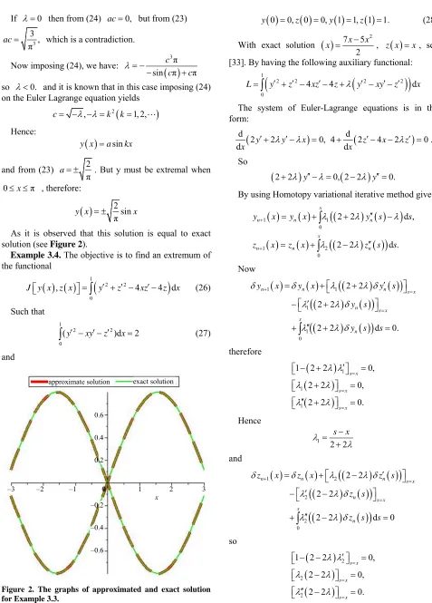
lution is equal to e ct
4 d
As it is observed that this so xa
solution (see Figure 2).
Example 3.4. The objective is to find an extremum of the functional
1
2 2
0
, 4
x z x y z xz z
J y
x (26)Such that
and
2
0
)d 2
z x
(27) 1
2 (y xy
approximate solution exact solution
x
–3 –2 –1 0 1 2 3 0.6
0 0, 0
0, 1
1, 1
1y z y z . (28)
With exact solution
2
7 5
2
x x
x , z x
x, see[33]. By having the following auxiliary functional:
The system of Euler-Lagrange equations is in the form:
1
2 2
0
2 4 4 2 d
L
y z xz z y xy z x
d d
2 2 0, 4 2 4 2
dx y yx dx z x z 0.
So
2 2
y 0, 2 2
y0.By using Homotopy variational iterative method gives:
Now
1 1
1 2
0
2 2 d ,
2 2 d .
x
n n n
x
n n n
y x y x y s s
x z s s
0
z x z
1 1
1
1
2 2
2 2
2 2 d 0.
n n n
0
s x
y x y x y
n
s x x
n
s
y s
y s s
therefore
11 2 2 0,
s x
1
1
2 2 0,
2 2 0.
s x
s x
Hence
0.4
0.2
–0.2
–0.4
[image:6.595.55.532.71.736.2]–0.6
Figure 2. The graphs of approximated and exact solution for Example 3.3.
1 2 2
s x
and
1 2
2
2 0
2 2
2 2
2 2 d 0
n n s x
n s x
n n
x
z x z x z s
z s
z s s
so
2
2
2
1 2 2 0,
2 2 0,
2 2 0.
s x
s x
s x
So 2 is obtained as:
2
2 2
s x
and the following iterative equations are obtained:
1
0
2 2 d
2 2
x
n n n
s x
y x y x y s
s,
1
0
2 2 d .
2 2 x
n n n
s x
z x z x z s s
By choosing y0ax b z , 0cxd:
1
0 2
1
d 2 2
,
4(1 )
x
s x
y x ax b s
x ax b
z cx d
And by imposing (28) on this functions:
2
1
1
1 ,
4 1
a
0, 1, 0,
1 ,
4 1 4 1
b c d
x
y x x
from (27):
z x
1 2
10 12
,
11 11
And consequently:
approximate solution exact solution
x
–10
–20
–30
[image:7.595.57.298.118.708.2]–3 –2 –1 0 1 2 3
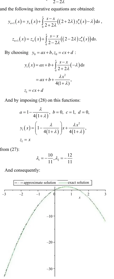
Figure 3. The graphs of approximated and exact solution for Example 3.4.
7 5 2,
2x x
y x z x x.
which is the exact solution (see Figure 3).
4. Conclusion
The He’s variational iterative method is an efficient me-thod for solving various kinds of problems. In this paper variational iterative method is employed for finding the minimum of a functional with moving boundaries and isoperimetric problems. Using He’s variational iterative method the solution of the problem is provided in a closed form. Since this method does not need to the dis-cretize of the variables, there is no computational round off error. Moreover, only a few numbers of iterations are needed to obtain a satisfactory result.
REFERENCES
[1] P. G. Engstrom and U. Brechtken-Manderschied, “Intro-ew York, 1991.
[2] A. Saadatmandi and M. Dehghan, “He’s Variational It-eration Method for Solving a Partial Differential Equation Arising in Modeling of Water Waves,” Zeitschrift für
7.
al Iteration Method a Kind of Non- al Technique: Some Examples,”
Interna-duction to the Calculus of Variations,” Chapman and Hall/CRC, N
Naturforschung, Vol. 64, 2009, pp. 783-78
[3] J. H. He, “Variation Linear Analytic
tional Journal of Nonlinear Mechanics, Vol. 34, No. 4,
1999, pp. 699-708. doi:10.1016/S0020-7462(98)00048-1
[4] M. A. Abdou and A. A. Soliman, “Varitional Iteration Method for Solving Burgers’ and Coupled Burgers’ Equ-ations,” Journal of Computational and Applied Math- matics, Vol. 181, 2005, pp. 45-251.
[5] J. Biazar and H. Ghazvini, “He’s Variational Iteration Method for Solving Hyperbolic Differential Equations,”
International Journal of Nonlinear Sciences and Nu-merical Simulation, Vol. 8, 2007, pp. 311-314.
[6] M. Dehghan and M. Tatari, “The Us
Iteration Method for Solving a Fokker Plancke of He’s Variational Equation,”
Physica Scripta . 310-316. doi:10.1088/00
, Vol. 74, No. 3, 2006, pp
31-8949/74/3/003
[7] M. Dehghan and A. Saadatmandi, “Variational Iteration Method for Solving the Wave Equation Subject to an In-tegral Conservation Condition,” Chaos, Solitons and Fr- actals, Vol. 41, No. 3, 2009, pp. 448-1453.
doi:10.1016/j.chaos.2008.06.009
[8] M. Dehghan and F. Shakeri, “Approximate Solution of a Differential Equation Arising in Astrophysics Using the Variational Iteration Method,” New Astronomy, Vol. 13,
No. 1, 2008, pp. 53-59. doi:10.1016/j.newast.2007.06.012
e of Variational I [10] M. Dehghan and R. Salehi, “The Us
tera-tion Method and Adomian Decompositera-tion Method to Solve the Eikonal Equation and Its Application in the Reconstruction Problem,” Communications in Numerical Methods in Engineering, in press.
[11] M. Dehghan and M. Tatari, “The Use of Adomian De-composition Method for Solving Problems in Calculus of Variations,” Mathematical Problems in Engineering, Vol.
2006, 2006, pp. 1-12. doi:10.1155/MPE/2006/65379
[12] M. Dehghan and M. Tatari, “Identifying an Unknown Function in a Parabolic Equation with over Specified Da-ta via He’s Variational Iteration Method,” Chaos, Solitons and Fractals, Vol. 36, 2008, pp. 57-166.
[13]J. H. He, “Variational Iteration Method for Autonomous Ordinary Differential Systems,” Applied Mathematics and Computation, Vol. 114, No. 2-3, 2000, pp. 115-123. doi:10.1016/S0096-3003(99)00104-6
[14] J. H. He and X. H. Wu, “Variational Iteration Method: New Development and Applications,” Computers and Mathematics with Applications, Vol. 54, No. 7-8, 2007, pp. 881-894. doi:10.1016/j.camwa.2006.12.083
[15] J. H. He, “Variational Iteration Method: Some Recent Results and New Interpretations,” Journal of Computa-tional and Applied Mathematics, Vol. 207, No. 1, 2007,
pp. 3-17. doi:10.1016/j.cam.2006.07.009
[16] J. H. He, Variational Iteration Method for Delay Differ-ential Equations,” Communications in Nonlinear Science and Numerical Simulation, Vol. 2, No. 4, 1997, pp. 235-
236. doi:10.1016/S1007-5704(97)90008-3
[17] J. H. He, “Approximate Solution of Nonlinear Differen-tial Equations with Convolution Product Nonlinearities,”
Computer Methods in Applied Mechanics and Engineer-ing, Vol. 167, No. 1-2, 1998, pp. 69-73.
doi:10.1016/S0045-7825(98)00109-1
[18] J. H. He, “Approximate Analytical Solution for Seepage Flow with Fractional Derivatives in Porous Media,”
Computer Methods in Applied Mechanics and Engineer-ing, Vol. 167, No. 1-2, 1998, pp. 57-68.
doi:10.1016/S0045-7825(98)00108-X
[19] M. Inc, “Numerical Simulation of KdV and mKdV Equa-tions with Initial CondiEqua-tions by the variational Iteration Method,” Chaos, Solitons and Fractals, Vol. 34, No. 4, 2007, pp. 1075-1081. doi:10.1016/j.chaos.2006.04.069
[20] S. Momani and S. Abuasad, “Application of He’s Varia-tional Iteration Method to Helmholtz Equation,” Chaos, Solitons and Fractals, Vol. 27, No. 5, 2006, pp. 1119- 1123. doi:10.1016/j.chaos.2005.04.113
[21] S. Momani and Z. Odibat, “Analytical Approach to Lin-ear Fractional Partial Differential Equations Arising in Fluid Mechanics,” Physics Letters A, Vol. 355, No. 4-5,
2006, pp. 271-279.
doi:10.1016/j.physleta.2006.02.048
[22] H. Ozer, “Application of the Variational Iteration Method to the Boundary Value Problems with Jump Discontinui-ties Arising in Solid Mechanics,” Interna
Nonlinear Sciences and Numerical S
tional Journal of imulation, Vol. 8,
ar
2007, pp. 513-518.
[23] Z. M. Odibat and S. Momani, “Application of Variational Iteration Method to Nonlinear Differential Equations of Fractional Order,” International Journal of Nonline Sciences and Numerical Simulation, Vol. 7, 2007, pp. 27- 34. doi:10.1515/IJNSNS.2006.7.1.27
[24] H. Sagan, “Introduction to the Calculus of Variations,” Courier Dover Publications, 1992.
[25] F. Shakeri and M. Dehghan, “Numerical Solution of the Klein-Gordon Equation via He’s Variational Iteration Method,” Nonlinear Dynamics, Vol. 51, No. 1-2, 2008, pp. 89-97. doi:10.1007/s11071-006-9194-x
[26] tion of a Model
De-scribing Biological Species Living Together Using the Variational Iteration Method,” Mathematical and Com-puter Modeling, Vol. 48, No. 5-6, 2008, pp. 685-699. F. Shakeri and M. Dehghan, “Solu
doi:10.1016/j.mcm.2007.11.012
M. Tatari and M.
[27] Dehghan, “Solution of Problems in Calculus of Variations via He’s Variational Iteration Me-thod,” Physics Letters A, Vol. 362, No. 5-6, 2007, pp.
401-406. doi:10.1016/j.physleta.2006.09.101
[28] M. Tatari and M. Dehghan, “Improvement of He’s Varia-tional Iteration Method for Solving Systems of
Differen-p. 2160-2166. tial Equations,” Computers and Mathematics with Appli-cations, Vol. 58, No. 11-12, 2009, p
doi:10.1016/j.camwa.2009.03.081
[29] M. Tatari and M. Dehghan, “On the Convergence of He's Variational Iteration Method,” Journal of Computational and Applied Mathematics, Vol. 207, No. 1, 2007, pp. 121- 128. doi:10.1016/j.cam.2006.07.017
[30] S. A. Youse and M. Dehghan, “The Use of He’s Varia-tional Iteration Method for Solving VariaVaria-tional Prob-lems,” International Journal of Computer Mathemat
Vol. 87, No. 6, 2010.
ics, /00207160802283047 doi:10.1080
[31] A. M. Wazwaz, “A Comparison between the Variational Iteration Method and Adomian Decomposition Method,”
Journal of Computational and Applied Mathematics, Vol. 207, No. 1, 2007, pp. 129-136.
doi:10.1016/j.cam.2006.07.018c
[32] R. Memarbashi, “Variational Problems with Moving Boun- daries Using Decomposition Method,” Mathematical Problems in Engineering, Vol. 2007, 2007, Arti
10120. cle ID