A New Type of Phase Transition Based on the Clausius Clapeyron Relation Involving a Change in Spatial Dimension

(1)

http://www.scirp.org/journal/jhepgc ISSN Online: 2380-4335

ISSN Print: 2380-4327

DOI: 10.4236/jhepgc.2019.52016 Feb. 15, 2019 291 Journal of High Energy Physics, Gravitation and Cosmology

A New Type of Phase Transition Based on the

Clausius-Clapeyron Relation Involving a Change

in Spatial Dimension

Christopher Pilot

Physics Department, Gonzaga University, Spokane, WA, USA

Abstract

Using a space filled with black-body radiation, we derive a generalization for the Clausius-Clapeyron relation to account for a phase transition, which in-volves a change in spatial dimension. We consider phase transitions from dimension of space, n, to dimension of space,

(

n−1

)

, and vice versa, from

(

n−1

)

to n-dimensional space. For the former we can calculate a specific

release of latent heat, a decrease in entropy, and a change in volume. For the latter, we derive an expression for the absorption of heat, the increase in en-tropy, and the difference in volume. Total energy is conserved in this trans-formation process. We apply this model to black-body radiation in the early universe and find that for a transition from n=4 to

(

n− =1

)

3, there is an

immense decrease in entropy accompanied by a tremendous change in volume, much like condensation. However, unlike condensation, the volume change is not three-dimensional. The volume changes from V4, a four-dimensional con-struct, to V3, a three-dimensional entity, which can be considered a subspace of V4. As a specific example of how the equation works, we consider a transi-tion temperature of 3 × 1027_{Kelvin, and assume, furthermore, that the latent} heat release in three-dimensional space is 1.8 × 1094_{Joules. We find that for this} transition, the internal energy densities, the entropy densities, and the volumes assume the following values (photons only). In four-dimensional space, we

ob-tain, 125 4

4 1.15 10 J m

u = × ⋅ − , 97 4 1

4 4.81 10 J m K

s = × ⋅ − ⋅ − , and

31 4

4 2.14 10 m

V = × − . In three-dimensional space, we have

94 3

3 6.13 10 J m

u = × ⋅ − , 67 3 1

3 2.72 10 J m K

s = × ⋅ − ⋅ − , and 3

3 0.267 m

V = . The

subscripts 3 and 4 refer to three-dimensional and four-dimensional quanti-ties, respectively. We speculate, based on the tremendous change in volume, the explosive release of latent heat, and the magnitudes of the other quantities calculated, that this type of transition might have a connection to inflation. How to cite this paper: Pilot, C. (2019) A

New Type of Phase Transition Based on the Clausius-Clapeyron Relation Involving a Change in Spatial Dimension. Journal of High Energy Physics, Gravitation and Cosmology, 5, 291-309.

https://doi.org/10.4236/jhepgc.2019.52016

Received: January 8, 2019 Accepted: February 12, 2019 Published: February 15, 2019

(2)

DOI: 10.4236/jhepgc.2019.52016 292 Journal of High Energy Physics, Gravitation and Cosmology

With this work, we prove that space, in and of itself, has an inherent energy content. This is so because giving up space releases latent heat, and buying space costs latent heat, which we can quantify. This is in addition to the energy contained within that space due to radiation. We can determine the specific amount of heat exchanged in transitioning between different spatial dimensions with our generalized Clausius-Clapeyron equation.

Keywords

Clausius-Clapeyron Relation, Spatial Dimension, Phase Transition, Inflation

1. Introduction

As is well known, the Clausius-Clapeyron relation [1] [2] [3] [4] is useful in pre-dicting the latent heat given off when a substance undergoes a first order phase transition at a particular temperature and pressure. A first order phase transition is a discontinuous phase transition for which there is an abrupt change in phase, and latent heat is released or absorbed by a fixed amount. The discontinuity is characterized by a co-existence curve, typically plotted as pressure versus tem-perature, and on this curve, both phases can co-exist at specific temperatures and pressures. We assume a closed system where temperature and pressure are clearly defined on either side of this curve, and are held constant at a particular point on the curve when transitioning.

The Clausius-Clapeyron relation, as presently formulated, assumes that space is smooth, continuous, and three-dimensional, both before and after a transition. We relax the assumption of dimensionality. We will show that it is possible to generalize this important thermodynamic relation to include phase transitions, which are changing spatial dimension itself, while all the while conserving total energy. Furthermore, this kind of analysis may prove consequential in under-standing the inflation phase of the early universe.

Our motivation for studying this problem is three-fold. First, it is of general theoretical interest for compactification and Kaluza-Klein theories [5]-[10]. When symmetries are broken, whether spontaneously or otherwise, the dimen-sionality of space often remains fixed, but not in compactification. What does it mean if spontaneous symmetry breaking occurs thermodynamically with an attendant change in spatial dimension? While we will not attempt to address this question in detail, we will show how it can be done. The key is the Clau-sius-Clapeyron equation.

(3)

spa-DOI: 10.4236/jhepgc.2019.52016 293 Journal of High Energy Physics, Gravitation and Cosmology

tially changing phase transition from n = 4 dimensions to n = 3 dimensions, may offer the order of magnitude scales required for early cosmic evolution, and for inflation in particular. In addition, because it happened at an instant, then and there so to speak, with a tremendous release of latent heat, thermal equilibrium was guaranteed shortly thereafter. Moreover, the problem with a-causal expo-nential expansion may not be an issue if it is the space itself, which is expanding upon changing dimensions when transitioning. Finally, in regards to inflation, we will also show that relative fluctuations in temperature, δT T, can be carried

over, or even created in certain circumstances, when transitioning from one space to another neighboring space. This appears to be a unique feature for this kind of transformation as will be demonstrated.

Third, we recently presented a paper [11] where we advanced the notion that the universe may be modeled as a thermodynamic heat engine. There, we as-sumed a closed universe, i.e. one with a slight positive curvature, which will al-low for a big bounce scenario. To explain inflation, and expansion in general, we proposed a Carnot cycle for the cosmos consisting of isothermal expansion (from points,

a

→

b

), adiabatic expansion (from points,

b

→

c

), isothermal

contraction (form points,

c

→

d

) and isothermal contraction (from points,

d

→

a

). The universe finds itself currently in the adiabatic expansion mode.

This four step process brings the universe back to its initial configuration, point a, where we have a finite temperature, a finite pressure, a finite energy, a finite volume, etc. The universe, being cyclic, has no real beginning, nor does it have an end. Spatially, there are no “edges” as the universe has no boundaries. The in-flation phase is identified as the initial isothermal expansion phase, from points,

a

→

b

. This very short phase did not last long, of the order of only, 10−35 s.

Time evolved very differently in the isothermal expansion mode, as was shown explicitly in reference [11]. Time evolution was not temperature depen-dent, but, interestingly, volume dependent. The volume expanded by a factor of only 5.65, as did total entropy, and this expansion was fueled by thermal quan-tum fluctuations and heat transfer from surroundings to system. We identified the “surroundings” as those parts of the observable universe, which spatially in the WMAP and Planck maps are now slightly cooler. Those are the pockets of space where matter later aggregated. The “system” consisted of voids, i.e. those parts of space that do the actual expanding currently. These regions were slightly hotter in the very early universe. The adiabatic expansion phase, which follows isothermal expansion, is driven by a different mechanism, a decrease in internal energy. The specifics are given in reference [11].

The connection between this model and a spatially changing phase transition from n=4 to

(

n− =1

)

3 space dimensions is as follows. This phase transition

(4)

than likely, on the low side1_{[12] [13] [14]}_{. We also made use of the present} ra-dius of the observable universe, about 4.4 × 1026_{m, which is in itself, a very} crude approximation. The temperature for the isothermal process was ascer-tained to be about 3 × 1027_{K. This number was derived using Heisenberg’s} un-certainty principle, and the slight spatial temperature variations found in the WMAP and Planck missions, namely, 5

5 10

T T

δ _{≈ ± ×} − _{between the hot and}

cold spots found within the photon blackbody radiation. Perhaps the source for the heat required for the isothermal phase was not the transfer of heat from sur-roundings to system as originally proposed in reference [11]. Perhaps it is due to a spatially changing phase transition from n = 4 to

(

n− =1

)

3 at _T _{≈ ×}_{3 10}27 _K.

Irrespective of whether our heat engine model is valid, we consider the generali-zation of the Clausius-Clapeyron relation to be of paramount importance for both thermodynamics, and an understanding of compactification theory in gen-eral.

Recently, researchers [15] have suggested that a n=4 to

(

n− =1

)

3

transi-tion might actually have occurred in the very early universe. At a temperature of 0.93 × Planck Temperature they found that the Helmholtz free energy density function reaches a maximum value when plotted as a function of spatial dimen-sion,

n

=

1, 2,3, 4,



. That maximum was reached for n≈3. This was the first

of several important thermodynamic variables to do so, and they interpreted this extremum as the transition point where nature decided on three spatial dimen-sions. While we agree with their overall premise that compactification may have occurred, we disagree with their estimate for the temperature of this transition. The Planck temperature is 1.42 × 1032_{K, and 93% of this is still +10}32_{K. We} be-lieve in a lower temperature for the n=4 to

(

n− =1

)

3 transition, which we

call T43=T34. We believe it is closer to 3 × 10

27_{K based on our heat engine}

1_{At a temperature of} 27

3 10 K∗ , it is well known that there are many species of radiation present, not just photons. There are the neutrinos

(

ν ν ν ν ν νe e, µ µ, τ τ

)

, and the e e,µ µ τ τ,

+ − + − + −_{pairs which contribute to}

radiation. We also have quark, antiquark and gluon radiations. Then there are 0

, ,

W W+ − Z radiative contributions, etc. If we take just the particles in the standard model into consideration, then we have as the energy density ( )

(

2

)

*( ) 4

30

u T = π g T T where *( ) ( ) ( )

7 8

b f

g T =g T + g T , and gb=

∑

gi is the sum over relativistic bosonic species. The gf =

∑

gi is the corresponding sum over relativistic fermions. The *( )

g T counts up the effective number of relativistic degrees of freedom (photons count as two degrees of freedom), which is temperature dependent for massive particles. All particles in the standard model are already relativistic at temperatures of 16

10 K≈1TeV. When we carry out the sum for the known particle species, we obtain gb=28, gf=90, and, therefore,

*

106.75

g = . We would also have to add those particles which are not yet observed, but which could exist in the form of radiation at 27

3 10 K∗ such as supersymmetric particles, dark matter particles, etc. To make a long story short, the input heat needed to bring these types of radiations into thermal equili-brium with the photons is therefore higher, than if we just consider photons by themselves. There-fore, our original rough estimate of 94

1.8 10 J

L= ∗ is, most probably, too low in value and we should multiply this number by a scale factor such as *( )

(5)

model, as well as other considerations. Regardless of what the actual transition temperature turns out to be, assuming it exists, we approach the problem of a spatial phase transition from an entirely different perspective. We focus on the Clausius-Clapeyron (abbreviated CC) relation and generalize the relation to ap-ply for a spatial change in phase; in other words, the dimension of space changes.

The outline of this paper is as follows. In Section II, we generalize the CC rela-tion using radiarela-tion as the substance filling space. We believe that radiarela-tion in all its forms (photons, neutrinos, e+_e−_{pairs, etc.) is the primordial substance found} in the very early universe when temperatures were very high. Radiation will de-fine space according to Mach’s principle (matter/energy content dede-fines space) and spatial transitions are assumed possible. To keep the discussion simple we will focus exclusively on photons. In very general terms we derive the generaliza-tion of the CC equageneraliza-tion for an arbitrary n-dimensional to

(

n−1

)

-dimensional

spatial change of phase, and vice versa. We also consider the conservation of energy and changes in hypervolume in general terms. In Section III we focus on the transition from n=4 to

(

n− =1

)

3. We will assume specific values for

temperature of transition, as well as amount of latent heat release, in order to show how the equation works. The specific values chosen are motivated by pre-vious work [11]. Quantities in three-dimensional and four-dimensional spaces are then calculated, such as entropy and volume, both before and after. In Sec-tion IV, we discuss inflaSec-tion in general, and consider our n= →4

(

n− =1

)

3

model in particular. The WMAP and Planck satellite missions show a remarka-ble uniformity in photon blackbody temperature. Nevertheless, there is a slight inhomogeneity in temperature, which explains the present structure of the un-iverse. That inhomogeneity is of the order, 5

5 10

T T

δ _{= ± ×} − _._{How does this}

non-uniformity in temperature behave when undergoing a spatially changing phase transition? How, specifically, are the other thermodynamic quantities af-fected? We will answer both questions in Section IV. Finally, in Section V, we present our summary and conclusions.

2. Generalization of the Clausius-Clapeyron Relation

In this section, we generalize the CC relation to allow for a phase transition from

n-dimensional space to

(

n−1

)

-dimensional space and vice versa. We start with

the internal internal radiation energy density (photons only). As is known [16] [17] [18] [19], the internal energy density in n-dimensional space is given by the following function, which depends only on temperature and the dimensionality of space, n:

(

) (

)

2

(

)

1

(

) (

) ( ) ( )

, 2 1 πn B n 1 1 n 2

u=u n T = n− k T +

ζ

n+ Γ +n _ hc Γ n _ (2-1)

In this equation, kB is Boltzmann’s constant, c equals the speed of light, h is

Planck’s constant, ζ

( )

x is the zeta function, and Γ

( )

x is the gamma func-tion. From this function, we can furthermore show that

(

)

, , 1

(6)

Here, “f” is the Helmholtz free energy density, “p” is the pressure, and “s” is the entropy density. The Helmholtz function is defined as F≡U–TS, and therefore, f = −u Ts.

In n-dimensional space, a hypervolume can be defined for a n-dimensional ball. The expression [20] [21] is

( )

π

2

( )

₁

2

n n

n n n n

n

V

=

V R

=

R

Γ



_

+



_





(2-3) The subscript “n” on a physical quantity will always refer to the spatial dimen-sion in which the quantity is defined. Γ

( )

x is again the gamma function.

If we specialize to three spatial dimensions, n=3, then we obtain familiar

formulas using the equations above:

(

) ( )

4 3

5 3

3 8 15π B , 3 3 3, 3 4 3 3 , 3 4 3π 3

u = k T hc p =u s = u T V = R (2-4)

The internal energy density is often written as 4 4 3 4

u = σT c=AT , where σ is the Stefan-Boltzmann constant, and A has the numerical value equal to

16 3 4

7.566 10× − J m⋅ − ⋅K− . For = 4, V₄ equals

( )

π 2

2

( )

R

4 4, and in two dimen-sions,

( )

2

2 π 2

V = R . When not specified explicitly, we use MKS units throughout this paper.

Next, we consider the entropy in n-dimensional space. We find that

(

1

) (

)

n n n n n

S =s V = n+ n u T V (2-5) For

(

n−1

)

-dimensional space, we obtain

(

)(

)

1 1 1 1 1 1

n n n n n

S ₋ =s V₋ ₋ =n n− u ₋ T V₋ (2-6)

We can also calculate, using Equation (2-2) and Equation (2-1),

(

dp_n dT V

)

_n. The result is

(

dp_n dT V

)

_n =

(

n+1

) (

n u T V_n

)

_n (2-7)

Similarly,

(

dpn−1 dT V

)

n−1 =n n

(

−1

)(

un−1 T V

)

n−1 (2-8)

Comparing right hand sides of Equation (2-5) and Equation (2-7), it is clear that

(

d d

)

n n n

S = p T V (2-9) Similarly, comparing right hand sides of (2-6) and (2-8), we see that

(

)

1 d 1 d 1

n n n

S₋ = p₋ T V₋ (2-10) Therefore, if we take the difference between Equation (2-9) and Equation (2-10), we find that

(

)

(

)

1 d d d 1 d 1

n n n n n n

S −S ₋ = p T V − p ₋ T V₋ (2-11) This is our generalization of the CC relation. The difference in entropy mul-tiplied by the temperature is the latent heat,

∆

Q

. Therefore, Equation (2-11)

(7)

(

)

(

)

1 d d d 1 d 1 1 2

n n n n n n

S −S ₋ = p T V − p₋ T V₋ = ∆Q T (2-12) The factor of 1/2 on the right hand side of Equation (2-12) will be explained shortly. Equation (2-12) is dimensionally consistent, as we shall also soon see, even though the densities and pressure are defined in different dimensions, and thus have different units.

The general expression for ∆ =S

(

Sf –Si

)

is d

f

i

S Q T

∆ =

_∫

_{. The}S_n and

1

n

S − in Equation (2-12) can be thought of as entropy states, Si and Sf .

However, if the temperature is held fixed, as in a first order phase transition, this reduces to ∆ = ∆S Q T. When written out,

(

S_f –S_i

) (

= Q_f –Q_i

)

T. The sign of ∆S determines the sign of

∆

Q

. It will soon become apparent that S_n =S_i

is always greater than Sn−1=Sf . Therefore,

∆

Q

in (2-12) is positive which

means that heat is being given off in the final state. If we reverse the transition from

(

n−1

)

-space to n-space, we simply multiply Equation (2-12) by a minus

sign. In this instance, Sn =Sf and Sn−1=Si and

∆

Q

is negative. This means

that latent heat has to be supplied for this transition to occur. The

∆

Q

is often

written as L, which stands for latent heat. Barring exotic scenarios where we have parallel universes or multi-universes, etc., we will assume that the latent heat, which is released in the first type of transition where we decrease the num-ber of dimensions, will be released in

(

n−1

)

-space. For the second type of

transition, where we increase the dimensionality of space, the heat which needs to be supplied in order for this transition to happen, needs to come from the originating

(

n−1

)

-space.

Equation (2-12) reduces to the conventional CC relation (up to a factor of 1/2) in the limit where n equals

(

n−1

)

, if we can imagine such a limit allowing for

1

n n

S ≠S − and Vn≠Vn−1. Both temperature and dimension of space are similar in this limit, and thus, there is no difference between pn and pn−1. We retrieve the standard CC equation in Equation (2-12), except for the factor of 1/2. Therefore, in an intriguing way, the familiar CC relation is obtained as a special case when neighboring spaces converge. Since a first order phase transition is a discontinuous phase transition, we can easily imagine that Sn ≠Sn−1 and

1

n n

V ≠V₋ , even though the dimensions of space are now the same in this special

limit.

Let us next prove that Equation (2-12) is dimensionally consistent. We note that, in terms of units, the dim T

[ ]

n =dim T

[ ]

n−1 =dim T

[ ]

. However, Equation

(2-1) shows us that

[ ]

( 1)

1

J m n J m n

n n

dim u = ⋅ − ≠dim u₋ = ⋅ − − (2-13) We are working within the MKS system where “J” stands for Joules and “m” for meters. From relations (2-13) and (2-2b), we also notice that

[ ]

( )

_[

_]

( ) ( )

1 2

1 1

N m n N m n

n n n n

dim p =dim u = ⋅ − − ≠dim p₋ =dim u_ ₋ _= ⋅ − − (2-14)

Here “N” refers to 1

(8)

[ ]

1

[ ]

( 1) 1

1

J m n K J m n K

n n

dim s = ⋅ − ⋅ − ≠dim s− = ⋅ − − ⋅ − (2-15)

The “K” refers to degrees Kelvin. Moreover, from Equation (2-3) we see that

[ ]

( 1) ( 1)

n n

dim V =m ≠dim V_ ₋ _=m − (2-16)

From these relations, it is easy to prove that

[ ]

n

[ ]

n

[ ]

n J

[

n 1

]

[ ]

n1

[ ]

n1

dim U =dim u ∗dim V = =dim U ₋ =dim u ₋ ∗dim V₋ (2-17)

[ ]

n

[ ]

n

[ ]

n J K

[

n1

]

[ ]

n1

[ ]

n1

dim S =dim s ∗dim V = =dim S ₋ =dim s₋ ∗dim V₋ (2-18) The quantities, Un and Sn, refer to the internal energy and entropy in

n-spatial dimensions, and we notice that these quantities do not depend on the value of “n” as far as dimensional units are concerned. We can substitute the dimensionalities specified above into Equation (2-12) to show that the Equation (2-12) is, indeed, dimensionally correct.

We now explain the factor of 1/2 in Equation (2-12). Conservation of energy, in all its forms, between spatial dimensions demands that

1 1 1 1

n n n n n n n n

U +p V +S T =U − +p V− − +S−T+L (2-19)

In this equation, L is the latent heat released in

(

n−1

)

-dimensional space,

which may or may not equal zero, at this stage (It will turn out that L is unequal to zero and positive later). The various terms on the left hand side of (2-19) represent the internal energy, the stored work, and the heat content of photons, respectively, in 𝑛𝑛-dimensional space. We have the same on the right hand side but in

(

n−1

)

-dimensional space, plus any latent heat, which may, or may not,

be released in

(

n−1

)

space. We can simplify Equation (2-19), utilizing

Equa-tion (2-2b). Upon substituEqua-tion of the latter expression, we now write (2-19) as

(

n+1

)

n Un+S Tn = n n

(

−1

)

Un−1+Sn−1T+L

   

    (2-20)

We can simplify (2-19) further using (2-2c) to eliminate Sn and Sn−1. Here we obtain

(

)

(

)

1

2_ n+1 n U_ _n =2_n n−1_U_n₋ +L (2-21)

Alternatively, we use Equation (2-2c) to eliminate Un and Un−1 in Equa-tion (2-20) and find that

1

2S Tn =2Sn−T+L (2-22)

However, from the paragraph following Equation (2-12), we saw that

(

)

(

)

1 1

– – – –

f i n n f i n n

S S =S ₋ S = Q Q T = Q₋ Q T = −L T (2-23)

(9)

sides. As it turns out, the sum of internal energy and stored work is numerically equal, in each dimension, to the stored heat in that dimension. Therefore, we have the extra factor of two in both Equation (2-21) and Equation (2-22). Whe-rever we see Q or L in Equation (2-23), we should substitute 1/2Q, and 1/2L. Another way of saying the same thing is that twice the entropy change is needed to release a fixed amount of latent heat, L, due to the requirement of maintaining internal energy and stored work, in both spaces. See Equation (2-22). Equation (2-22) is another way to write our generalized CC equation, Equation (2-12). One cannot just transfer internal energy for photons, and leave the associated pressure and entropy behind. It’s all or nothing if a transition occurs.

We close this section by deriving an expression for the hypervolume ratio,

(

V Vn n−1

)

, as this will be needed later on. We start with Equation (2-21), which

we rewrite as

(

)

(

)

1 1 1

2_ n+1 n u V_ _n _n =2_n n−1 _u V_n₋ _n₋ +L_n₋ (2-24) On the right hand side of (2-24), we have made explicit the fact that L is de-fined in

(

n−1

)

-space. We next define latent heat density as l_n≡L V_n _n. This

allows us to reformulate Equation (2-24) as follows:

(

)

(

)

2 2

1 – 1 1 2 1 1

n n n n n n

V V− =n n u − u +n n+ l− u (2-25)

Therefore,

(

)

(

)

2 2

1 1 – 1 2 1 1 1

n n n n n n

V V₋ =u₋ u _n n +n n+ l₋ u₋ _ (2-26)

or, alternatively,

(

)

(

)

2 2

1 1 – 1 2 1 1 1

n n n n n n

V V− =u− u _n n +n n+ L− U − _ (2-27)

The latent heat is released in

(

n−1

)

space for a transition from spatial

di-mension, n, to spatial dimension,

(

n−1

)

. As mentioned previously, we will not

consider exotic situations where the heat can be released in any other kind of space, such as in a parallel universe, multi-universes, etc.

Both Equation (2-26) and Equation (2-27), are linear equations where the de-pendent variable can be considered

(

V Vn n−1

)

and the independent variable is

either ln−1 for Equation (2-26), or Ln−1 for Equation (2-27). We will be look-ing at a transition from n=4 to

(

n− =1

)

3 in the next section, and it is more

likely that we can give an estimation of either ln−1 or Ln−1, versus

(

V Vn n−1

)

.

(10)

e+_e−_{radiation annihilation and heating up of photons. For}_T_{we substitute} 43

T ,

the transition temperature, and for T0, we insert the present temperature of the photon blackbody radiation, which is T0=2.7255 K. Therefore, we estimate

that 3

(

)

3 3

(

)

(

26

)

3

3 present observable volume 0 4π 3 4.4 10 m

V =a × =a V =a × . For

a specific transition temperature of 3 × 1027_{K, we obtain} 3

3 0.267 m

V = .

We can easily read off the slope and y-intercept, in both Equation (2-26) and Equation (2-27). Both slope and y intercept are transition temperature depen-dent, and only transition temperature dependent for a given “n” to

(

n−1

)

transition. For any latent heat release in

(

n−1

)

space, we can calculate the

vo-lume in n-space using either Equation (2-26) or Equation (2-27).

3. The n = 4, to (n

−

1) = 3, Transition

In this section, we consider the n=4 to

(

n− =1

)

3 transition. We start with

the generalized CC equation, Equation (2-12). We specialize to n=4, and

ob-tain

(

S4−S3

) (

= dp4 dT V

)

4−

(

dp3 dT V

)

3 =1 2∆Q T (3-1)

Written more elegantly, we use Equation (2-22), which is the equivalent. We focus on this second version, and write

(

S4−S3

)

=1 2L T (3-2)

Our task is to find the hypervolume, V4, using this equation, as well as other thermodynamic quantities of interest in 3-space and 4-space for a specific tran-sition temperature. We start with Equation (2-1), where we first evaluate u3 and u4. We will assume a transition temperature of 3 × 10

27_{K. Upon evaluating} the constants and inserting this temperature, we find:

( ) ( ) (

) ( )

(

) ( )

4 16 4 94 3

3

4 3 3

125 4 3

7.566 10 6.128 10 J m and

5 4 3 2 1.437

627.6 1.154 10 J m

B B

u AT T

u u k T ћc u k T ћc

u T

ζ ζ

−

= = × × = ×

= × × × = × ×

= × × = ×

(3-3)

MKS units will be used exclusively in this paper (even though, sometimes, we will not always write them out). We next evaluate the radiation pressure in both spaces. Using (2-2b) and Equation (3-3), we obtain

94 2

3 3 3 2.043 10 N m

p =u = × and 124 3

4 4 4 2.884 10 N m

p =u = × (3-4)

For the entropy density we utilize (2-2c) and Equation (3-3), and discover that

(

)

67 3

3 4 4 3 2.724 10 J m K

s = u T = × ⋅ and s₄ =5u₄ 4T =4.807 10× 97J m

(

4⋅K

)

(3-5)

Furthermore, we know the value of V3. This was evaluated in the last section, in the paragraph following Equation (2-27). The result for a transition tempera-ture of 3 × 1027_{K was} 3

3 0.267 m

V = . With this result, we can evaluate both U₃

and S3 explicitly. The results are

94

3 3 3 1.639 10 J

U =u V = × and S₃=s V_{3 3}=7.283 10× 66J K (3-6)

(11)

We next calculate S4. For this, we have to assume a value for the latent heat. We adopt as a value, 94

1.8 10 J

L= × , a number which was motivated to some extent in the introduction. Using this value in Equation (3-2) renders

66

4– 3 3.000 10 J K

S S = × (3-7) In addition, from Equation (3-6), we have a value for S3. Inserting this into Equation (3-7), we find that S4 equals 1.028 × 10

67_{J/K. Finally, we have a value} for s4, as this was numerically evaluated in Equation (3-5b). We can therefore obtain the hypervolume, V4, by taking S4 and dividing out by s4. The result is

67 97 31 4

4 4 4 1.028 10 4.807 10 2.139 10 m

V =S s = × × = × − (3-8) This is a fantastically small volume. To obtain a 3-d volume, 3

3 0.267 m

V = ,

from a volume such as this, a dimension of space must have curled up on itself to compactify to V3. If we call that dimension, which has compactified, the

w-dimension, then we notice that

31 31

4 3 2.139 10 0.267 7.999 10 m

w=V V = × − = × − .

Now that we have V4, we can find the internal energy, U4. U4 is obtained by multiplying the internal energy density in 4-d space, u4, by the hypervolume,

4

V . Using the results of Equation (3-3b) and Equation (3-8), we find

94

4 4 4 2.468 10 J

U =u V = × (3-9) We check our results by verifying our energy balance equation, Equation (2-19). Equation (2-19) reads for n=4:

4 4 4 4 3 3 3 3

U + p V +S T =U +p V +S T+L

Upon substitution of Equations (3-9), (3-4b), (3-8), (3-7) with (3-6b), (3-6a), (3-4a) with 3

3 0.267 m

V = , (3-6b) and L=1.8 10× 94 J, we have, term for term,

94 94 94

94 94 94 94

2.468 10

0.617 10

3.085 10

1.639 10

0.546 10

2.185 10

1.8 10

×

+

×

+

×

=

×

+

×

+

×

+

×

94 94

6.17 10× J=6.17 10× J (3-10)

Our energy equation balances, and it is clear that L is a positive quantity as claimed previously. Furthermore, we notice that in 4-d space, as well as in 3-d space, the sum,

(

Un+p Vn n

)

, always equals S Tn . This is apparent in Equation

(3-10), on both left and right hand sides, when evaluating a sum of the first two terms and comparing with the third term.

We could have obtained the hypervolume, V4, more directly using Equation (2-27). However, then, we would not have had the opportunity to specify the other thermodynamic variables. Specializing Equation (2-17) for a n=4 to

(

n− =1

)

3 transition, we obtain

[

]

4 3 3 4 16 15 2 5 3

V V =u u + ×L U (3-11) The ratio, u u4 3 equals (627.6 ×T) from Equation (3-3b). Assuming a tran-sition temperature of 3 × 1027_{K, this gives} 30

4 3 1.883 10

u u = × . U₃ is specified

(12)

DOI: 10.4236/jhepgc.2019.52016 302 Journal of High Energy Physics, Gravitation and Cosmology 3

V , was determined from the transition temperature and has a value of 0.267 m3.

Substituting all this into Equation (3-11) gives the result obtained earlier, namely

that 31 4

4 2.139 10 m

V = × − , which is Equation (3-8).

If we do not assume a particular value for the latent heat, then Equation (3-11) is a linear equation where we treat V V4 3 as the dependent variable, and L is the independent variable. The y-intercept is

(

16 15

)(

u u3 4

)

, which is a

con-stant at a specified transition temperature. The slope equals

( )(

2 5 u u3 4

)

U3=

( ) (

2 5 u V4 3

)

.

This is also a constant for a specified transition temperature because of Equation (2-1) and since 3 3

(

)

(

26

)

3

3 0 4π 3 4.4 10 m

V =a V =a × where a=T T0 43. To be specific, we will assume a transition temperature of 27

43 34 3 10 K

T =T = × . We evaluate the quantities on the right hand side of Equation (3-11), but keep the latent heat value, L, open. Our specific expression for this transition temperature becomes

125 31

4 3 1.296 10 5.666 10

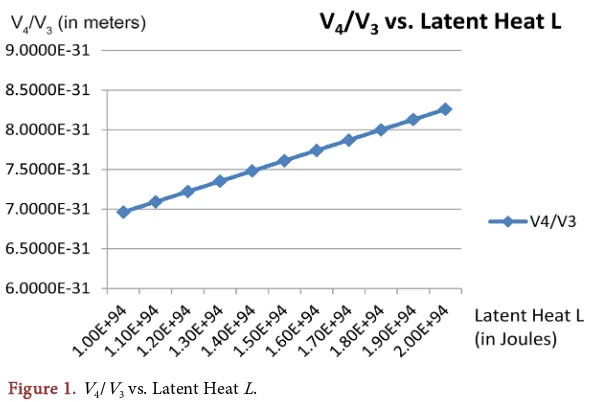
V V = × − × +L × − (3-12) A plot of V V4 3 versus L is illustrated in Figure 1, for various L values. The li-nearity is apparent. For L=0, we obtain V V₄ ₃ =5.666 10× −31m. Moreover, if L

assumes a very large value, such as 1 × 10100_{Joules, then we find correspondingly,}

that 25

4 3 1.297 10 m

V V = × − . Utilizing Equation (3-12), we can assume any val-ue for latent heat and find the corresponding ratio of volumes.

4. Inflation as a n = 4 to n = 3 Phase Transition

[image:12.595.226.527.523.724.2]

Inflation is needed in order to explain the relative homogeneity in temperature found in the very early universe, as well as the slight inhomogeneity. The un-iverse underwent a phase transition where there was rapid a-causal exponential expansion of the universe. The theory invokes a scalar field, the inflaton field, which drives this expansion. In the introduction, we discussed a heat engine model for the universe, where inflation is treated somewhat differently. It was identified with an initial isothermal expansion phase, where the expansion was

(13)

not as drastic, where there was no inflaton field, and where heat input from sur-roundings to system drove the process. In this model for inflation, the 3-d vo-lume increased by a factor of only 5.65. In this paper, we entertain the notion that the heat input needed is produced by a spatially changing phase transition. This is an alternative model, or perhaps complementary model, to heat input flowing from surroundings to system. We speculate that inflation is still an iso-thermal transition, but what provides the impetus for initiation of the heat cycle is a n=4 to

(

n− =1

)

3 change in space dimension. There is a substantial

amount of heat released in such a transition as was demonstrated in the previous section. The energy densities and entropy were also significant. This may be an alternative or complementary source of heat to drive the inflation process, in our view.

The inhomogeneity in temperature found in the WMAP and Planck satellite data, of the order of 5

5 10

T T

δ _{= ± ×} − _{, is thought to have produced during this}

inflationary period. These thermal fluctuations were due to quantum mechanical effects, radiative corrections induced by virtual particle creation and annihila-tion. The point is that they were heat driven, and since our thermodynamic va-riables depend critically on temperature, a natural question to ask is how do the thermodynamic quantities, introduced previously, depend on these thermal per-turbations? Moreover, what happens to these fluctuations if a spatially changing phase transition takes place? These are the questions, which we will address in this section.

Quite generally, given the fact that the thermodynamic variables for radiation depend strictly on temperature and dimension of space, we can vary each ther-modynamic quantity with respect to temperature. We start with the internal energy density, Equation (2-1). Varying this with respect to temperature, we find that

(

1

)

n n

u u n T T

δ = + δ _(4-1)

Similarly, using Equation (2-2), we can further claim that

(

1

)

,

(

1

)

,

n n n n n n

f f n T T p p n T T s s n T T

δ = + δ δ = + δ δ = δ _(4-2)

From these relations, we see that the dimensionality of space plays a role in determining how the thermodynamic entity responds to a relative fluctuation in temperature. In addition, quite generally, we will assert that, if the process is adiabatic in n-space, then

n n

V V n T T

δ = − δ _(4-3)

We will be assuming that a change in cosmic scale parameter in any dimen-sion “n” is inversely proportional to temperature. Just as a=R R0=T T0 holds in 3-d space, we are claiming that in n-dimensional space,

0 0

n n n

a =R R =T T (4-4)

provided we have adiabatic expansion in that n-space. In Equation (4-4), Rn is

(14)

base-DOI: 10.4236/jhepgc.2019.52016 304 Journal of High Energy Physics, Gravitation and Cosmology

line radius in that same space. Rn0 corresponds to T0 whereas Rn

corres-ponds to T. The “an” is chosen such that, at temperature T=T0, we have

0n 1

a = .

To prove Equation (4-3), we notice that Equation (2-3) allows us to express the hypervolume as n

n n

V =CR where C is some constant of order unity. There-fore, n1

n n n

V nCR R

δ ₌ −δ _and

n n n n

V V n R R

δ = δ _{. Next, we utilize Equation (4-4),} which holds only for adiabatic expansion, and write δRn Rn = −δT T.

Substi-tuting this into our expression for δV Vn n gives δV Vn n = −n T Tδ , which is

our Equation (4-3).

With Equation (4-3), we can demonstrate that

(

1

)

n n n n n

n n n n

n

U u V u V

n u V T T nu V T T

U T T

δ

= +

= + −

=

(4-5)

Therefore, δU Un n =δT T. Similarly, we find for any value of “n”,

(

p V_n _n

) (

p V_n _n

)

T T, S_n S_n 0

δ =δ δ = _(4-6)

We also recognize from Equation (2-22), and Equation (4-6b), that δ

(

L T

)

must equal zero. Therefore, it follows that

L L T T

δ =δ _(4-7)

This equation tells us that temperature fluctuations produce proportional la-tent heat fluctuations within a specified region of space. The relations, Equations (4-5)-(4-7), do not depend explicitly on spatial dimension. They do assume adiabatic expansion on both sides of the transition curve.

The conservation of energy, Equation (2-19), can be written in the simplified form, Equation (2-21). Employing Equation (4-5) and Equation (4-7), it is ob-vious that from Equation (2-21),

(

)

(

)

1

2_ n+1 n_δU_n =2_n n−1 _δU_n₋ +δL

(

)

{

(

)

1

}

2 n+1 n U n

δ

T T= 2n n−1Un− +L

δ

T T (4-8)

This equation shows that for adiabatic expansion or contraction between two neighboring spaces, any spatial temperature fluctuations carry through undimi-nished from one space to the next. Therefore, if we consider a n=4 to

(

n− =1

)

3 transition, a spatial fluctuation in temperature in

(

n− =1

)

3 space

transfers over into n=4 space. Equation (4-3) was critical in establishing

Equ-ation (4-8). Moreover, EquEqu-ation (4-3) depended in turn on relEqu-ation (4-4). What happens, however, if, in n-dimensional space and in its neighboring

(

n−1

)

space, we do not have adiabatic expansion or contraction? For example,

(15)

anywhere within that time, then we cannot assume that Equation (4-4) holds. In this instance, we claim that thermal fluctuations could have been created or produced within the transition itself.

To demonstrate this, let us assume a n=4 to

(

n− =1

)

3 transition. We

specialize Equation (2-21) to this situation, and vary that equation. We find that

4 3

10 4δU =8 3δU +δL (4-9)

We divide the left hand side of this equation by the left hand side of Equation (2-21) and we do the same on the right hand side. In this way we obtain after some algebraic manipulation

(

) (

)

(

) (

)

4 4 3 3

3 3 3 3

8 3 8 3

3 8 1 3 8

U U U L U L

U U L U L U

δ δ δ

δ δ

= + +

= + + (4-10)

For δU U3 3, we substitute δT T because of Equation (4-5). We are assum-ing that in 3-d space, after point “b” in the cycle, we do have adiabatic expansion. This gives

(

) (

)

4 4 3 3 3 8 3 1 3 8 3

U U U U L U L U

δ = δ + δ + _(4-11)

Furthermore, let us assume that δU U4 4 =0. This would mean a perfectly smooth spatial internal energy distribution, as well as total energy distribution in the originating 4-space, with absolutely no temperature perturbations. With this assumption, both the left and the right hand sides of Equation (4-11) equal zero, and we’re left with

3

3 8

T T L U

δ = − δ _(4-12) Finally, we substitute some numerical values for the quantities in Equation (4-12). For δT T, we take ±5 × 10−5, and for U3 let us use the value indicated by (3-6a). In Equation (4-12), these values give

90

/ 2.185 10 Joules

L

δ = − + × _(4-13)

The δL is defined in 3-d space and it is a small thermal perturbation when compared with 94

1.8 10 J

L= × . See Equation (3-10). From Equation (4-12), it is clear that an increase in temperature for the photons in a spatial pocket leads to a decrease in latent heat in that region. The converse holds, i.e. a decrease in temperature for photons spatially will produce an increase in latent heat in that particular region of space. This is opposite to what we had previously, for neighboring spaces where adiabatic expansion/contraction holds in each space on either side of the transition curve.

(16)

5. Summary and Conclusions

We have generalized the Clausius-Clapeyron (CC) relation to take into account a type of phase transition for which there is a change in spatial dimension. In going from n-dimensional space to

(

n−1

)

-dimensional space we have a release

of latent heat, a decrease in entropy, a decrease in energy density, and a change in volume from Vn to Vn−1. In transitioning from

(

n−1

)

dimensions in space to n dimensions, latent heat is absorbed, with an accompanying increase in en-tropy, energy density, and a change in volume from Vn−1 to Vn. The

generaliza-tion can be written as Equageneraliza-tion (2-12) where the factor of 1/2 is needed in order to retain the identity of photons in both spaces. In transitioning between spatial dimensions, total energy is conserved. See Equation (2-19). Another way to write Equation (2-19) is either Equation (2-21) or (2-22). The volume also changes from n-space to

(

n−1

)

-space, and vice versa, according to Equation (2-26), or

Equation (2-27), depending on whether we wish to work with latent heat density or latent heat.

We considered the particular phase transition from n=4 to

(

n− =1

)

3. To

give a specific example for how the generalized CC relation works, we assumed a specific value for transition temperature, as well as a particular value for latent heat. We then calculated particular values for the internal energy density, entro-py density, and volume both before and after the phase transition. We found that if we assume that 27

43 34 3 10

T =T =T = × Kelvin, and, furthermore, if we take L to equal 1.8 × 1094_{Joules, then we have:}

125 4

4 1.15 10 J m

u = × ⋅ − , 97 4 1

4 4.81 10 J m K

s = × ⋅ − ⋅ − , 31 4

4 2.14 10 m

V = × − ,

with

94 3

3 6.13 10 J m

u = × ⋅ − , s₃=2.72 10× 67J m⋅ −3⋅K−1, V₃=0.267 m3

The subscripts 3, 4 refer to the dimension of space where the quantity is de-fined. We have considered only black-body photon radiation in order to keep the discussion simple. We notice a tremendous decrease in entropy in transi-tioning from n=4 to

(

n− =1

)

3 space, as well as a dramatic change in

vo-lume. The volume V4 is defined in 4-space whereas V3 is a three-dimensional construct; as such they cannot readily be compared. Nevertheless, V3 is a sub-space of V4 because compactification will curl up one of the space dimensions. We remark that the latent heat released was assumed substantial, and we believe that it is released in the residual n=3 space as we discount exotic scenarios

such as parallel universes.

The 4-volume, V4, can be calculated once the latent heat, L, is known and vice versa. We assume that the V3 value is known since the cosmic scale para-meter is determined by the temperature, and the temperature is specified. The

3

V value at transition temperature T34=T43 must be equal to

3 3 0

V =V a− where “a” is the cosmic scale parameter, and V₀ is the present size of the

ob-servable universe. Since a=T T0 43 where T0 =2.725 K, and since the radius of the observable universe is, at present, 4.4 × 1026_{meters, we calculate for}

3

(17)

value of 0.267 m3_{at a temperature of} 27 43 3 10 K

T = × . The relation between V₄

and latent heat, L, is a linear relation with an increase in L leading to an increase in V4. See Equation (3-12), or what is equivalent, Equation (3-11). A graph for

4 3

V V versus L, for various L values, is illustrated in Figure 1.

The numbers calculated above have a direct connection to a previous work by the author [11] on inflation. We treated inflation as an isothermal expansion process, within a greater Carnot heat engine cycle. We hypothesize in this paper that the beginning of the isothermal process may have started with a n=4 to

(

n− =1

)

3 phase transition. This would account for the tremendous amount of

heat release, which is needed for the isothermal process, from points

a

→

b

in

the cycle. While this is conjecture, the numbers are seen to have the right order of magnitude. In addition, when we focus on the inhomogeneity in temperature in WMAP and Planck maps, which is of the order of 5

5 10

T T

δ _{= ± ×} − _{, we find}

that the temperature fluctuations can be produced from one spatial dimension to the next when transitioning between spaces. See, for example, Equation (4-12) and Equation (4-13). If both neighboring spaces allow for adiabatic expan-sion/contraction, then there will be a smooth carry-over of temperature inho-mogeneity from one spatial dimension to the next. This seems to be a special feature of our generalized CC relation. The specific thermodynamic variables vary in a characteristic way with respect to a variation in temperature. See Equa-tion (4-1), EquaEqua-tion (4-2). If we assume adiabatic expansion or adiabatic con-traction in n-dimensional space, then we have the further relations, Equations (4-3)-(4-7).

Higher order spatial phase transitions can be considered, e.g. from n=5 to

(

n− =1

)

4, from n=6 to

(

n− =1

)

5, etc. We can apply the generalized CC

relation, Equation (2-12), to these situations. If we multiply Equation (2-12) by negative one, left and right hand sides, we can also transition in reverse, from

(

n−1

)

spatial dimensions to n-spatial dimensions. Now latent heat must be

supplied for the process to happen, as entropy will increase as well as internal energy density.

If we decrease the number of spatial dimensions, then we can only transition from n=3 to

(

n− =1

)

2, and from n=2 to

(

n− =1

)

1. We notice that the

internal energy density, specified by Equation (2-1), is infinite for n=0 as we

are then dividing by Γ

( )

0 , which is in the denominator and is zero. If n=1 is

substituted in Equation (2-1), then the denominator is well defined, but we obtain a zero value in the numerator. Radiation energy cannot exist in a 1-dimensional space. Nevertheless, a transition from n=2 to

(

n− =1

)

1 is a possibility. As

the dimension decreases, there is less latent heat released, and the energy densi-ties decrease as well. The entropy also decreases, as more space allows for more disorder, and less space means less disorder.

(18)

in the radiation itself, i.e. within the photons, within a given dimension. What we have shown in this work is that if one gives up space, by decreasing the di-mension, one automatically releases latent heat. When one adds space, by in-creasing the spatial dimension, then one has to necessarily supply latent heat. Therefore, space itself must have energy content since transitioning between spaces supplies or costs energy. In other words, the latent heat supplied can be either positive or negative depending on the direction of the spatial transition. We can quantify the amount of energy released and taken in, when switching from one spatial dimension to another, with our generalized CC relation. This is the most spectacular result of this paper.

The author would like to thank Gonzaga University, and the Physics Depart-ment, in particular, for their support and encouragement. Special thanks goes to Dr. Eric Aver and Dr. Adam Fritsch for reading the manuscript, and offering advice. I also thank John Krehbiel for many insightful discussions. Any short-comings, however, are entirely those of author.

Conflicts of Interest

The author declares no conflicts of interest regarding the publication of this paper.

References

[1] Wark, K. and Richards, D. (2001) Thermodynamics. 6th Edition, McGraw-Hill, Inc., New York, NY.

[2] Çengel, Y.A. and Boles, M.A. (2019) Thermodynamics—An Engineering Approach. McGraw-Hill Series in Mechanical Engineering. 9th Edition, McGraw-Hill, Inc., Boston, MA.

[3] Salzman, W.R. (2001) Clapeyron and Clausius-Clapeyron Equations. Chemical Thermodynamics. University of Arizona,Tucson.

[4] Krafcik, M. and Sánchez Velasco, E. (2014) Beyond Clausius-Clapeyron: Determin-ing the Second Derivative of a first-Order Phase Transition Line. American Journal of Physics, 82, 301-305.

[5] Klein, O. (1926) Quantentheorie und fünfdimensionale Relativitätstheorie. Zeit-schrift für Physik A, 37, 895-906.

[6] Jordan, P. (1948) Fünfdimensionale Kosmologie. Astronomische Nachrichten, 276, 193-208.

[7] Appelquist, T., Chodos, A. and Freund, P.G.O. (1987) Modern Kaluza-Klein Theo-ries. Addison-Wesley, Menlo Park.

[8] Wesson, P.S. (1999) Space-Time-Matter, Modern Kaluza-Klein Theory. World Scien-tific, Singapore. https://doi.org/10.1142/3889

[9] Wesson, P.S. and Ponce de Leon, J. (1995) The Equation of Motion in Kaluza-Klein Cosmology and Its Implications for Astrophysics. Astronomy and Astrophysics, 294, 1-7.

[10] Castellani, L., et al. (1991) Supergravity and Superstrings. Vol. 2, Chapter V.11, World Scientific Publishing, Singapore.

(19)

DOI: 10.4236/jhepgc.2019.52016 309 Journal of High Energy Physics, Gravitation and Cosmology [12] Kolb, E. and Turner, M. (1994) The Early Universe.

[13] Mather, J.C., et al. (1999) Calibrator Design for the COBE Far-Infrared Absolute Spectrophotometer (FIRAS). The Astrophysical Journal, 512, 511-520.

https://doi.org/10.1086/306805

[14] Husdal, L. (2016) On Effective Degrees of Freedom in the Early Universe. ar-Xiv:1609.04979v3.

[15] Gonzalez-Ayala, J., Cordero, R. and Angulo-Brown, F. (2016) Is the (3+1)-d Nature of the Universe a Thermodynamic Necessity? EPL (Europhysics Letters), 113, 40006.

[16] Landsberg, P.T. and De Vos, A. (1989) The Stefan Boltzmann Constant in an N-Dimensional Space. Journal of Physics A: Mathematics and General, 22, 1073-1084.https://doi.org/10.1088/0305-4470/22/8/021

[17] Menon, V.J. and Agrawal, D.C. (1998) Comment on “The Stefan-Boltzmann Con-stant in N-Dimensional Space”. Journal of Physics A: Mathematics and General, 31, 1109-1110.https://doi.org/10.1088/0305-4470/31/3/021

[18] Barrow, J.D. and Hawthorne, W.S. (1990) Equilibrium Matter Fields in the Early Universe. Monthly Notices of the Royal Astronomical Society, 243, 608-609. [19] Gonzalez-Ayala, J., Perez-Oregon, J., Cordero, R. and Angulo-Brown, F. (2015) A

Possible Cosmological Application of Some Thermodynamic Properties of the Black Body Radiation in N-Dimensional Euclidean Spaces. Entropy, 17, 4563-4581.

https://doi.org/10.3390/e17074563

[20] Equation 5.19.4, NIST Digital Library of Mathematical Functions.

https://dlmf.nist.gov/5.19#iii

[21] Wang, X. (2005) Volumes of Generalized Unit Balls. Mathematics Magazine, 8, 390-395.https://doi.org/10.2307/30044198

[22] Frequently Asked Questions in Cosmology. Astro.ucla.edu.