graphical convolution , determine the output for

ECE 300

Signals and Systems

Homework 4

Due Date: Tuesday September 26 at 2:30 PM Exam #1, Thursday September 21.

Problems

1. K & H, Problem 2.29 parts a,c, and e. Do these convolutions graphically. You only need to plot the results for part a.

2. (From a previous exam) Consider a causal linear time invariant system with impulse response given by

( 1) ( ) t ( 1) h t =e− − u t−

The input to the system is given by

( ) ( ) ( 1) ( 3)

x t =u t −u t− +u t−

Using graphical convolution, determine the outputy t( ) for 2≤ ≤t 5. Note the limited range of t we are interested in !

Specifically, you must

a) Flip and slideh t( )

b) Show graphs displaying both h t( −λ) and x( )λ for each region of interest c) Determine the range of t for which each part of your solution is valid d) Set up any necessary integrals to compute y t( )

e) Evaluate the integrals

You should get (in unsimplified form)

( 1) 1

( 1) 1 ( 1) 1 3

[ 1] 2

( )

[ 1] [ ] 4

t

t t t

e e t

y t

e e e e e t

− −

− − − − −

⎧ 4

5

− ≤ ≤

= ⎨

− + − ≤

⎩ ≤

3. (From a previous final exam) Consider a linear time invariant system with impulse response given by

( 1) ( ) t ( 1) h t =e− + u t+

The input to the system is given by

( ) 2[ ( ) ( 1)] 3[ ( 3) ( 4)]

x t = u t −u t− + u t− −u t−

Using graphical convolution, determine the outputy t( ). Specifically, you must a) Flip and slideh t( )

b) Show graphs displaying both h t( −λ) and x( )λ for each region of interest c) Determine the range of t for which each part of your solution is valid d) Set up any necessary integrals to compute y t( ) Do Not Evaluate the Integrals

4. Pre-Lab Exercises (to be done by all students. Turn this in with your homework and bring a copy of this with you to lab! Yes, it counts towards both grades!)

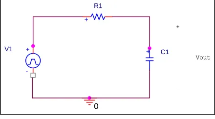
a)Calculate the impulse response of the RC lowpass filter shown in Figure 1, in terms of unspecified components R and C. Determine the time constant for the circuit.

+

C1

Vout

-+

0 +

-V1

+ R1

Figure 1. Simple RC lowpass filter circuit.

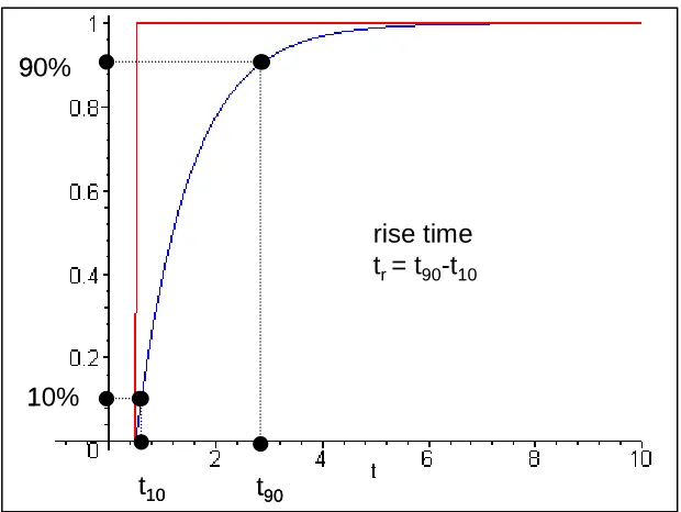
b) Find the step response of the circuit, and determine the 10-90% rise time. , as shown below in Figure 2. The rise time is simply the amount of time necessary for the output to rise from 10% to 90% of its final value. Specifically, show that the rise time is given by

r t

ln(9) r

t90 t₁₀

rise time tr= t90-t10 90%

10%

t90 t₁₀

rise time tr= t90-t10 90%

10%

Figure 2. Step response of the RC lowpass filter circuit of Figure 1, showing the definition of the 10-90% risetime.

c) Specify values R and C which will produce a time constant of approximately 1 msec. Be sure to consider the fact that the capacitor will be asked to charge and discharge quickly in these measurements.

d) Show that the response of the circuit to a unit pulse of length T (, i.e. a pulse of amplitude 1 starting at 0 and ending at T) is given by

/ ( ) /

( ) (1 t ) ( ) (1 t T ) ( ) pulse

y t = −e− τ u t − −e− − τ u t T−

e) Plot the response to a unit pulse (in Matlab) for τ =0.001 and , 0.001, and 0.0001 from 0 to 0.008 seconds. Note on the plots the times the capacitor is charging and discharging. Use the subplot command to make three separate plots, one on top of another (i.e., use subplot(3,1,1), subplot(3,1,2),

subplot(3,1,3)).

0.003 T =

f) If the input is a pulse of amplitude A and width T, determine an expression for

the amplitude of the output at the end of the pulse, y_pulse( )T . Assume that T 1

τ

5. (Matlab Problem) Read the Appendix, then

a) Open an m-file named Fourier_Sine_Series.m and type the code in the appendix into the file. Think about what you are doing as you do this!

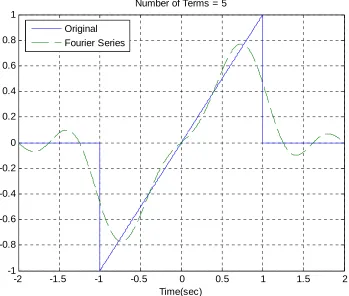
b) If you type (in Matlab’s command line) Fourier_Sine_Series(5) you should get a plot like that shown in Figure 3. As you increase the number of terms in the Fourier series, you should get a better match to the function. Run the code for N=100 and turn in your plot.

c) Copy Fourier_Sine_Series.m to a file named Trig_Fourier_Series.m and implement a full trigonometric Fourier series representation. This means you will have to compute the average value and the , and then use these values in the final estimate.

o

a a_k

d) Using the code you wrote in part c, find the trigonometric Fourier series representation for the following functions (defined over a single period)

1( ) ( ) 0 3

t

f t =e u t− ≤ <t

2

0 2

( ) 3 2 3

0 3 4

t t

f t t

t ≤ < ⎧

⎪

=_⎨ ≤ < ⎪ _{≤ <} ⎩

3

0 2

1 1 2

( )

3 2 3

0 3 4

t t f t

t t

1 − ≤ < − ⎧

⎪ _{− ≤ <} ⎪

= ⎨ _{≤ <} ⎪

⎪ _{≤ <} ⎩

-2 -1.5 -1 -0.5 0 0.5 1 1.5 2 -1

-0.8 -0.6 -0.4 -0.2 0 0.2 0.4 0.6 0.8 1

Time(sec) Number of Terms = 5 Original

Fourier Series

Figure 3. Trigonometric Fourier series for problem 4b.

Appendix

In DE II you learned about representing periodic functions with a Fourier series using trigonometric functions (sines and cosines). In this appendix we will determine how to determine a Fourier sine series series for an odd periodic function using our knowledge of numerical integration in Matlab. The only new thing we will need is the idea of a loop.

Trigonometric Fourier Series If x t( ) is a periodic function with fundamental period T, then we can represent x t( ) as a Fourier series

0

1 1

( ) _kcos( _o ) _ksin( )

k k

o

x t a a kω t b kω t

∞ ∞

= =

= +

∑

∑

0 0 0 1 ( ) 2

( ) cos( ) 2

( ) sin( ) T o T k o T k o

a x t dt

T

a x t k t

T

b x t k t

T ω ω = = =

∫

∫

∫

Even and Odd Functions Recall that a function x t( ) is even if x t( )= −x( t) (it is symmetric about the y-axis) and is odd if x(− = −t) x t( )(it is antisymmetric about the y-axis). If we know in advance that functions are even or odd, we can determine that some of the Fourier series coefficients are zero. Specifically,

Ifx t( ) is even all of the b_k are zero.

Ifx t( ) is odd all of the a_k (including a_o) are zero.

For Loops Let’s assume we want to generate the coefficients ₂

1 k k b k =

+ for k =1

to k=10. One way of doing this in Matlab is by using the following for loop for k=1:10

b(k) = k/(1+k^2); end;

In this loop, the variable k first takes the value of 1 until the end is reached, then the value 2, all the way up to k = 10. In this loop we are assigning the coefficients to the array b, hence b(1) = , b(2) = b₁ b₂, etc.

Similarly, if we wanted to generate the coefficients 1

1 k

a k =

+ and 2

2 1 k b k =

+ for

to , we could do this using for loops as follows:

1

k= k=5

for k=1:5

a(k) = 1/(k+1); b(k) = 2/(k^2+1); end;

Note that Matlab requires the indices in an array to start at 1, and that for loops should usually be avoided in Matlab if possible since they are usually less efficient (Matlab is designed for vectorized operations).

0 2

( ) 1 1

0 1 2

t

x t t t

t 1 − ≤ < − ⎧

⎪

=_⎨ − ≤ < ⎪ _{≤ <} ⎩

This is clearly an odd function, so we will only need to generate a Fourier sine series. The following program will generate the required Fourier sine series:

%

% This routine implements a trigonometric Fourier Sine Series %

% Inputs: N is the number of terms to use in the series %

function Fourier_Sine_Series(N) %

% one period of the function goes from low to high %

low = -2; high = 2; %

% the difference between low and high is one period %

T = high-low; w0 = 2*pi/T; %

% the periodic function... %

x = @(t) 0.*(t<-1) + t.*((-1<=t)&(t<1)) + 0.*(t>=1); %

% find b(1) to b(N) %

for k = 1:N

arg = @(t) x(t).*sin(k*w0*t); b(k) = (2/T)*quadl(arg,low,high); end;

%

% determine a time vector over one period %

t = linspace(low,high,1000); %

% find the Fourier series representation %

est = 0; for k=1:N

est = est + b(k)*sin(k*w0*t); end;

%