arXiv:0904.4575v3 [hep-th] 24 Sep 2009
Preprint typeset in JHEP style - HYPER VERSION ITP-UU-09-17 SPIN-09-17 TCDMATH-09-12 HMI-09-06
The Dressing Factor and Crossing Equations
Gleb Arutyunova∗†and Sergey Frolovb†
a Institute for Theoretical Physics and Spinoza Institute,
Utrecht University, 3508 TD Utrecht, The Netherlands
b Hamilton Mathematics Institute and School of Mathematics,
Trinity College, Dublin 2, Ireland
Abstract: We utilize the DHM integral representation for the BES dressing factor
of the world-sheet S-matrix of the AdS5×S5 light-cone string theory, and the crossing
equations to fix the principal branch of the dressing factor on the rapidity torus. The results obtained are further used, in conjunction with the fusion procedure, to determine the bound state dressing factor of the mirror theory. We convincingly demonstrate that the mirror bound state S-matrix found in this way does not depend on the internal structure of a bound state solution employed in the fusion procedure. This welcome feature is in perfect parallel to string theory, where the corresponding bound state S-matrix has no bearing on bound state constituent particles as well. The mirror bound state S-matrix we found provides the final missing piece in setting up the TBA equations for the AdS5×S5 mirror theory.
∗Email: [email protected], [email protected]
Contents
1. Introduction 1 2. The dressing phase and crossing equations 5
2.1 Uniformization tori 5
2.2 Dressing and crossing for fundamental particles 6 2.3 Dressing and crossing for bound states 9
3. Φ- and Ψ-functions 9
3.1 Φ-function 10
3.2 Ψ-function 10
3.3 Functionχ for |x1| ≈1,|x2| ≈1 14
4. The dressing phase for fundamental particles 16 4.1 Analytic continuation of the dressing phase 16 4.2 The crossing equations for fundamental particles 22
5. Bound state dressing factor of string theory 23 5.1 Analytic continuation of the bound state dressing phase 23 5.2 The crossing equations for bound states 31
6. Bound state dressing factor of mirror theory 33 7. Conclusions 37 8. Appendix 38 8.1 Some results on the dressing phase for fundamental particles 38
8.2 Identities for the Ψ-function 40
8.3 An alternative derivation of the dressing factor 41 8.4 Details on the derivation of the mirror bound state dressing factor 43
1. Introduction
The exact finite-size spectrum of the AdS5×S5 superstring remains one of the most
proportional to the light-cone momentum. When the light-cone momentum tends to infinity, the string world-sheet decompactifies and, under the assumption of quantum integrability of the light-cone model, one can apply factorized scattering theory [2] and the Bethe ansatz to capture the spectrum. A lot of remarkable progress has been achieved in this way, for the recent reviews and extensive list of references, see, e.g. [3]-[5].
On the infinite world-sheet the string sigma model exhibits massive excitations which transform in the tensor product of two fundamental representations of the
psu(2|2) superalgebra enhanced by two central charges, both dependent on the
gen-erator of the world-sheet momentum [6, 7]. The symmetry algebra severely constrains the matrix form of the two-particle S-matrix [6] and, together with the Yang-Baxter equation and the requirement of generalized physical unitarity [8, 9], leads to its unique determination up to an overall scalar function of particle momenta. This func-tion includes, as its most non-trivial piece, the so-called dressing factor σ= exp(iθ), where θ is the dressing phase [10]. Taking into account that the light-cone S-matrix is compatible with the assumption of crossing symmetry, one finds that the latter implies certain functional relations for the dressing factor, known as the crossing equations [11]. A solution to these equations has been found in the strong coupling expansion in terms of an asymptotic series [12]. The corresponding dressing factor appears to be compatible with all available classical and perturbative string data [10], [13]-[19] and it passed a number of further non-trivial checks, see e.g. [20, 21].
The dressing factor suitable for the weak coupling expansion has been also pro-posed by assuming a certain analytic continuation of its strong-coupling counterpart [22], and in what follows we refer to it as the Beisert-Eden-Staudacher (BES) dress-ing factor. The proposal was successfully confronted against direct field-theoretic perturbative calculations [23]-[25]. However, it has not been shown so far that the BES dressing factor satisfies crossing equations for finite values of the string coupling. Filling this gap is among the goals of this paper.
approach [9].
Recently, we have derived a set of the TBA equations for the AdS5×S5 mirror
model [29, 30]. A parallel development took place in the works [31, 32] and [33], where also the so-called Y-system has been proposed. The Y-system represents a set of local equations which is believed to contain the whole spectrum (the ground and excited states), and it is obtained from the original infinite set of TBA equations by taking a certain projection. In one respect the undertaken derivations of the mirror TBA equations and the associated Y-system remain incomplete. To completely define the TBA equations and, therefore, to make them a working device, one has to understand the so far unknown analytic properties of the dressing factor in the kinematic region of the mirror theory.
To be precise, the BES dressing phase is represented by a double series convergent in the region |x±
1| > 1 and |x±2| > 1, where x±1,2 are kinematic parameters related
to the first and the second particle, respectively. This series admits an integral representation found by Dorey, Hofman and Maldacena (DHM) [34] which is valid in the same region of kinematic parameters and for finite values of the string coupling.1
To find the BES dressing phase in other kinematic regions of interest (in the mirror region), one has to analytically continue the DHM integral representation beyond
|x±1,2|>1. Understanding this continuation is precisely the subject of this paper.
Regarding the dressing phase as a multi-valued function, we want to fix its particular analytic branch which satisfies the crossing equations. In fact, continuation compatible with crossing is the main rationale behind our treatment. Consideration of crossing requires us to associate to each of the particles (bound states) the so-called rapidity torus (the z-torus) which uniformizes the corresponding dispersion relation [11]. The analytically continued dressing phase should be then understood as a functionθ(z1, z2), wherez1 andz2 belong to the corresponding tori, see section 2
for a more precise definition. This function must satisfy the crossing equation in each of its arguments for z1, z2 being anywhere on the tori. Thus, to construct θ(z1, z2),
we choose an analytic continuation path on the z-torus which starts in the particle region, where|x±(z)|>1, and penetrates the other regions of thez-torus. Following
this path, we properly account for the change of the DHM integral representation to guarantee the continuity of our resulting function. In this way we build up the analytic continuation of the dressing phase to all possible kinematic regions and then verify the fulfillment of the crossing equations.
We further study the analytic continuation of the dressing factor for bound states of the string model. This dressing factor is obtained by fusing the dressing factors of bound state constituent particles, all of them being in the region |x±(z)|>1 of the
elementaryz-torus. The dressing factor is then analytically continued into the whole bound state z-torus in a way compatible with the corresponding crossing equations.
In view of applications to the TBA program, we also determine the dressing factor for bound states of the mirror model by fusing the dressing factors of constituent mirror particles. Since some of these particles fall necessarily outside the region
|x±(z)|>1, in the fusion procedure we use their analytically continued expressions.
Equations defining aQ-particle bound state admit 2Q−1different solutions and, since
any of these solutions can be used in the fusion procedure, this raises a question about uniqueness of the final result. To find an answer, it is important to realize that dealing with mirror TBA equations, we are mainly interested not in the bound state dressing factor σQQ′
itself but rather in the following quantity
ΣQQ′
=σQQ′
Q Y
j=1
Q′
Y
k=1
1− x+1
jzk−
1− x−1
jz
+
k
which logarithmic derivative appears as one of the TBA kernels [30]. Herex±
j andzk± are the kinematical parameters of the constituent particles corresponding toQ- and Q′-particle bound states, respectively. The improvedfactor ΣQQ′
originates from fu-sion of the scalar factors of mirror theory scattering matrices corresponding to bound state constituent particles. By evaluating ΣQQ′
on a particular bound state solution, we then show that the resulting expression depends on the bound state kinematic parameters only and that all the dependence on constituent particles completely dis-appears! This indicates that ΣQQ′
is the same for all bound state solutions, as we also confirm by explicitly evaluating it on yet another solution. In this respect ΣQQ′
appears as good as the corresponding bound state dressing factor of the original string theory. We derive an explicit formula (6.14) for ΣQQ′
which can be used to complete the mirror TBA equations.
2. The dressing phase and crossing equations
In the light-cone gauge the string sigma model exhibits a massive spectrum. The cor-responding particles transform in the tensor product of two fundamental multiplets of the centrally extended su(2|2) superalgebra. Besides the fundamental particles
the asymptotic spectrum also contains their bound states which manifest themselves as poles of the scattering matrix for fundamental particles. AQ-particle bound state [36] transforms in the tensor product of two 4Q-dimensional atypical totally sym-metric multiplets of the centrally extended su(2|2) superalgebra [37, 38]. Both the
fundamental and the bound state S-matrices are determined by kinematical symme-tries and additional physicality requirements up to an overall scalar factor. Upon normalizing the kinematically determined S-matrix in a certain (canonical) way, the corresponding scalar factor acquires an absolute meaning and therefore becomes an important dynamical characteristic of the model. For the AdS5×S5 superstring the
scalar factor is proportional to the dressing factor σ, the latter can be expanded over local conserved charges of the model [10]. By unitarity σ = exp(iθ), where θ is known as thedressing phase. This section has an introductory character, its purpose is to recall the relevant facts about the dressing phase as well as to introduce the necessary notation.
2.1 Uniformization tori
As was argued in [11], the world-sheet S-matrix appears to be compatible with an assumption of crossing symmetry that corresponds to replacing a particle for its anti-particle. Implementation of this symmetry leads to a non-trivial functional relation for the dressing phase.
Similar to the more familiar relativistic case, a rigorous treatment of crossing symmetry requires finding a Riemann surface which uniformizes the dispersion re-lation of the model. For fundamental particles this uniformization is achieved by introducing a torus with real and imaginary periods given by
2ω1 = 4K(k), 2ω2 = 4iK(1−k)−4K(k), (2.1)
respectively [11, 39] . Here K(k) stands for the complete elliptic integral of the first kind. The elliptic modulus k =−4g2, where g is the string tension related to the ‘t
Hooft couplingλ asg = √λ
2π.
Analogously, the dispersion relation corresponding to a Q-particle bound state is also uniformized by an elliptic curve whose periods are obtained by replacing in eq.(2.1) the coupling constant g with g/Q. Neglecting for the moment the dressing factor, the canonically normalized S-matrix that describes scattering of Q- and M -particle bound states turns out to be a meromorphic matrix function SQM(z1, z2)
-1 -0.5 0.5 1
-2 2 4
-1 -0.5 0.5 1
-2 2 4
+| 1
| |x 1
Ix < >
-<
| | |
| x x
+ ->11
| | | |xx
< < 1 1
+
-| -| | | x x >1
1
+
->
-1 -0.5 0.5 1
-2 2 4
Im+
0
x Imx-< 0
Imx 0
Im+
-< 0 x
Im+-< 0 x
Imx+->0 >
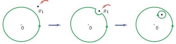
[image:7.612.130.469.83.240.2]>
Figure 1: On the left figure the torus is divided by the curves |x+| = 1 and|x−|= 1 into four non-intersecting regions. The middle figure represents
the torus divided by the curves Im(x+) = 0 and Im(x−) = 0, also in four
regions. The right figure contains all the curves of interest.
In addition, we will also need the variables x± which satisfy the following
con-straint
x++ 1 x+ −x
−− 1
x− =
2i
g (2.2)
and which are related to the torus variable z through x+
x− = exp(i2amz), where
amz is the Jacobi amplitude. The functions x±(z) are meromorphic on the z-torus
corresponding to fundamental particles. The torus itself can be divided into four non-intersecting regions in two different ways: either by curves|x±|= 1 or by curves
Imx± = 0, see Figure 1. These divisions will play an important role in our subsequent
discussion of the dressing phase.
Under the crossing symmetry transformation the variables x± undergo the
in-version: x± → 1/x±. In terms of variable z, this map is realized as a shift by the
imaginary half-period: z →z±ω2 [11]. The dressing phase, however, is not periodic
on thez-torus and should be considered as a function on the product of twoz-planes. The crossing symmetry allows one to define the dressing phase on the product of two complex planes from its knowledge on the z-torus, the latter being regarded as the fundamental domain. As we will see later on, inside this fundamental domain the dressing phase has an infinite number of cuts.
2.2 Dressing and crossing for fundamental particles
The dressing phase for fundamental particles is a function of the constrained variables x±: θ ≡θ(x+
series expansion [10, 41]
θ(x+1, x−1, x+2, x−2) =
∞
X
r=2
∞
X
s>r r+s=odd
cr,s(g)hqr(x±1)qs(x±2)−qr(x±2)qs(x±1)i, (2.3)
where the local conserved charges qr(x±) are
qr(x−
k, x
+
k) = i r−1
" 1 x+k
r−1
−
1 x−k
r−1#
. (2.4)
Here the coefficients cr,s(g) are non-trivial real functions of the string tension admit-ting a well-defined asymptotic expansion for largeg. The double series representation (2.3) implies that the dressing phase in this region can be written [42] via a single skew-symmetric function χ of two variables
χ(x1, x2) =−
∞
X
r=2
∞
X
s>r r+s=odd
cr,s(g) (r−1)(s−1)
h 1
xr−1 1 xs2−1
− 1
xr−1 2 xs1−1
i
(2.5)
as a sum of four terms θ(x+1, x−
1, x+2, x−2) = χ(x1+, x+2)−χ(x+1, x−2)−χ(x−1, x+2) +χ(x−1, x−2). (2.6)
At any given order in the asymptotic 1/g expansion the double series defining χ is convergent for |x1,2| >1. For the z-torus in Figure 1, conditions |x±(z)| > 1 single
out a green region with the shape of a “fish”. Thus, every term in the strong coupling asymptotic expansion of the dressing phase θ(z1, z2) is a well-defined function
pro-vided both z1 and z2 belong to the “fish”. The set of points on the z-torus obeying
|x±(z)|>1 will be called the particle region.
Assuming the functional form (2.3), the equations implied by crossing symmetry (to be discussed below) can be solved perturbatively in the strong coupling expansion, the coefficients cr,s(g) emerge in the form of an asymptotic series [12]. On the other hand, the coefficients cr,s(g) admit a convergentsmall g expansion
cr,s(g) =g
∞
X
n=r+s−3
gnc(r,sn).
The weak coupling coefficients c(r,sn) have been determined from their strong coupling cousins by assuming a certain analytic continuation procedure [22].
By using the weak coupling expressions for cr,s(g) and the series (2.5), in the work [34] an integral representation forχvalid for finite values ofg was obtained. It is given by the following double integral
χ(x1, x2) =i
I dw
1
2πi
I dw
2
2πi
1
(w1−x1)(w2−x2)
log Γ
1 + i
2g w1 + 1
w1 −w2−
1
w2
Γ1− i
2g w1+ 1
w1 −w2−
1
w2 ,
where integrations are performed over the unit circles. The integral representation (2.7) holds for|x1,2|>1 and, therefore, from the point of view of thez-torus, for any
finite value of g, it renders the dressing phase (2.6) a well-defined function on the product of two particle regions. We will call eq.(2.7) the DHM integral representation. Assuming that the dressing phase θ(z1, z2) is defined on the whole z-torus, the
functional equations implied by crossing symmetry read as
θ(z1, z2) +θ(z1+ω2, z2) =
1 i log
hx−
2
x+2 h(x1, x2) i
, (2.8)
θ(z1, z2) +θ(z1, z2−ω2) =
1 i log
hx+ 1
x−
1
h(x1, x2)
i
, (2.9)
where
h(x1, x2) =
x−1 −x+2 x−1 −x−2
1− x+1 1x
+ 2 1− x+1
1x−2
. (2.10)
Under the double crossing one gets, for instance,
θ(z1+ 2ω2, z2)−θ(z1, z2) =
1
i loghD(x1, x2), (2.11) where
hD(x1, x2) =
(x+1 −x+2)(x−1 −x−2) (x+1 −x−2)(x−1 −x+2)
1− 1
x−
1x + 2
1− 1
x+1x−
2
1− x+1 1x+2
1−x−1
1x−2
, (2.12)
which shows that 2ω2 is not a period of the dressing phase.
It should be stressed that so far crossing symmetry has been imposed on the dressing phase in the asymptotic sense only, and this led, through the analytic con-tinuation procedure from strong to weak coupling, to the finite g representation defined with the help of (2.7). Verification of crossing symmetry for finiteg, i.e. not in the asymptotic sense, constitutes an open problem. Its solution relies on finding an analytic continuation of the dressing phase from the particle region to the whole z-torus which is compatible with crossing symmetry.
Our final remark concerns the integral representation (2.7). Formula (2.7) holds for |x1,2| > 1 but, in fact, it can be used to continue the function χ for each of
its arguments slightly inside the unit circle. Indeed, the integration contours can be chosen to be circles of any radius r > rcr ≡
q 1 + 1
4g2 − 21g, and, therefore, the integral representation above can be extended for|x1,2|> rcr. Moreover, if one of the
2.3 Dressing and crossing for bound states
The dressing phase which describes scattering ofQ- andM-particle bound states can be obtained from the dressing phase for fundamental particles by means of the fusion procedure [43, 44]. The fused dressing phaseθQM is given by the same formulae (2.6) and (2.7), where now the variablesx±1 andx±2 are associated to theQ- andM-particle bound states, respectively
x+1 + 1 x+1 −x
−
1 −
1 x−1 =
2i
g Q , x
+ 2 +
1 x+2 −x
−
2 −
1 x−2 =
2i
g M . (2.13) The crossing equations for the dressing factor describing scattering of Q- and M-particle bound states are [40]2
σQM(z
1, z2)σQM(z1 +ω2, z2) =
x−2 x+2
Q
x−1 −x+2 x−1 −x−2
1− 1
x+1x+2 1− x+1
1x−2 Q−1
Y
k=1
G(M −Q+ 2k),
σQM(z1, z2)σQM(z1, z2−ω2) =
x+1 x−
1
M x−
1 −x+2
x−
1 −x−2
1− x+1 1x+2 1− 1
x+1x−
2 Q−1
Y
k=1
G(M −Q+ 2k), (2.14)
where the following function was introduced
G(ℓ) = u1−u2− i gℓ u1−u2+ giℓ
.
Here for a Q-particle bound state the variableu≡uQ is defined as
uQ=x++ 1 x+ −
i
gQ=x
−+ 1
x− +
i gQ .
Taking the logarithm of both sides of eqs. (2.14), one obtains the corresponding equa-tions for the dressing phase. As for the case of fundamental particles, the dressing phase describing scattering of bound states is a well-defined function in the particle region of the z-torus and it should be analytically continued to the whole torus in a way compatible with crossing equations (2.14).
3.
Φ
- and
Ψ
-functions
In this section we introduce Φ- and Ψ-functions and discuss the analytic continuation of χ in terms of these functions for x1, x2 close to the unit circle.
2The second formula in (2.14) follows from the first one by using the unitarity condition σQM(z
1, z2)σM Q(z2, z1) = 1, and the identityQMk=0−1G(Q−M+ 2k) = QQ−1
3.1 Φ-function
Let us introduce a function Φ(x1, x2) defined as the following double integral of the
Cauchy type
Φ(x1, x2) =i
I dw1
2πi I
dw2
2πi
1
(w1−x1)(w2−x2)
log Γ
1 + i
2g w1+ 1
w1 −w2−
1
w2
Γ1− i
2g w1+ 1
w1 −w2−
1
w2
,(3.1)
where the integrals are over the unit circles. Since the integrand is a continuous function of ϑ1, ϑ2 where wi = eiϑi, the function Φ is unambiguously defined by this
integral formula for all values of x1, x2 not lying on the unit circle.
Ifx1(orx2 or both) is on the unit circle, we can define Φ(eiϕ1, x2) as the following
limit
Φ(eiϕ1, x
2)≡ lim
ǫ→0+Φ(e
ǫeiϕ1, x
2), (3.2)
i.e. we approach the value x1 = eiϕ1 from exterior of the circle. This limit exists
because for |x1| >1, |x2| 6= 1, and |w2|= 1 the integrand in (3.1) is a holomorphic
function of w1 in the annulus
q
1 + g12 −1g <|w1|<|x1|.
If we would define the limiting value of Φ by approaching x1 = eiϕ1 from the
interior of the circle we would obtain the result different from (3.2) and, for this reason, the function Φ is not continuous across|x1|= 1. In fact, it is not difficult to
see that
lim ǫ→0+Φ(e
−ǫ eiϕ1, x
2) = Φ(eiϕ1, x2) + (3.3)
+i I
dw 2πi
1 w−x2
logΓ
1 + i
2g 2 cosϕ1−w− 1
w
Γ1− i
2g 2 cosϕ1−w− 1
w .
The function Φ is skew-symmetric Φ(x1, x2) = −Φ(x2, x1), and it also satisfies the
following important relation
Φ( 1 x1
, x2) + Φ(x1, x2) = Φ(0, x2), |x1| 6= 1, (3.4)
which will be used to prove the crossing equations for the dressing phase. If|x1| = 1
this relation is modified in an obvious way due to eq.(3.3).
3.2 Ψ-function
The formula (3.3) suggests to introduce the following function
Ψ(x1, x2) = i
I dw 2πi
1 w−x2
log Γ
1 + i
2g x1+ 1
x1 −w−
1
w
Γ1− i
2g x1+ 1
x1 −w−
1
w
which is equal to the second term in (3.3) forx1 =eiϕ1. By construction, Ψ(x1, x2) =
Ψ(1/x1, x2). Ifx1 is close enough to the unit circle then the function Ψ(x1, x2) is
well-defined for all |x2| 6= 1, and if |x2| = 1 we obviously can use the same prescription
(3.2),i.e. we approachx2 =eiϕ2 from exterior of the unit circle. This representation
for Ψ will apparently break down for such values ofx1 for which the arguments of the
Γ-functions in (3.5) become negative integers for somewon the integration contour. To analyze this situation in the case|x2| >1, it is convenient to integrate (3.5)
by parts obtaining the following expression
Ψ(x1, x2) =−
g 2
I dw
2πilog(w−x2)
1− 1 w2
(3.6)
×
ψ1 + i
2g x1 + 1 x1 −
w− 1 w
+ψ1− i
2g x1+ 1 x1 −
w− 1 w
,
where the cut of the log-function should not intersect the unit circle.3 Then, instead
of dealing with the cuts of log Γ-functions, we analyze the location of poles of the ψ-functions, cf. [34].
We use formula (3.6) as the definition of the function Ψ(x1, x2) for|x2|>1 and
for all values of x1 where the integral representation is well-defined. This defines Ψ
as an analytic function on the x1-plane with cuts. To determine the location of the
cuts, we first notice that for a generic value ofx1 none of the infinitely many poles of
the ψ-functions in thew-plane falls on the unit circle. If we now start continuously changing x1, the poles start to move. At a certain pointx1 might become such that
two poles of one of the ψ-functions in eq.(3.6) reach the circle. The values of x1 for
which this happens are solutions to the following equations
x1+
1 x1 −
w− 1 w =
2i
gn , n ≥1, (3.7)
w+ 1
w −x1− 1 x1
= 2i
gn , n ≥1, (3.8)
where w is on the unit circle: w = eiθ. Solutions of (3.7) and (3.8) correspond to poles of the first and second ψ-functions in (3.6), respectively. It is clear that if x1
and θ solve one of these equations then x1 and −θ also do. Thus, for each x1 there
are two values of θ, and two poles of one of the ψ-functions are on the unit circle. Equations (3.7) and (3.8) can be solved in terms of the following function x(u)
x(u) = u 2 1 +
r 1− 4
u2
!
, (3.9)
3In Mathematica one could use
log(w−x)→itan−1w−Re(x)
Im(x)
+1
2log w
2−2Re(x)w+ Im(x)2+ Re(x)2
1.0 0.5 0.5 1.0
1.0 0.5 0.5 1.0
x(n )+
[image:13.612.235.362.81.211.2]x(n )+ x(¡n) x(¡n)
Figure 2: The curves x(±n) = 1/x(u±2gin) with −2 ≤u=w+ w1 ≤2 for g= 3 and n= 1,2,3,4. The endpoints of the curves correspond to w=±1. The curves closest to the circle correspond to n= 1.
where the cut ofx(u) is from −2 to 2. The functionx(u) maps the complexu-plane with the cut [−2,2] onto exterior of the unit circle, i.e. |x(u)| > 1 for any u. We are interested in solutions with |x1|<1 because we will be using the Ψ-function to
define the dressing phase in this region. Then the solutions to (3.7) and (3.8) take the following form
x(±n)(u) = 1 x(u± 2i
gn)
, u=w+ 1
w, −2≤u≤2, (3.10)
where the + sign is for the solution to eq.(3.7). It is clear that all solutions to eqs.(3.7) and (3.8) lie in the lower and upper half-circles, respectively, because Imx(u+iy)>0 and Imx(u−iy)<0 for y >0.
Further, we point out that eqs.(3.7) and (3.8) can be thought of as the constraint equations for xn± parameters of n-particle bound states, and the general solutions
to these equations can be written as
x(+n) =xn+(z), w=xn−(z) =eiθ, (3.11) x(−n) =xn−(z), w=xn+(z) =eiθ. (3.12)
The function Ψ is obviously discontinuous across any curve x(±n). However, for
|w|= 1 the curves x(±n) are not closed4 in the x-plane, and, therefore, one can always
reach any point inside the unit circle without crossing them, see Figure 2. Thus, the curves x(±n) represent the cuts of Ψ. In general, one should think of Ψ as being an analytic function (for |x2| > 1) on an infinite genus surface. Specifying the cut
structure as described above, defines its particular branch, that we will be using in this paper.
4It is worth stressing that the unit circle covers twice any of the curves x(n)
The jump across any of the cuts can be found by taking into account that for any positive integer n
ψ(z−n) =−1
z + regular terms.
Then, enclosing the poles which are approaching the unit circle, one finds that the difference between the values of Ψ on the different edges of the cuts x(±n) is given by
lim ǫ→0+
Ψ(eǫx(+n), x2)−Ψ(e−ǫx(
n) + , x2)
= lim ǫ→0+
1 i log
w(e−ǫx(n)
+ )−x2 1
w(e−ǫx(n)
+ ) − x2
, (3.13)
lim ǫ→0+
Ψ(eǫx(n)
− , x2)−Ψ(e−ǫx(
n)
− , x2)
= lim ǫ→0+
1 i log
1
w(e−ǫx(n) − )
−x2
w(e−ǫx(n)
− )−x2
. (3.14)
Here w(x1) satisfies |w(x1)| < 1 and solves the equation x1+ x11 −w− w1 = ±2gin,
where “ + ” sign is for eq.(3.13). In deriving the formulae above we have used that limǫ→0+w(e−ǫx(±n))w(eǫx(±n)) = 1 if x(±n) solves eqs.(3.7), (3.8).
To treat the function Ψ for |x2|<1, we use the following identity
Ψ(x1, x2) =−Ψ(x1,
1 x2
) + Ψ(x1,0), |x2| 6= 1. (3.15)
Integrating the first term on the right hand side of this equation by parts, we represent it in the form (3.6). The second term is defined by (3.5) for all values of x1 except
those lying on the curves x(±n) across which the function Ψ(x1,0) is discontinuous.
For a given x1 we also have to choose cuts of the integrand in such a way that
they do not intersect the unit circle. This is always possible because the position of the branch points of the integrand coincides with the position of the poles of the ψ-functions discussed above, and for each n these points come in pairs – one pair is inside the circle and another one is outside. For our purpose of defining the dressing factor, it does not matter how the cuts are chosen because different choices will lead to functions differing by an integer multiple of 2π, the latter drops out from the dressing factor.
To find the jump discontinuity of Ψ(x1,0) across the cuts x(
n)
± , it is convenient
to first differentiate it with respect tox1
dΨ(x1,0)
dx1
= Ψ′(x
1,0) =−
g 2
1− 1
x2 1
I dw 2πi
1
w (3.16)
×
ψ1 + i
2g x1+ 1 x1 −
w− 1 w
+ψ1− i
2g x1+ 1 x1 −
w− 1 w
Then, the computation of the difference between the values of Ψ′(x
1,0) on the
dif-ferent edges of the cuts x(±n) follows the consideration above, and is given by
lim ǫ→0+
Ψ′(eǫx(+n),0)−Ψ′(e−ǫx (n) + ,0)
= 2
i ǫlim→0+
1− 1
(e−ǫx(n)
+ )2 1− 1
w(e−ǫx(n)
+ )2
1 w(e−ǫx(n)
+ )
, (3.17)
lim ǫ→0+
Ψ′(eǫx(−n),0)−Ψ′(e−ǫx(−n),0) =−2 i ǫlim→0+
1− 1
(e−ǫx(n) − )2
1− 1
w(e−ǫx(n) − )2
1 w(e−ǫx(n)
− )
. (3.18)
Taking into account that
1− x12 1− w(1x)2
= dw(x)
dx , (3.19)
we get the jump discontinuity of Ψ(x1,0)
lim ǫ→0+
Ψ(eǫx(n)
+ ,0)−Ψ(e−ǫx (n) + ,0)
= 2
i ǫlim→0+logw(e
−ǫx(n)
+ ), (3.20)
lim ǫ→0+
Ψ(eǫx(−n),0)−Ψ(e−ǫx(−n),0) = 2
i ǫlim→0+log 1 w(e−ǫx(n)
− )
, (3.21)
where the integration constant is fixed from the requirement that the discontinuity vanishes at the end-points of the cuts (up to an integer multiple of 2π).
Combining these formulae with (3.13) and (3.14), one can easily check that the jump discontinuity of Ψ(x1, x2) for |x2| < 1 is again given by the same formulae
(3.13) and (3.14) up to an unimportant integer multiple of 2π.
3.3 Function χ for |x1| ≈1,|x2| ≈1
For |x1|>1,|x2| >1, the DHM integral representation for the function χcoincides
with the Φ-function
χ(x1, x2) = Φ(x1, x2). (3.22)
We want to use the DHM integral representation and the Φ- and Ψ-functions to fix the principal branch of the dressing phase θ(z1, z2), that is to define θ for any z1, z2
on thez-torus. It can be done in infinitely many ways because the phase is a function on the direct product of two infinite-genus Riemann surfaces. The only requirement we will impose is that for z1, z2 being on the principal branch, the dressing phase
should satisfy the crossing equations with the function h given by (2.10).
For the values of x1, x2 close enough to the unit circle the analytic continuation
of the function χ is in fact unambiguous at least for |x1,2| > rcr. For instance, to
0 0 0
x1
[image:16.612.143.451.85.162.2]x1 xx11
Figure 3: A little dragging of the variable x1 inside the integration con-tour results into an extra contribution given by the integral around x1 with integration performed in the clock-wise direction.
x1 a little bit inside the unit circle, and then enclose the pole atw1 =x1, see Figure
3. As a result, we obtain the following representation forχ
χ(x1, x2) = Φ(x1, x2)−Ψ(x1, x2), (3.23)
which is valid at least in the region 1>|x1|>
q 1 + 1
g2 − 1g, |x2| ≥1.
Similarly, for|x2|<1 with x2 staying close to the unit circle, we can deform the
integration contour ofw2 to enclose the pole atw2 =x2. This leads to the following
representation for χ
χ(x1, x2) = Φ(x1, x2) + Ψ(x2, x1), (3.24)
where 1>|x2|>
q
1 + g12 − 1g, |x1| ≥1.
Finally, if both |x1| < 1, |x2| < 1 and they are close to the unit circle, we can
deform both integration contours and represent χ as follows
χ(x1, x2) = Φ(x1, x2)−Ψ(x1, x2) + Ψ(x2, x1) +ilog
Γ1 + i
2g x1+ 1
x1 −x2−
1
x2
Γ1− i
2g x1+ 1
x1 −x2−
1
x2 ,
where the last term comes from the analytic continuation of (3.5) inx2.
Since both functions Φ and Ψ are defined on thex1- andx2-planes with the cuts,
the equations above define a particular analytic continuation of χ for all values of x1 and x2. It appears, however, that this continuation ofχ is incompatible with the
dressing phase considered as a function on the z-torus.
To understand this issue, we first notice that xk in the functions χ appearing in the dressing phase (2.6) can be equal to either x+(zk) or x−(zk). Suppose we
want to analytically continue the dressing phase θ(z1, z2) in the variable z1 starting
from a point inside the region |x±(z
1)|>1, see Figure 1, to any other point on the
z1-torus. The question is whether one could choose such a path on the z1-torus that
its images x+(z
1) and x−(z1) in the x+- and x−-planes would not intersect any of
be its cuts. Clearly, such an analytic continuation path does not exist only if the image of one of the curves coincides with a one-cycle of thez-torus, and, therefore, it divides the torus in two parts. In particular, from eqs.(3.11) and (3.12) we see that for the case of fundamental particles this happens only for curves corresponding to n= 1 because in this case the solutions (3.11) and (3.12) are equivalent to conditions
|x−|= 1 and |x+|= 1, respectively, that give one-cycles of the z-torus, see Figure 1.
In what follows we discuss this issue in detail, and obtain analytic continuations of the dressing phases corresponding to both the fundamental particles and their bound states.
4. The dressing phase for fundamental particles
In this section we determine the analytic continuation of the dressing phase for fun-damental particles for anyz1, z2on thez-torus, and use it to prove the corresponding
crossing equations.
4.1 Analytic continuation of the dressing phase
The dressing factor is not a double-periodic function on the z-torus, and therefore one needs to define it in the product of two infinite strips−ω1
2 ≤Im(z)≤
ω1
2 . Since in
reality we are interested in the dressing factor σ=eiθ, we will not be specific about the branches of log-functions which appear in the continuation ofχ. We assume here that both particles are in the fundamental representation of the centrally extended
su(2|2) superalgebra, and the corresponding parametersx±obey the constraint (2.2).
Each of the infinite strips is divided by the curves |x±| = 1 into regions where
|x±| is either greater or smaller than unity, see Figure 1; the region with |x±| >1
containing the real z-axis and where the dressing phase is an analytic function of z1 and z2 was called the particle region. By shifting this region by ω2 upwards or
downwards, one gets the anti-particle regions with |x±| < 1. By shifting the real
z-axis by ω2
2 upwards, one gets the symmetry axis of the neighboring region with
|x+| < 1, |x−| > 1 that is also the line corresponding to the real momentum of a
mirror particle.
In general, by shifting the real z-axis by an integer multiple of ω2
2 upwards or
downwards, one gets the symmetry axis of one of these regions. Thus, it is natural to denote the corresponding region as Rn, and the product of two regions as Rm,n where R0,0 is the product of two particle regions, and m, n ∈ Z are these integer
multiples of ω2
2 referring to the first and second z-variable, respectively.
Since the dressing phase is antisymmetric it is sufficient to consider only the regions Rm,n with m ≥ n. Moreover, the crossing equations relate the dressing factors in the regions Rm,n and Rm+2,n, and, therefore, starting from the region
!1
4
!1
4
!1
2
!1
2
¡!1
2
¡!1
2 ¡
!1
4
¡!1
4
!2
2
!2
2
!2 !2
0 0
1.5 1.0 0.5 0.5 1.0 1.5
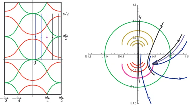
[image:18.612.142.457.85.262.2]1.5 1.0 0.5 0.5 1.0 1.5
Figure 4: On the left figure analytic continuation paths are shown on the z-torus. On the right figure blue curves represent the lines x+(z) corresponding to the torus variablezgoing upward from the real line to the line with Im(z) =ω2/i and they have |Re(z)| ≤ ω1
4 . Black curves x+(z) correspond to z going upward and have |Re(z)| ≥ ω1
4 . Any black or blue curve intersects the lowest curve inside the circle. Paths sufficiently close to the lines |Re(z)| ≤ ω1
4 do not intersect any cut except the lowest curve and, therefore, they are used for analytic continuation.
regionsR1,0, R2,0,R1,1 andR2,1, and to prove the crossing equations for the regions
R0,0 ↔ R2,0 andR0,1 ↔ R2,1. Then, unitarity together with crossing equations allow
one to continue analytically the dressing factor to any region Rm,n. However, since the regionR1,1 contains the real momentum line of the mirror theory, we decided to
analytically continue the dressing phase to the region R3,1 without appealing to the
crossing equations, and to check them for these regionsR1,1 ↔ R3,1.
Region R1,0: {z1, z2} ∈ R1,0 =⇒ |x1+|<1, |x−1|>1 ; |x±2|>1
First we discuss the analytic continuation from the particle regionR0,0 to the region
R1,0 where |x+1|<1, |x−1|>1 ; |x±2|>1.
We want to understand which curves x(±n) are crossed when the point z1 moves
upward along a vertical line in the z-torus and enters the region R1,0, see Figure 4.
In this region we need to analyze the functions χ(x+1, x±
2) only . Since the integral
representation for χ is well-defined for |x+1| > rcr, the dressing phase is obviously a
holomorphic function in the vicinity of the curve |x+1| = 1, and it can be evaluated there by using (3.23). The dressing phase cannot be however holomorphic everywhere inR1,0, because the curves x±(n)have images in this region, and the function Ψ(x+1, x±2)
is discontinuous across the curves. The images of the curves x(±n) inR1,0 are the cuts
A simple analysis reveals that no cuts are met in the intersection of the region
|x+1|<1, |x−1|>1 with the region Im(x±1)<0, see also Figure 4. Thus, the dressing
phase is a holomorphic function in this intersection. The region Im(x±
1) < 0 also
contains the line corresponding to the real momentum of a mirror particle. It was considered as a natural candidate for the region of the mirror theory in [9] because it contains one of the 2Q−1 solutions to the Q-particle bound state equations and
is in one-to-one correspondence with the u-plane. A choice of the mirror region is not however unique, and in particular the Q-particle bound state solution used in [45]5 does not fall in the region Im(x±1) < 0. For this reason we are reluctant
to refer to the region Im(x±
1) < 0 as a mirror one. Still, the region Im(x±1) < 0
seems to be special because the dressing factor is analytic there. This follows from the consideration above, and from the fact that the dressing factor for fundamental particles is obviously analytic in the region R2,0 due to the crossing equation. We
will return to the issue of non-uniqueness of bound state solutions in our conclusions. Dragging z1 upwards, we observe that the first curve the point x+(z1) reaches
is x(1)+ =x+(z1), |x−(z1)|= 1 that is the lower boundary of the anti-particle region
|x+1|<1,|x−1|<1 and that is the image of the curve closest to the circle in the lower x+-half-plane.
We conclude, therefore, that in the case of fundamental particles the analytic branch of the functions χ(x±1, x±2) in the region R1,0 can be defined as
R1,0 : χ(x+1, x±2) = Φ(x+1, x±2)−Ψ(x+1, x±2), (4.1)
χ(x−1, x±2) = Φ(x−1, x±2), (4.2)
where Ψ is given by (3.6). Let us also mention that the region R−3,0 obtained by
shifting the point z1 downward also has |x+1| < 1, |x−1| > 1. The dressing phase,
however, differs there from (4.1) by the double crossing term (2.11).
Region R2,0: {z1, z2} ∈ R2,0 =⇒ |x1+|<1, |x−1|<1 ; |x±2|>1
Dragging the pointz1 further upward into the anti-particle region|x±1|<1, we must
inevitablycross the curve x(1)+ , the latter maps to the one-cycle|x−
1|= 1 of thez-torus.
Then the formula (3.23) for χ(x+1, x2) should be modified because, as was discussed
in the previous section, one pole of the first ψ-function in (3.6) moves outside the circle and another one moves inside. Therefore, once the point z1 crosses the lower
boundary of the anti-particle region|x±1|<1, we should add to Ψ the following term 1
i log
w(x+1)−x±
2 1
w(x+1) −x
±
2
, (4.3)
5Strictly speaking in [45] the real momentum line of the mirror theory was obtained by shifting
the realz-axis byω1
!1
4
!1
4
!1
2
!1
2
¡!1
2
¡!1
2 ¡
!1
4
¡!1
4
!2
2
!2
2
!2 !2
0 0
-2 -1 1 2
-2
-1
[image:20.612.130.470.83.281.2]1 2
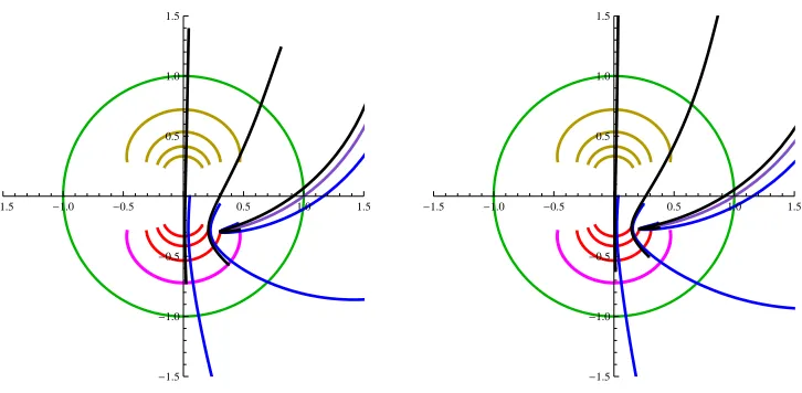
Figure 5: Blue and black curves on the right figure represent the curves x−(z) corresponding to the curves x+(z) in Figure 4. No black curve in-tersects the cuts inside the circle, and the blue curves close enough to Re(z) = ω1
4 do not intersect the cuts either.
where we have taken into account the formula (3.13) for the jump discontinuity of the Ψ-function. Here w(x+1) solves the equation x+1 + x1+
1 −w −
1
w =
2i g and satisfies |w(x+1)|<1. Since |x−
1|<1 oncez1 crosses the boundary, we conclude that
w(x+1) = x−
1. Thus, we get the following expressions for the functions χ with the
first particle being in the anti-particle regionR2,0
R2,0 : χ(x+1, x±2) = Φ(x1+, x±2)−Ψ(x+1, x±2) +
1 i log
1
x−
1 −x
±
2
x−
1 −x±2
, (4.4)
χ(x−
1, x±2) = Φ(x−1, x±2)−Ψ(x−1, x±2), (4.5)
where|x+1|<1, |x−
1|<1 and|x±2|>1, and the functions Φ and Ψ are given by (3.1)
and (3.6) for all values ofx±
1 from the region. Let us stress that in the z1-plane the
anti-particle region is obtained from the particle region containing the realz-axis by shifting it by ω2 upward.
These formulae define a certain analytic branch of the functions χ(x±1, x±2) in
R2,0 and, as will be discussed in the next subsection, they are sufficient to prove the
crossing equation for z1, z2 being in the particle region. It is worth stressing that
even though the functions χ are not analytic in the region R2,0 because of the cuts
located in the intersection of the anti-particle region with the regions Im(x±)<0 and
Im(x±)>0, as is evident from Figures 4 and 5, the dressing factor itself is analytic
inR2,0 because it is related to the dressing factor inR0,0 by the crossing equation.
derived by deforming the integration contour in (3.1) and (3.6). In other words, the curve |x−(z)|= 1 is not a cut of the dressing phase6 but rather the boundary of
va-lidity of the integral representation forχ. Crossing this curve enforces a modification of the integral representation, as described above.
In our treatment above we have chosen a path for analytic continuation of the dressing phase by starting with the variablez1 from the particle region and dragging
it upward from the real axes. Analogously, we could consider a path of different orientation, i.e. the one which is obtained by shifting z1 downward from the real
axis. The interested reader may consult the appendix, where the results of this analytic continuation are sketched. Now we find the analytic continuation for the dressing phase in the regions Rk,1, k = 2,3,. This is relevant for proving that the
dressing phase of the mirror theory also satisfies the same crossing equations.
Region R1,1: {z1, z2} ∈ R1,1 =⇒ |x+1|<1, |x−1|>1 ; |x+2|<1, |x−2|>1
Consider the case where the particles are in the regionR1,1 with |x+k| <1,|x−k|>1 obtained from the regionR0,0 by moving both pointsz1 andz2 upward. If the second
particle is in the region |x±
2|>1 the functions χare given by (4.1) and (4.2). If the
point z2 is shifted upward, then we should add the extra contributions coming from
Φ and Ψ functions, and we derive the following expressions for the functions χ
R1,1 : χ(x+1, x+2) = Φ(x+1, x2+) + Ψ(x+2, x+1)−Ψ(x+1, x+2)
+ilog
Γ1 + i
2g x + 1 +x1+
1 −x
+ 2 − x1+
2
Γ1− i
2g x + 1 +x1+
1 −x
+ 2 − x1+
2 ,
χ(x+1, x−
2) = Φ(x+1, x−2)−Ψ(x+1, x−2),
χ(x−
1, x+2) = Φ(x−1, x2+) + Ψ(x+2, x−1),
χ(x−1, x−2) = Φ(x−1, x−2), (4.6)
where the last term in the formula forχ(x+1, x+2) comes from the analytic continuation of Ψ(x+1, x+2) in z2 shifted upward.
Region R2,1: {z1, z2} ∈ R2,1 =⇒ |x+1|<1, |x−1|<1 ; |x+2|<1, |x−2|>1
Shifting z1 further upward into the anti-particle region, we get
R2,1 : χ(x+1, x+2) = Φ(x+1, x2+) + Ψ(x+2, x+1)−Ψ(x+1, x+2) +
1 i log
1
x−
1 −x
+ 2
x−1 −x+2
+ilog
Γ1 + i
2g x + 1 + x1+
1 −
x+2 − 1
x+2
Γ1− i
2g x + 1 +x1+
1 −x
+ 2 − x1+
2 ,
χ(x+1, x−
2) = Φ(x+1, x−2)−Ψ(x+1, x−2) +
1 i log
1
x−
1 − x−
2
x−1 −x−2 , χ(x−1, x+2) = Φ(x−1, x+2)−Ψ(x−1, x+2) + Ψ(x+2, x−1)
+ilog
Γ1 + i
2g x−1 + x1−
1 −
x+2 − 1
x+2
Γ1− i
2g x−1 +x1−
1 −x
+ 2 −x1+
2 ,
χ(x−
1, x−2) = Φ(x−1, x−2)−Ψ(x−1, x−2). (4.7)
Region R3,1: {z1, z2} ∈ R3,1 =⇒ |x+1|>1, |x−1|<1 ; |x+2|<1, |x−2|>1
Dragging the point z1 further upward into the region |x−1| < 1, |x+1| > 1, we cross
the curve x(1)− that is mapped to the curve |x+1| = 1 on the z-torus, the latter being the upper boundary of the anti-particle region.
Thenx+1 goes outside the unit circle and we need to drop Ψ function from (4.4), and x−
1 crosses x (1)
− , and produces an extra contribution to (4.7) because one pole of
the secondψ-function in (3.6) moves outside the circle and another one moves inside. The result of the analytic continuation is then given by
R3,1 : χ(x+1, x+2) = Φ(x+1, x+2) + Ψ(x+2, x+1) +
1 i log
1
x−
1 −x
+ 2
x−1 −x+2 ,
χ(x+1, x−2) = Φ(x+1, x−2) +
1 i log
1
x−
1 −x
−
2
x−
1 −x−2
,
χ(x−1, x+2) = Φ(x−1, x+2)−Ψ(x−1, x+2) + Ψ(x+2, x−1) + 1 i log
1
x+1 −x
+ 2
x+ 1 −x+2
+ilog
Γ1 + i
2g x−1 + x1−
1 −x
+ 2 −x1+
2
Γ1− i
2g x−1 +x1−
1 −x
+ 2 −x1+2
,
χ(x−
1, x−2) = Φ(x−1, x2−)−Ψ(x−1, x−2) +
1 i log
1
x+1 −x
−
2
x+1 −x−
2
. (4.8)
4.2 The crossing equations for fundamental particles
Having obtained the dressing phase as an analytic function with cuts on the product of two infinite strips −ω1
2 ≤ Im(z) ≤
ω1
2, we can now evaluate the left hand side of
the crossing equation
∆θ ≡θ(z1, z2) +θ(z1+ω2, z2).
In terms of the χ-functions ∆θ takes the form ∆θ =χ(x+1, x+2)−χ(x+1, x−
2)−χ(x−1, x2+) +χ(x−1, x−2)
+χ(1/x+1, x+2)−χ(1/x+1, x−
2)−χ(1/x−1, x+2) +χ(1/x−1, x−2),
(4.9)
Considered as the function on two z-planes, the crossing equation must hold for any choice of the pair {z1, z2}. In what follows we will restrict ourselves to checking the
crossing equation for two different cases, namely for {z1, z2} ∈ R0,0 and {z1, z2} ∈
R1,1. We recall that these cases correspond to both z1 and z2 being in the particle
region or in the region relevant for the mirror theory, respectively.
We start with the case {z1, z2} ∈ R0,0 ⇒ |x±1| >1 ; |x±2|>1. Then, |1/x±|<1
and, therefore, the arguments of the χ-functions occurring in the second line of eq.(4.9) are in the region R2,0. Thus, evaluating the second line in eq.(4.9), we have
to use the formulae (4.4) and (4.5) with the substitution in the latter x±1 → 1/x±1.
Taking into account the identity (3.4), one finds that the contribution of Φ-functions in ∆θ cancels out and one gets
∆θ = Ψ( 1 x−
1
, x+2)−Ψ( 1 x+1 , x
+ 2) + Ψ(
1 x+1 , x
−
2)−Ψ(
1 x−
1
, x−2)
+ 1 i log
x−1 −x+2
1
x−
1 −x
+ 2
1
x−
1 − x−
2
x−
1 −x−2
. (4.10)
The Ψ-function satisfies a number of important identities which are listed in appendix 8.2. In particular, by using the formula (8.4) valid in the region|x±1|>1 and|x2|>1,
we get
Ψ( 1 x−1 , x
+
2)−Ψ(
1 x+1 , x
+ 2) + Ψ(
1 x+1 , x
−
2)−Ψ(
1 x−1 , x
−
2) =
1 i log
(1−x−1
1x+2 )(1−
1
x+1x+2) (1− x−1
1x−2 )(1−
1
x+1x−
2) .
Finally,
∆θ = 1 i log
(1− 1
x−
1x+2 )(1−
1
x+1x+2) (1− x−1
1x−2 )(1−
1
x+1x−
2 ) + 1
i log
x−1 −x+2 1
x−
1 −x
+ 2
1
x−
1 −x
−
2
x−
1 −x−2
= 1 i log
hx−
2
x+2 h(x1, x2) i
,
which is the correct crossing equation for the dressing phase of fundamental particles. Now we would like to verify the crossing equations for the case{z1, z2} ∈ R1,1 ⇒
|x+1| < 1, |x−
the arguments of the χ-functions in the second line of eq.(4.9) are in the region
R3,1. Thus, evaluating the second line in eq.(4.9), we have to use the formulae (4.6)
and (4.8) with the substitution in the latter x±
1 → 1/x±1. With the account of the
identities (3.4) and (3.15), we get
∆θ = Ψ( 1 x−
1
, x+ 2)−Ψ(
1 x+1 , x
+ 2) + Ψ(
1 x+1 , x
−
2)−Ψ(
1 x−
1
, x−
2)
+1 i log
x−1 −x+2
1
x−
1 −x
+ 2
1
x−
1 −x
−
2
x−
1 −x−2
+1 i log
x+1 −x−2
1
x+1 −x
−
2 1
x+1 −x
+ 2
x+1 −x+2 (4.11)
+1 i log
Γ1 + i
2g x−1 +x1−
1 −x
+ 2 − x1+
2
Γ1− i
2g x−1 +x1−
1 −x
+ 2 − x1+
2
Γ1− i
2g x + 1 + x1+
1 −x
+ 2 − x1+
2
Γ1 + i
2g x + 1 + x1+
1 −x
+ 2 − x1+
2 .
First, the ratio of the Γ-functions is simplified to
1 i log
Γ1 + i
2g x−1 +x1−
1 − x+
2 − x1+ 2
Γ1− i
2g x−1 +x1−
1 −
x+2 − 1
x+2
Γ1− i
2g x + 1 + x1+
1 − x+
2 − x1+ 2
Γ1 + i
2g x + 1 +x1+
1 −
x+2 − 1
x+2
(4.12) = 1 i log g2 4(x −
1 −x+2)(x+1 −x+2)(1−
1
x−1x+2 )(1− 1 x+1x+2 ). Second, by using the identities (8.5) and (8.10), one obtaines
Ψ( 1 x+
1
, x−2)−Ψ( 1 x−
1
, x−2) = 1 i log
x−2 (x−1
1x−2 −1)(x
+
1 −x−2)
, (4.13)
Ψ( 1 x−
1
, x+2)−Ψ( 1 x+
1
, x+2) = 1 i log
4 g2
x+1 x+ 2
1
(x+2 −x−1)(x+1 −x1+ 2 )
. (4.14)
Substituting these results in eq.(4.11), we again recover the crossing equation (2.8). This verification of the crossing equation forR1,1 confirms correctness of our analytic
continuation of the dressing phase into this region.
5. Bound state dressing factor of string theory
In this section we discuss the analytic continuation of the dressing phaseθQM(z
1, z2)
for the scattering matrix ofQ-particle andM-particle bound states. Further, we use this continuation to prove the general crossing equations (2.14).
5.1 Analytic continuation of the bound state dressing phase
As was reviewed in section 2, in the particle region |x±| > 1 and in terms of the
-1.5 -1.0 -0.5 0.5 1.0 1.5
-1.5 -1.0 -0.5
0.5 1.0 1.5
-1.5 -1.0 -0.5 0.5 1.0 1.5
-1.5 -1.0 -0.5
[image:25.612.118.481.80.258.2]0.5 1.0 1.5
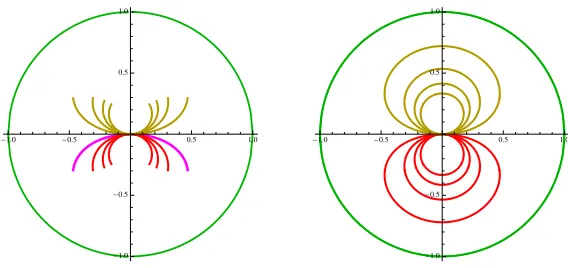
Figure 6: On the left picture blue curves represent x+(z) corresponding to z going upward from the real line of the z-torus of a two-particle bound state to the line with Im(z) = ω2/i and have |Re(z)| ≤ ω41. Black curves x+(z) correspond to z going upward and they have |Re(z)| ≥ ω1
4 . Any blue curve intersects the second lower curve in the circle. On the right picture a three-particle bound state is considered, and any blue curve intersects the third lower curve. Curves x−(z) are shown in Figure 10.
is incompatible with the crossing equations (2.14), which were derived from the ones for fundamental particles by using the fusion procedure.
In this subsection we identify the analytic continuation of the dressing phaseθQM which leads to eqs. (2.14). We assume here that the first and the second particles are Q- and M-particle bound states, respectively, and that their kinematic parameters x±1 and x±2 obey the constraints (2.13).
Region R1,0: {z1, z2} ∈ R1,0 =⇒ |x1+|<1, |x−1|>1 ; |x±2|>1
Again, we begin with defining the analytic continuation from the particle regionR0,0
to the regionR1,0 whose kinematic description is given above.
We first need to determine which curves x(±n) are crossed when the pointz1moves
upward along a vertical line in the z-torus and enters the region R1,0, see Figure 6.
Recall that in the case of fundamental particles, the point z1 in the intersection of
the region R1,0 with the region Im(x±) < 0 does not cross on its way the image
of any curve x(±n), until it reaches the curve |x−
1| = 1 that is the upper boundary
of R1,0 and an image of x(1)+ . As a result, the dressing phase θ11 ≡ θ appears to
be a meromorphic function in this intersection. In the Q-particle case the upper boundary of R1,0 is an image of the curve x(+Q), as is evident from eq. (3.11), and
there are images of the first Q−1 curves x(+n) in the intersection of R1,0 with the
-1.0 -0.5 0.5 1.0
-1.0
-0.5
0.5 1.0
-1.0 -0.5 0.5 1.0
-1.0
-0.5
[image:26.612.155.439.81.215.2]0.5 1.0
Figure 7: On the left picture the curves ˇx(±n) = 1/x(u±2gin) with |u| ≥2 for g = 3 and n = 1,2,3,4. The endpoints of the curves correspond to u = ±2. The curves closest to the real line correspond to n = 1. On the right picture the curves 1/x(u±2gin) with |u|<∞ are shown.
which therefore are not allowed to be crossed, then the analytic continuation of the dressing phase would obviously be the same as for fundamental particles. It turns out, however, that the crossing equations force us to analytically continue across the curves x(+n), and, therefore, the cuts in the z-plane should be chosen complementary
to the images of x(+n).
A convenient and natural choice of the cuts in thex- andz-planes is provided by eq.(3.10). This equation suggests to identify the cuts with the curves ˇx(+n) = x(u+12i
gn)
, n = 1, . . . , Q−1, but where the parameter u takes values in the region|u| ≥2. In the x-plane all these curves go through the origin x= 0 corresponding to u=±∞, see Figure 7. In the z-plane the images of the curves are in the intersection of the region R1,0 with the region Im(x±) < 0, and the origin x = 0 corresponds to the
pointsz =−ω1
2 +
ω2
2 andz =
ω1
2 +
ω2
2 that are one and the same point on thez-torus.
Obviously, the union of the curves x(+n) and ˇx (n)
+ is a closed curve in the x-plane,
and for n = 1, . . . , Q−1 its image in the region R1,0 is a one-cycle and divides the
z-torus in two parts. Let us denote the corresponding curve in the z-torus as X+(n). Thus, the region R1,0 is divided by these curves into Q smaller regions, see Figure
8. We denote the region bounded by the curves X+(n−1) and X (n)
+ as Rn1,0, where
n= 1, . . . , Q. The curve X+(0) is the lower boundary of the regionR1,0 with|x+1|= 1,
while the curve X+(Q) = x (Q)
+ is the upper boundary of R1,0 with|x−1|= 1.
Thus, to reach the regionRn
1,0, one should analytically continue through the first
n−1 curves x(+n). Therefore, in contradistinction to the case of fundamental particles, one gets n−1 extra contributions. As we will see, when properly combined, these extra contributions lead to the correct crossing equation.
!1 4 !1 4
!1 2 !1 2
¡!1 2
¡!1 2 ¡
!1 4
¡!1 4
!2 2 !2 2
!2 !2
0
!1 4 !1 4
!1 2 !1 2
¡!1 2
¡!1 2 ¡
!1 4
¡!1 4
!2 2 !2 2
[image:27.612.168.431.82.244.2]!2 !2
Figure 8: Division of R1 into smaller regions by curves χ(+n) is shown for two-particle (the left figure) and three-particle (the right figure) bound states. The cuts ˇx(+n) of the dressing phase are drawn in purple. In the two-particle case, the curve χ(1)+ coincides with the real line of the mirror theory.
the region R1,0 are the cuts of the dressing phase on the z-torus, see Figure 9, and
the analytic continuation of the functionsχ(x±
1, x±2) in the region Rn1,0 is given by
Rn1,0 : χ(x+1, x±2) = Φ(x1+, x±2)−Ψ(x+1, x±2)−
1 i log
n−1
Y
j=1
wj−(x+1)−x±2 1
w− j(x
+ 1) −
x±
2
, (5.1)
χ(x−
1, x±2) = Φ(x−1, x±2),
where n = 1, . . . , Q. Here we have introduced the functions w±
j (x) defined as the solutions to the following equations
x+ 1 x −w
−
j − 1 wj−
= 2i
g j , w
+
j + 1 wj+
−x− 1 x =
2i
gj , |w
±
j |<1. (5.2)
General solutions to these equations can be given in terms of the function x(u) as follows
w−
j (x
+
1) = wQ+−j(x−1) =
1
x(u1+ gi(Q−2j))
, (5.3)
where we introduce the u1-plane variable
u1 =x+1 +
1 x+1 −
i
gQ=x
−
1 +
1 x−
1
+ i
gQ . (5.4)
-1.0 -0.5 0.5 1.0
-1.0
-0.5
0.5 1.0
-1.0 -0.5 0.5 1.0
-1.0
-0.5
[image:28.612.157.438.81.213.2]0.5 1.0
Figure 9: On the left and right pictures the x-plane the cuts of two- and three-particle bound state dressing factors in the regionR1,0are shown. The yellow curves are x(+Q) with Q= 2,3, and they are not cuts of the dressing factors.
Q+ 1, . . .∞, and x(−n), n= 1, . . .∞ are given by the following line segments
ˇx(+n) : u1 =u−
i
g(Q−2n), |u| ≥2, n= 1, . . . , Q−1, (5.5) x(+n) : u1 =u−
i
g(Q−2n), |u| ≤2, n=Q+ 1, . . . ,∞, (5.6) x(−n) : u1 =u+
i
g(Q−2n), |u| ≤2, n= 1, . . . ,∞. (5.7)
As was already mentioned above, the images of the curves ˇx(+n),n= 1, . . . , Q−1, and x(+n), n =Q+ 1, . . .∞, and x
(n)
− , n = 1, . . .∞ in the region R1,0 are the cuts of
the dressing phase on the z-torus, see Figures 8 and 9 . We also point out that if Q= 2m is even then the cut with n=m falls on the real line of the mirror theory! Indeed, from eq.(5.5) we see that for ˇx(+m) the parameteru1 coincides with the real u
obeying |u| ≥2. We also see that for Q = 2m the curve X+(m) is the real line of the mirror theory.
Region R2,0: {z1, z2} ∈ R2,0 =⇒ |x1+|<1, |x−1|<1 ; |x±2|>1
Moving the pointz1 from the regionRQ1,0 further upward into the anti-particle region
R2,0 with |x±1| < 1, we cross the curve x (Q)
+ that is mapped to the curve |x−1| = 1
-2 -1 1 2
-2 -1
1 2
-2 -1 1 2
-2 -1
[image:29.612.116.482.77.260.2]1 2
Figure 10: Blue and black curves represent x−(z) corresponding to the
curvesx+(z) in Figure 6. No black curve intersects the cuts inside the circle but they all touch the upper cut. The blue curves close enough to Re(z) = ω1
4 do not intersect the cuts either.
with the first particle being in the region R2,0
R2,0 : χ(x+1, x±2) = Φ(x1+, x±2)−Ψ(x+1, x±2)−
1 i log
Q−1
Y
j=1
w−
j (x
+ 1)−x±2 1
w− j(x
+ 1)−x
±
2
(5.8)
+ 1 i log
1
x−
1 −x
±
2
x−
1 −x±2
,
χ(x−
1, x±2) = Φ(x−1, x±2)−Ψ(x−1, x±2).
It is worth noting that the cuts of the functions w−
n(x+1) on thez-torus coincide with
the images of the curve x(+n) , and, therefore, they are already included in the cut
structure of the χ-functions. As we will show in the next subsection, the dressing factor satisfies the crossing equation, and is an analytic function inR2,0.
Region R1,1: {z1, z2} ∈ R1,1 =⇒ |x+1|<1, |x−1|>1 ; |x+2|<1, |x−2|>1
Finding the analytic continuation to the region R1,1 basically follows the ones in
the previous section, and forR1,0. Since the second particle is an M-particle bound
state, the region |x+2| <1, |x−2| >1 should be divided into M smaller regions, and, as a consequence, R1,1 should be understood as a union ofQ×M regions which we