Compositional reasoning for weighted Markov decision processes

(1)

Contents lists available atSciVerse ScienceDirect

Science of Computer Programming

journal homepage:www.elsevier.com/locate/scico

Compositional reasoning for weighted Markov

decision processes

Yuxin Deng

a,∗

, Matthew Hennessy

b

a_{Shanghai Jiao Tong University, China}

b_{Trinity College Dublin, Ireland}

h i g h l i g h t s

• We develop compositional methods for reasoning about weighted Markov decision processes (MDPs). • A coinductive simulation-based behavioural preorder is proposed for weighted MDPs.

• The preorder is preserved by structural operators for constructing weighted MDPs from components.

• For finitary convergent processes, the preorder can be characterised by a probabilistic logic and a novel form of testing.

a r t i c l e i n f o

Article history:

Received 11 November 2011

Received in revised form 18 December 2012 Accepted 21 February 2013

Available online xxxx

Keywords:

Markov decision processes Simulation

Testing preorder Modal logic Compositionality

a b s t r a c t

Weighted Markov decision processes (MDPs) have long been used to model quantitative aspects of systems in the presence of uncertainty. However, much of the literature on such MDPs takes a monolithic approach, by modelling a system as a particular MDP; properties of the system are then inferred by analysis of that particular MDP. In contrast in this paper we develop compositional methods for reasoning about weighted MDPs, as a possible basis for compositional reasoning about their quantitative behaviour. In particular we approach these systems from a process algebraic point of view. For these we define a coinductive simulation-based behavioural preorder which is compositional in the sense that it is preserved by structural operators for constructing weighted MDPs from components.

For finitary convergent processes, which are finite-state and finitely branching systems without divergence, we provide two characterisations of the behavioural preorder. The first uses a novel quantitative probabilistic logic, while the second is in terms of a novel form of testing, in which benefits are accrued during the execution of tests.

1. Introduction

Markov decision processes (MDPs) have long been used to model quantitative aspects of systems in the presence of uncertainty [33,34,5]. A comprehensive account of analysis techniques may be found in [33], while [34] provides a good account ofmodel-checking.

We are particularly interested in a sub-class of MDPs, in which actions have associated with them an explicitcostor

reward, which we refer to asweighted MDPs. However much of the literature on this class of MDPs takes a monolithic view of systems; essentially a system is modelled using a particular (weighted) MDP, and properties of the system are then inferred by analysis of that MDP. The literature on the related model of weighted automata [11] is similar in nature. In this paper, instead, we would like to develop compositional methods for reasoning about quantitative behaviour of these

∗_{Corresponding author.}

(2)

s0

sd

up₃ down1

t0

td

up2

down4

u0

τ

0

τ

1

up₁

τ

2

down1

[image:2.544.58.471.54.366.2]

up₁

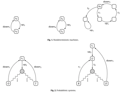
Fig. 1.Nondeterministic machines.

s1

O T

up₂

1 4

3 4

down3

down1

t1

U

R D

up₂

τ

0

3 4

1 4

τ

1

down₁

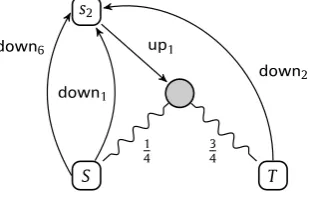
Fig. 2.Probabilistic systems.

kinds of Markov decision processes. This involves devising a method for comparing their behaviour which is susceptible to compositional analysis; the behaviour of a composite system should be determined by that of its components.

Our starting point is the idea of one system being able tosimulateanother. For example consider the three systems in Fig. 1. The first, a two-state machine, continually performs anupaction, which accrues a benefit of 3 units, followed by adownaction, which accrues a benefit of 1. The second machine performs the same actions but with benefits 2 and 4 respectively. In some senset0is an improvement ons0; intuitivelyt0can simulate the behaviour ofs0but in so doing accrue

more benefits; this is true even if one of its actionsupis less beneficial than the corresponding action ofs0. The same is true

for the machineu0; it can also simulate the behaviour ofs0, with more benefit, although in this case some internal weighted

actions, denoted by

τ

, participate in the simulation and add to the accumulation of benefits. In our terminology we will write

s0

⊑

simt0

,

s0

⊑

simu0

.

However we will havet0

̸⊑

simu0because althoughu0can simulate the behaviour oft0it accumulates

less benefit.

Similar informal reasoning can also be applied to probabilistic systems. Consider the systems inFig. 2. Here we have two kinds of nodes; the first as inFig. 1representing states of the systems, and the second representing probability distributions. For example the first system, from states1, can perform theupaction with benefit 2 and a quarter of the time it ends up in

a state in whichdowncan be performed with benefit only 1. But for the remaining three-quarters it ends up in a state in whichdowncan be performed for the larger benefit 3. The circular darkened node represents a distribution of states, with its outgoing edges describing the associated probabilities. Again intuitively we can see thats1is an improvement ons0because

it can simulates0and on average accrue slightly more benefits; in our theory we will haves0

⊑

sims1.

The mixture of probabilistic behaviour and internal actions introduces complications. Consider the systemt1inFig. 2

which after performing anupaction probabilistically decides internally whether to perform adownaction for benefit 1, or branch back to make another probabilistic choice. However each time it reverts back it accumulates a non-zero benefit via the internal weighted action

τ

1, albeit with diminishing probability. Nevertheless it will turn out that for our definition of

simulations0

⊑

simt1and indeeds1

⊑

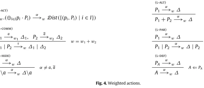
simt1.

Systems exhibiting both probabilistic and nondeterministic behaviour require more complicated analysis. Consider the system inFig. 3. After performing the actionupit finds itself either in a state in which the actiondownwill accrue the benefit 2, or 25% of the time there will be a nondeterministic choice between it accruing either 1 or 6. In the literature there are numerous mechanisms, such as policies, schedulers, adversaries, etc. [33,35,34] for resolving such choices. Here one can see if this choice systematically leads to the lower benefit 1 thens2will not simulates0as it does not accrue sufficient benefits.

(3)

s2

S T

up₁

1 4

3 4

down2

down1

[image:3.544.194.349.65.170.2]

down₆

Fig. 3.Nondeterministic and probabilistic systems.

The main contribution of the paper is a coinductively defined behavioural preorder

⊑

_simbetween weighted MDPs based on simulations which validate the examples discussed informally above. We confine our attention to the optimistic approach to the resolution of nondeterministic choices, although as future work we hope to investigate the pessimistic approach. We also show that this preorder is compositional in the sense that it is preserved by structural operators for constructing (weighted) MDPs from components. The main operator is one for composing two such MDPs in parallel. InP

|

Q the two MPDsPandQremain independent, execute in parallel and may communicate by synchronising on complementary actions; these internal synchronisations accrue the combined benefits of the associated complementary actions.

We also provide two independent characterisations of the behavioural preorder

⊑

_simfor a particular class of well-behaved systems. These are weighted MDPs which are finite-state and finitely branching systems without divergence, which we refer to as finitary convergent weighted MDPs. The first characterisation is in terms of aquantitative probabilistic logicL. In addition to the standard logical connectives such as conjunction and a maximal fixed point operator, this contains a novel quantitativepossibilitymodality

⟨

α

⟩

_w

(φ

₁p

⊕

φ

2

)

, wherepis some probability between 0 and 1. Intuitively this is satisfied

by an MDP which can accrue at least the benefit

w

by performing the action

α

, and subsequently satisfy the probabilistic assertion

φ

1p

⊕

φ

2. It turns out that the simulation preorder is completely determined by the logicL. Further evidence of

the compatibility between the logic and the simulation relation is the fact that every systemPhas acharacteristic formula

φ(

P

)

in the logic which captures its behaviour; informally systemQcan simulatePif and only if it satisfies the characteristic formula

φ(

P

)

.

Our second characterisation is in terms of a novel form of testing calledbenefitstesting. Intuitively a systemPcan be tested by running it in parallel with another testing systemT, and seeing the possible accrued benefits. In the presence of nondeterminism the execution of the combined system

(

T

|

P

)

will result in a non-empty set of benefits,Benefits

(

T

|

P

)

. Then systemsPandQcan be compared by comparing the associated benefit setsBenefits

(

T

|

P

)

andBenefits

(

T

|

Q

)

where

Tranges over some collection of possible tests. We show that the simulation preorder

⊑

_simis also determined in this manner by a suitable collection of testsT.

The rest of this paper is organised as follows. Section2is devoted to an exposition of our model, which we callweighted Markov Decision Processes,wMDPs. These correspond to the diagrams we have been using informally in this introduction. The actions in a wMPD take the forms

−→

α _w ∆, where

α

is the label of the action,

w

its weight, or benefit, and∆a probability distribution which determines the next state. Following [35,36,14], we make extensive use of the generalisation of this next-step relation to actions from distributions to distributions,∆

−→

α _w Θ. Furthermore we are interested in

weaktheories, in which internal activity is not directly observable. So we generalise these actions to weak actions, of the forms

=⇒

α _w ∆and∆

=⇒

α _w Θrespectively, actions in which occurrences of internal actions, denoted by

τ

, may occur an arbitrary number of times both before and after

α

. As have already been pointed out by many authors, [27,14], in a probabilistic setting we need to allow a potentially infinite number of internal actions to occur,in the limit; we follow the formalisation of this idea suggested in [14]. One particularly significant property, which underlies much of our technical results, is that the set of weak derivatives from a given state, although in general uncountable, in a finite-state wMDP can be generated as the convex-closure of a finite number of derivatives. This is explained in Section2.4. The proof is very complex, relying on notions such as static policies and payoffs [14]. Consequently, again the details are relegated to an appendix.

Then, still in Section2, we turn our attention to a sub-class of wMDPs, calledbounded wMDPs. In an arbitrary wMDP if

∆

=⇒

τ _w Θthen

w

may in general be infinite because of an indefinite accumulation of weights during an infinite internal computation. In bounded wMDPs we are guaranteed that such

w

s will always be a finite real number. Such wMDPs are the main focus of the paper, and their properties are studied in Section2.5.

(4)

by a very simple modal logic, again if we restrict attention to bounded wMDPs. This logic is quantitative in the sense that satisfying formulae depends to some extent on the benefits which a process can accrue. The logical characterisation in turn depends on the approximation result from Section3.2.

In Section4we offer another justification for our simulation based on testing [31]. Because of the presence of weights or benefits in wMDPs we are able to use a novel form of (may) testing in which benefits are accrued as tests are applied to processes; then processes can be compared in terms of their ability to accumulate benefits. In Section4.1this idea,benefits testing, is explained in detail and we also show that it is preserved by the simulation preorder. More interesting is the result, for bounded wMDPs, that the preorder is completely determined by these tests. This proof requires a digression, in Section4.2, into a more standard testing framework. Here we extend the ideas on [36,15] by developing a version of multi-success testing suitable for wMDPs. In a non-trivial theorem we show that in bounded wMDPs both testing preorders, benefit-based and multi-success, coincide. The interest in multi-success testing is that we can mimic the results in [14] to show that this form of testing can be captured by the modal logic of the previous section. Since we already know that the modal logic determines the simulation preorder we have therefore also established the soundness and completeness of benefits testing for the simulation preorder.

Section4ends with a short discussion of another natural form of testing,expected benefits testing, in which the average weight of each path of a computation leading to a success is associated with a test. By means of a simple example we show that the simulation preorder is not sound for this form of testing.

2. Weighted Markov decision processes

In this section we give a precise account of our version of MDPs and develop their technical properties which will be needed in the remainder of the paper. The formal definition of our weighted MDPs is given in Section2.1where we also define a process calculus, based on CCS, [29], for describing them. In the following Section2.2we show how to generalise the relationss

−→

µ _w Θfound in weighted MDPs, to relations over (sub-)distributions,∆

−→

α _w Θ; we also outline some elementary properties of this construction. The approach taken is very similar to that in [14] but a proper account of the weights of actions needs to be given.

In the following Section2.3we give our definition ofweak weighted arrows,∆

=⇒

τ _wΘin which, as previously stated, the internal activity may occur indefinitely, and probabilistically infinitely often. Again we follow closely the formal approach in [14], developing a weighted version of so-called hyper-derivations. We also give the rather large list of their properties which we require. However their proofs are relegated to an appendix, as they are somewhat technical.

This construction endows the set of (sub-)distributions of a weighted MDP with the structure of an Labelled Transition System (LTS) but in general the set of possible actions∆

=⇒

α _w Θ, even from a given distribution∆are uncountable. However if we put finitary restrictions on the MDP then it turns out that for a given∆the set of possible residualsΘcan be finitely generated; this is the topic of Section2.4.

Finally in Section2.5we see the particular class of MDPs on which the paper focuses. In general, because of the infinitary nature of weak moves∆

=⇒

τ _w Θthe actual weight associated with the move

w

may be infinite. We wish to rule out this possibility, and instead concentrate on a sub-class of MDPs, which we calledbounded, where this accumulation of infinite weight is not possible. In this section we give a natural condition which is sufficient to ensure boundedness.

2.1. Introduction

There is considerable variation in the literature in the formal definition of a (labelled) Markov decision process [34,33]. For the purpose of this paper we useDefinition 2.1to delineate our version of weighted MDPs. We first fix some notation. A (discrete) probabilitysubdistributionover a setSis a function∆

:

S

→ [

0

,

1

]

with



s∈S∆

(

s

)

≤

1; thesupportof such a ∆is

⌈

∆

⌉ := {

s

∈

S

|

∆

(

s

) >

0

}

, and itsmass

|

∆

|

is



s∈⌈∆⌉∆

(

s

)

. A subdistribution is a (total, or full)distributionif

|

∆

| =

1.

The point distributionsassigns probability 1 tosand 0 to all other elements ofS, so that

⌈

s

⌉ = {

s

}

. WithDsub

(

S

)

we denote the set of subdistributions overS, and withD

(

S

)

its subset of full distributions. For∆

,

Θ

∈

Dsub

(

S

)

we write∆

≤

Θiff

∆

(

s

)

≤

Θ

(

s

)

for alls

∈

S.

Let

{

∆k

|

k

∈

K

}

be a set of subdistributions, possibly infinite. Then



k∈K∆kis the real-valued function inS

→

Rdefined

by

(



k∈K∆k

)(

s

)

:=



k∈K∆k

(

s

)

. This is a partial operation on subdistributions because for some statesthe sum of∆k

(

s

)

might exceed 1. If the index set is finite, say

{

1

..

n

}

, we often write∆1

+ · · · +

∆n. Forpa real number from

[

0

,

1

]

we usep

·

∆

to denote the subdistribution given by

(

p

·

∆

)(

s

)

:=

p

·

∆

(

s

)

. Finally we use

ε

to denote the everywhere-zero subdistribution that thus has empty support. These operations on subdistributions do not readily adapt themselves to distributions; but if



k∈Kpk

=

1 for some collection ofpk

≥

0, and the∆kare distributions, then so is



k∈Kpk

·

∆k. In general when 0

≤

p

≤

1

we writexp

⊕

yforp

·

x

+

(

1

−

p

)

·

ywhere that makes sense, so that for example∆1p

⊕

∆2is always defined, and is full if ∆1and∆2are.

For∆

∈

Dsub

(

S

)

andf a function with domainS, we write Exp∆(f

)

, theexpected valueoff over∆

∈

Dsub

(

S

)

, for



s∈⌈∆⌉∆

(

s

)

·

f

(

s

)

. More generally supposef

:

S

k

→

_T_{. This is lifted to a function}_fĎ

:

_Dsub

(

_S

)

k

→

_Dsub

(

_T

)

_{by letting}

fĎ

(

∆1

, . . . ,

∆n

)(

t

)

=



t=f(s1,...,sk)∆1

(

s1

)

· · · · ·

∆k

(

sk

).

We will often abbreviate the lifted functionf

(5)

(l-act)

α

w

.(

⊕

i∈Ipi

·

Pi

)

−→

α wDist

(

{

(

pi

,

Pi

)

|

i

∈

I

}

)

(l-alt)

P1

−→

α w∆

P1

+

P2

α

−→

_w∆

(l-comm)

P1 a

−→

_w₁ ∆₁

,

P2 a

−→

_w₂ ∆₂

P1

|

P2

τ

−→

_w ∆₁

|

∆₂ w

=w1+w2

(l-par)

P1

α

−→

_w∆

P1

|

P2

α

−→

_w ∆

|

P2

(l-hide)

P

−→

α _w ∆

P

\

a

−→

α _w∆

\

a α

̸=a,a

(l-def)

PA

α

−→

_w∆

A

−→

α _w∆ [image:5.544.72.414.55.202.2]

A⇐PA

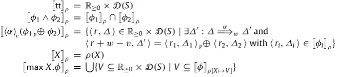
Fig. 4.Weighted actions.

Definition 2.1 (Weighted Markov Decision Process). Aweighted Markov decision processor wMDP is a 4-tuple

⟨

S

,

A

,

W

,

−→⟩

whereSis a set of states,Aa set of actions,Wa set of weights, and

−→ ⊆

S

×

A

×

W

×

D

(

S

)

. We normally writes

−→

α _w∆

to mean

(

s

, α, w,

∆

)

∈−→

.

In this paper we setWto be_R≥0, the set of non-negative real numbers, and we assumeAhas the structureActτ

=

Act

∪ {

τ

}

where eachainActhas an inverseasatisfyinga

=

a. We writes₉α if there is no

w,

∆such thats

−→

α _w∆. We also use the following terminology. A wMDP is

•

finite-stateifSis a finite set;

•

finitely branchingif for eachs

∈

S, the set

{

(α, w,

∆

)

|

s

−→

α _w∆

}

is finite;

•

finitaryif it is both finite-state and finitely branching,

•

deterministicif from everys

∈

Sthere is at most one outgoing transition.

In the Introduction we have used a straightforward graphical representation for wMDPs; a statesis represented by a node

s

while darkened circular nodes are used for distributions, and arrows between nodes and distributions are annotated with their weights. Often a point distribution is represented by the unique state in its support; see the first series of examples with initial statess0

,

t0andu0.

The simplest approach to discussing compositionality is, as in [18], to introduce a process calculus-like syntax for wMDPs. Our calculus, calledCCMDP, is based on CCS:

P

::=

α

_w

.(

⊕

_i∈Ipi

·

Pi

)

|

P

|

P

|

P

+

P

|

0

|

P

\

a

|

A

.

(1)

The main operator is prefixing,

α

_w

.(

⊕

_i∈Ipi

·

Pi

).

Here

α

is taken fromActτ,

w

fromR≥0,Iis a finite index set andpiare

probabilities satisfying



i∈Ipi

=

1. We also assume a set of definitional constants, ranged over byA, and we assume that

each suchAhas a definition associated with it, a process termPA. We often write these definitions as

A

⇐

PA

.

For convenience we will abbreviate the derived operator

(

P

|

Q

)

\

ActtoP

||

Q.

LetPdenote the set of all termsPdefinable in this language. Intuitively, we view each such term as describing a wMDP. Formally we describe one overarching wMDP where the states are all terms inPand the weighted actionsP

−→

α _w ∆are those which can be derived by the rules inFig. 4; obvious symmetric counterparts to the rules

(

l-alt

) (

l-par

)

are omitted. This style of semantics is an obvious generalisation of that used in [14] for (unweighted) probabilistic processes. A similar style has been used in [12] for stochastic processes.

In the rule

(

l-act

)

we use the obvious notationDist

(

{

(

pi

,

Pi

)

|

i

∈

I

}

)

for constructing a distribution from the formal term

⊕

_i∈Ipi

·

Pi. In rules

(

l-comm

)

and

(

l-par

)

we take advantage of the fact that parallel composition can be viewed as a binary operator over process terms

|:

P

×

P

→

P , and therefore can be lifted to distributions of processes as explained above:

|

Ď

:

P

×

P

→

P. An equivalent definition is given by

(

∆1

|

Ď∆2

)(

Q

)

=



∆1

(

P1

)

·

∆2

(

P2

)

ifQ

=

P1

|

P2,

0 otherwise

.

(6)

2.2. Lifted relations

In a wMDP actions are only performed by states, in that actions are given by relations from states to distributions. But formal systems or processes in general correspond to distributions over states, so in order to define what it means for a process to perform an action, we need toliftthese relations so that they also apply to distributions. In fact we will find it convenient to lift them to subdistributions.

We first recall some standard terminology. For any subsetXofR≥

×

Dsub

(

S

)

, withSa set, let

↕

X, theconvex closureof X, be the least set satisfying

⟨

r

,

Θ

⟩ ∈ ↕

Xif and only if

⟨

r

,

Θ

⟩ =



i∈Ipi

· ⟨

ri

,

Θi

⟩

, where

⟨

ri

,

Θi

⟩ ∈

Xandpi

∈ [

0

,

1

]

, for

some index setIsuch that



i∈Ipi

=

1. We say a setXisconvexif

↕

X

=

X. LetRbe a relation inY

×

(R

≥0

×

Dsub

(

S

))

.

It is

1. convexwhenever the set

{⟨

r

,

Θ

⟩ |

yR

⟨

r

,

Θ

⟩}

is convex for everyyinY;

↕

Rdenotes the smallest convex relation containingR

2. linearwhenever∆i R

⟨

ri

,

Θi

⟩

fori

∈

Iimplies

(



i∈Ipi

·

∆i

)

R

(



i∈Ipi

· ⟨

ri

,

Θi

⟩

)

for anypi

∈ [

0

,

1

]

(i

∈

I) with



i∈Ipi

≤

1

3. decomposablewhenever

(



i∈Ipi

·

∆i

)

R

⟨

w,

Θ

⟩

implies

⟨

w,

Θ

⟩ =



i∈Ipi

· ⟨

w

i

,

Θi

⟩

for some weights

w

i and

subdistributionsΘisuch that∆iR

⟨

w

_i

,

Θi

⟩

fori

∈

I.

Note that ifRis linear it is automatically convex.

Definition 2.2. LetR

⊆

S

×

(R

_≥0

×

Dsub

(

S

))

be a relation from states to pairs of weights and subdistributions. Then

R

⊆

Dsub

(

S

)

×

(R

_≥0

×

Dsub

(

S

))

is the smallest linear relation that satisfiessR

⟨

r

,

Θ

⟩

impliessR

⟨

r

,

Θ

⟩

.

By constructionRis both linear and convex. Moreover the lifting operation is monotonic, in thatR1

⊆

R2implies R1

⊆

R2. Also, becauses

(

↕

R

)

ΘimpliessRΘwe haveR

=

↕

R. Finally note that ifRitself is convex, we have

thatsRΘandsRΘare equivalent.

An application of this notion is when the relation is

−→

α for

α

∈

Act_τ; in that case we also write

−→

α for

(

−→

α

)

. Thus, as source of a relation

−→

α we now also allow distributions, and even subdistributions.

Lemma 2.3. ∆R

⟨

r

,

Θ

⟩

if and only if

1.∆

=



i∈Ipi

·

si, where I is an index set and



i∈Ipi

≤

1,

2.For each i

∈

I there is a pair

⟨

ri

,

Θi

⟩

such that siR

⟨

ri

,

Θi

⟩

,

3.r

=



i∈IpiriandΘ

=



i∈Ipi

·

Θi.

Proof. Straightforward.

An important point here is that a single state can be split into several pieces: that is, the decomposition of∆into



i∈Ipi

·

si

is not unique.

The lifting operation has yet another characterisation, this time in terms ofchoice functions.

Definition 2.4. LetR

⊆

S

×

(R

_≥0

×

Dsub

(

S

))

be a relation. Thenf

:

S

→

(R

_≥0

×

Dsub

(

S

))

is achoice function forR, written

f

∈

Ch

(

R

)

, ifsRf

(

s

)

for everys

∈

dom

(

R

)

.

Note that iffis a choice function ofRthenfbehaves properly at each statesin the domain ofR, but for each states′_outside

the domain ofR, the valuef

(

s′

)

can be arbitrarily chosen.

Proposition 2.5. SupposeR

⊆

S

×

(R

_≥0

×

Dsub

(

S

))

is a convex relation. Then for any∆

∈

Dsub

(

S

)

,∆R

⟨

w,

Θ

⟩

if and only if there is some choice function f

∈

Ch

(

R

)

such that

⟨

w,

Θ

⟩ =

Exp∆(f

)

.

Proof. First suppose

⟨

w,

Θ

⟩ =

Exp∆(f

)

for some choice functionf

∈

Ch

(

R

)

, that is

⟨

w,

Θ

⟩ =



s∈⌈∆⌉∆

(

s

)

·

f

(

s

)

. It now

follows fromLemma 2.3that∆R

⟨

w,

Θ

⟩

sincesRf

(

s

)

for eachs

∈

dom

(

R

)

.

Conversely suppose∆R

⟨

w,

Θ

⟩

; we have to find a choice functionf

∈

Ch

(

R

)

such that

⟨

w,

Θ

⟩ =

Exp_∆

(

f

)

. Applying Lemma 2.3we know that

(i) ∆

=



i∈Ipi

·

si, for some index setI, with



i∈Ipi

≤

1

(ii)

⟨

w,

Θ

⟩ =



i∈Ipi

· ⟨

w

i

,

Θi

⟩

for some

⟨

w

i

,

Θi

⟩

satisfyingsi R

⟨

w

i

,

Θi

⟩

.

Now define the functionf

:

S

→

(R

_≥0

×

Dsub

(

S

))

as follows:

•

ifs

∈ ⌈

∆

⌉

thenf

(

s

)

=



{i∈I|si=s}

(

pi

∆(s)

)

· ⟨

w

i

,

Θi

⟩

;

•

ifs

∈

dom

(

R

)

\⌈

∆

⌉

thenf

(

s

)

= ⟨

w

′

,

_Θ′

⟩

_{for any}

⟨

w

′

,

_Θ′

⟩

_with_s_R

⟨

w

′

,

_Θ′

⟩

_;

•

otherwise,f

(

s

)

= ⟨

0

, ε

⟩

, where

ε

is the empty subdistribution.

Note that ifs

∈ ⌈

∆

⌉

then∆

(

s

)

=



{i∈I|si=s}pi and therefore by convexitys R f

(

s

)

; sof is a choice function forRas sRf

(

s

)

for eachs

∈

dom

(

R

)

. Moreover, a simple calculation shows that Exp∆(f

)

=



i∈Ipi

· ⟨

w

i

,

Θi

⟩

, which by (ii) above

is

⟨

w,

Θ

⟩

.

(7)

Proposition 2.6. LetR

⊆

S

×

(R

_≥0

×

Dsub

(

S

))

be a relation. ThenRis decomposable.

Proof. Let∆ R

⟨

w,

Θ

⟩

where∆

=



i∈Ipi

·

∆i. ByProposition 2.5, using thatR

=

↕

R, there is a choice function f

∈

Ch

(

↕

_R

)

such that

⟨

w,

Θ

⟩ =

Exp_∆

(

f

)

. Take

⟨

w

_i

,

Θi

⟩ :=

Exp_∆_i

(

f

)

fori

∈

I. Using that

⌈

∆i

⌉ ⊆ ⌈

∆

⌉

,Proposition 2.5 yields∆i R

⟨

w

_i

,

Θi

⟩

fori

∈

I. Finally,



i∈I

pi

· ⟨

w

i

,

Θi

⟩ =



i∈I pi

·



s∈⌈_∆i⌉

∆i

(

s

)

·

f

(

s

)

=



s∈⌈_∆⌉



i∈I

pi

·

∆i

(

s

)

·

f

(

s

)

=



s∈⌈_∆⌉

∆

(

s

)

·

f

(

s

)

=

Exp_∆

(

f

)

= ⟨

w,

Θ

⟩

.

The converse to the above is not true in general: from∆ R

(



i∈Ipi

· ⟨

w

i

,

Θi

⟩

)

it does not follow that ∆can

correspondingly be decomposed. For example, we have

a0

.(

b0

.

01 2

⊕

c0

.

0

)

a

−→

₀ 1

2

·

b0

.

0

+

1 2

·

c0

.

0

,

yeta

.(

b0

.

01 2

⊕

c0

.

0

)

cannot be written as1₂

·

∆1

+

1₂

·

∆2such that∆1 a

−→

₀b0

.

0and∆2 a

−→

₀c0

.

0.

In fact a simplified form ofProposition 2.6holds for un-lifted relations, provided they are convex:

Corollary 2.7. If

(



i∈Ipi

·

si

)

R

⟨

w,

Θ

⟩

andRis convex, then

⟨

w,

Θ

⟩ =



i∈Ipi

·⟨

w

i

,

Θi

⟩

for weights

w

iand subdistributions Θiwith siR

⟨

w

i

,

Θi

⟩

for i

∈

I.

Proof. Take∆ito besiinProposition 2.6, whence

⟨

w,

Θ

⟩ =



i∈Ipi

· ⟨

w

i

,

Θi

⟩

for some weights

w

iand subdistributions Θisuch thatsiR

⟨

w

i

,

Θi

⟩

fori

∈

I. BecauseRis convex, we then havesiR

⟨

w

i

,

Θi

⟩

.

2.3. Hyper-derivations

Consider again the systems inFigs. 1and2. In the Introduction, when reasoning informally thatt1can simulates0,

we have seen that the limiting behaviour of internal computations must be taken into account. We now formalise this by extending the approach originally proposed in [14]. This involves extensive use of the lifting operation defined in Section2.2 to define a notion of weak arrows which allows internal actions to occur indefinitely. This is easier to formulate in terms of subdistributions, rather than distributions.

Definition 2.8 (Hyper-Derivations). A hyper-derivation consists of a collection of subdistributions∆

,

∆→ k

,

∆

×

k, fork

≥

0,

with the following properties:

∆

=

∆→₀

+

∆×₀

∆→

0

τ

−→

_w₀ ∆→₁

+

∆×₁

...

(2)

∆→

k

τ

−→

_w_k ∆→_k₊₁

+

∆×_k₊₁

...

∆′

=

∞



k=0 ∆×

k

.

Then we call∆′

=

∞

k=0∆

×

k ahyper-derivativeof∆, and write∆

τ

=⇒

_w ∆′_{, where}

w

=

∞

k=0

w

i, to mean that∆can make

a(weak) hyper-moveto its derivative∆′with weight

w

. Note that in general

w

∈

_R_≥0

∪ {∞}

; that is there is no guarantee that the sum

∞

_k₌₀

w

ihas a finite limit.

One question to answer is when can we ensure that this sum does indeed have a limit. This will be studied in Section2.5.

Example 2.9. Consider the wMDP with initial statet1discussed in the Introduction. Then we have the following

hyper-derivation:

U

=

U

+

ε

U

−→

τ ₀ 3

4

·

R

+

1 4

·

D 3

4

·

R τ

−→

3 4

3

4

·

U

+

ε

3

4

·

U τ

−→

₀



3 4

2

·

R

+



3 4



(8)



3

4

2

·

R

−→

τ ₍3 4)2



3

4

2

·

U

+

ε

...



3

4



k

·

U

−→

τ ₀



3

4



(k+1)

·

R

+



3

4



k

1

4

·

D



3 4



(k+1)

·

R

−→

τ ₍3 4)(k+1)



3 4



(k+1)

·

U

+

ε

...

That is,U

=⇒

τ _w

∞

_k₌₀

(

3

4

)

k

(

1

4

·

D

)

where

w

=

∞

k=1

(

3 4

)

k_{. However this weight evaluates to 3, while the sum of the}

subdistributions is the full point distributionD. In other wordsU

=⇒

τ ₃D.

Definition 2.10 (Weak Actions). In a wMDP

⟨

S

,

Act_τ

,

R≥0

,

−→⟩

for∆

,

Θ

∈

Dsub

(

S

)

we write ∆ a

=⇒

_w ∆whenever

∆

=⇒

τ _w₁ ∆′

−→

a

w2 Θ

′

=⇒

τ

w3 Θand

w

=

w

1

+

w

2

+

w

3.

We complete this subsection by enumerating some elementary properties of hyper-derivations; their proofs are relegated toAppendix A.

Proposition 2.11. 1. If∆

=⇒

τ _vΘthen

|

∆

| ≥ |

Θ

|

.

2.If∆

=⇒

τ _v Θand p

∈

_R_≥0such that

|

p

·

∆

| ≤

1, then p

·

∆

=⇒

τ _p_v p

·

Θ.

3.(Binary decomposition) IfΓ

+

Λ

=⇒

τ _vΠthenΠ

=

ΠΓ

+

ΠΛwithΓ

=⇒

τ _vΓ ΠΓ,Λ

=⇒

τ _vΛ ΠΛ, and

v

=

v

Γ

+

v

Λ.

4.(Linearity) Let pi

∈ [

0

,

1

]

for i

∈

I where



i∈Ipi

≤

1. Then∆i

=⇒

τ wi Θifor all i

∈

I implies



i∈Ipi

·

∆i

=⇒

τ ( i∈Ipi·wi)



i∈Ipi

·

Θi.

5.(Decomposability) Suppose



i∈Ipi

·

∆i

=⇒

τ w Θ, where pi

∈ [

0

,

1

]

and



i∈Ipi

≤

1. Then

w

=



i∈Ipi

·

w

i and

Θ

=



i∈Ipi

·

Θifor weights

w

iand subdistributionsΘisuch that∆i

=⇒

τ wi Θifor all i

∈

I.

Proof. SeeAppendix A.

With these results the relation

=⇒ ⊆

τ Dsub

(

S

)

×

(R

_≥0

×

Dsub

(

S

))

can be obtained as the lifting of a relation

=⇒

τ _Sfrom

StoR≥0

×

Dsub

(

S

)

, which is defined by writings

τ

=⇒

_S

⟨

w,

Θ

⟩

just whens

=⇒

τ _w Θ.

Corollary 2.12.

(

=⇒

τ _S

)

=

(

=⇒

τ

)

.

Proof. That∆

(

=⇒

τ _S

)

⟨

w,

Θ

⟩

implies∆

=⇒

τ _w Θis a simple application of Part 4 followed by Part 3 ofProposition 2.11. For the other direction, suppose∆

=⇒

τ _w Θ. Given that∆

=



s∈⌈∆⌉∆

(

s

)

·

s, Part 5 of the same proposition enables us to

decomposeΘinto



s∈⌈_∆⌉∆

(

s

)

·

Θsand

w

into



s∈⌈_∆⌉∆

(

s

)

·

w

s, wheres

τ

=⇒

_w_s Θsfor eachsin

⌈

∆

⌉

. But the latter actually

means thats

=⇒

τ _S

⟨

w

_s

,

Θs

⟩

, and so by definition this implies∆

(

=⇒

τ _S

)

⟨

w,

Θ

⟩

.

Corollary 2.12implies that the hyper-derivation relation

=⇒

τ is convex. It is trivial to check that

=⇒

τ is also reflexive because

∆

=⇒

τ ₀∆for any∆

∈

Dsub

(

S

)

. But transitivity is less obvious.

Theorem 2.13 (Transitivity of

=⇒

τ ). If∆

=⇒

τ _uΘandΘ

=⇒

τ _vΛthen∆

=⇒

τ _u+vΛ.

Proof. SeeAppendix A.

2.4. Finite generability

For a given∆the setD

(

∆

)

= {

(w,

∆′

)

|

_∆

=⇒

τ

w ∆′

}

is in general uncountable. However if we restrict our attention to finitary wMDPs it is possible to show that this set has a finite representation. More specifically there is a finite set

Df

= {

(w

1

,

∆1

), (w

2

,

∆2

), . . . , (w

k

,

∆k

)

}

such that∆

=⇒

τ wi ∆i for eachi, andD

(

∆

)

is the convex closure ofDf. The

proof is non-trivial and requires a significant digression into the world of payoff functions and policies. For this reason the reader may wish to take this result for granted on first reading, and proceed to the following section.

Let us fix a finite-state spaceS

= {

s₁

, . . . ,

s_n

}

withn

≥

1 and define an extended state spaceS

∪ {

s₀

}

. This allows us to deal with vectors and in particular to use vector arithmetic. For example, a subdistribution∆

∈

Dsub

(

S

)

can be viewed as then-dimensional vector

⟨

∆

(

s1

), . . . ,

∆

(

sn

)

⟩

, and a pair

⟨

w,

∆

⟩

consisted of weight

w

and subdistribution∆may be

(9)

Definition 2.14 (Weight Functions). Aweight functionis a functionw

:

S

∪ {

s0

} → [−

1

,

1

]

from the extended state space

into the real interval

[−

1

,

1

]

.

This notion ofweight functionis not to be confused with the weights associated with actions in a wMDP; instead they will be applied to the results of executing hyper-derivations. We often consider a weight function as the

(

n

+

1

)

-dimensional vector

⟨

w

(

s0

), . . . ,

w

(

sn

)

⟩

. Therefore the result of applying the weight functionwto

⟨

w,

∆

⟩

is given by the inner product

of the two vectorsw

⟨

w,

∆

⟩

.

Definition 2.15 (Payoff Functions). Given a weight functionw, thepayoff functionPwmax

:

S

→

Ris defined by

Pwmax

(

s

)

=

sup

{

w

⟨

w,

∆ ′

⟩ |

s

=⇒

τ _w∆′

}

and we will generalise it to be of typeDsub

(

S

)

→

_Rby letting_Pw max

(

∆

)

=



s∈⌈∆⌉∆

(

s

)

·

Pwmax

(

s

)

.

A priori these payoff functions for a given statesare determined by its set of hyper-derivatives. However they can also be calculated by using derivative policies, decision mechanisms for guiding a computation through a wMDP.

Definition 2.16.A static (derivative) policy(SP) for a wMDP is a partial functionpp

:

S

⇀

R≥0

×

D

(

S

)

such that if

pp

(

s

)

= ⟨

w,

∆

⟩

thens

−→

τ _w∆.

Ifppis undefined ats, we writepp

(

s

)

↑

. Otherwise, we writepp

(

s

)

↓

.

A derivative policypp, as its name suggests, can be used to guide the derivation of a weak derivative. Supposes

=⇒

τ _w ∆, using a derivation as given inDefinition 2.8; for convenience we abbreviate

(

∆→

k

+

∆

×

k

)

to∆k. Then we writes

τ

=⇒

_pp_,w∆

whenever∆0

=

sand, for allk

≥

0,

(a)

⟨

w

_k+1

,

∆k+1

⟩ =



{

∆k

(

s

)

·

pp

(

s

)

|

s

∈ ⌈

∆k

⌉

and pp

(

s

)

↓}

(b)∆×_k

(

s

)

=



0 ifpp

(

s

)

↓

∆k

(

s

)

otherwise



.

We refer tos

=⇒

τ _pp_,w ∆as a hyper-SP-derivation froms. Intuitively the conditions mean that the derivation of∆froms, and the accumulation of weights, is guided at each stage by the policypp; the division of∆kinto∆→

k , the subdistribution

which will continue marching, and∆×_k, the subdistribution which will stop, is determined by the domain of the derivative policypp.

Lemma 2.17.Letppbe derivative policy in a pLTS. Then

(1) If s

=⇒

τ _pp_,v∆and s

=⇒

τ _pp_,wΘthen

v

=

w

and∆

=

Θ.

(2) For every state s there exists some

w,

∆such that s

=⇒

τ _pp_,w∆.

Proof. To prove part (1) consider the derivation ofs

=⇒

τ _v ∆ands

=⇒

τ _w Θas inDefinition 2.8, via the subdistributions

∆k

,

∆→ k

,

∆

×

k andΘk

,

Θ → k

,

Θ

×

k respectively, and the weights

v

k

, w

k. Because both derivations are guided by the same

derivative policyppit is easy to show by induction onkthat

∆k

=

Θk ∆→_k

=

Θ_k→ ∆×_k

=

Θ_k×

v

_k

=

w

_k

from which∆

=

Θand

v

=

w

follow immediately.

To prove (2) generate subdistributions∆k

,

∆→_k

,

∆×_k and weights

w

kfor eachk

≥

0 satisfying the constraints of

Definition 2.8by applying (a) and (b) above topp. The result will then follow by letting∆be



k≥0∆

×

k and

w

to be



k≥0

w

k.

The net effect of this lemma is that a derivative policyppdetermines atotalfunction over states. Moreover a policy can used as an alternative to the method used inDefinition 2.15to calculate weighted payoffs.

Definition 2.18 (Policy-Following Payoffs). Given a weight function w, and static policypp, thepolicy-following payoff function_Ppp,w

:

_S

→

R∞is defined by

Ppp,w

(

s

)

=

w

⟨

w,

∆′

⟩

where

w,

∆are determined uniquely bys

=⇒

τ _pp_,w∆′_.

(10)

Theorem 2.19. In a finitary wMDP, for any weight functionwthere exists a static policyppsuch that_Pw max

=

P

pp,w_.

The proof of this theorem is non-trivial, requiring the use of discounted policies and payoffs. It is relegated toAppendix B.

Theorem 2.20 (Finite Generability). Letpp₁

, . . . ,

pp_n(n

≥

1) be all the static policies in a finitary wMDP. Suppose∆

=⇒

τ ppi,wi ∆′

iand

w

i

<

∞

for all1

≤

i

≤

n. If∆

τ

=⇒

_w ∆′then there are probabilities pifor all1

≤

i

≤

n with



n

i=1pi

=

1such that

⟨

w,

∆′

⟩ =



n

i=1pi

· ⟨

w

i

,

∆′i

⟩

.

Proof. LetXbe the convex closure of the finite set

{⟨

w

_i

,

∆′

i

⟩ |

1

≤

i

≤

n

}

. It suffices to show that whenever∆

τ

=⇒

_w ∆′_then

⟨

w,

∆′

⟩

belongs toX. Suppose for a contradiction that

⟨

w,

∆′

⟩

is not inX. SinceXis convex, Cauchy closed and bounded, by the Hyperplane separation theorem, Theorem 1.2.4 in [28],

⟨

w,

∆′

⟩

_{can be separated from}_X_{by a hyperplane}_H_whose

normal can be scaled into

[−

1

,

1

]

because we are in finitely many dimensions. The scaled normal induces a weight function wH such that, for somec

∈

R, we havewH

⟨

w,

∆′

⟩

>

cbutwH x

<

cfor allx

∈

X. Then we havePwmaxH

(

∆

) >

cbut

Pppi,wH

(

∆

) <

cfor all 0

≤

i

≤

n, contradictingTheorem 2.19. Therefore,

⟨

w,

∆′

⟩

must be inX, and is a convex combination of

{⟨

w

_i

,

∆′

i

⟩ |

1

≤

i

≤

n

}

.

Remark 2.21. It is important that inTheorem 2.20the weight given by every static policy is finite. Consider a wMDP consisted of two statess1

,

s2and two transitionss1

τ

−→

₁s2,s1

τ

−→

₁s1. It can only have two static policies. The first one, say

pp₁, is given bypp₁

(

s1

)

= ⟨

1

,

s2

⟩

andpp1

(

s2

)

↑

. The second one, saypp2is given bypp2

(

s1

)

= ⟨

1

,

s1

⟩

andpp2

(

s2

)

↑

. They

determine two hyper-derivations froms1, namelys1

=⇒

τ pp1,1 s2ands1 τ

=⇒

_pp₂_,∞

ε

. Now consider the hyper-derivation

s1

=⇒

τ 2s1. Clearly,

⟨

2

,

s1

⟩

is not a convex combination of

⟨

1

,

s2

⟩

and

⟨ ∞

, ε

⟩

.

Here the culprit is pp₂ which gives an infinite weight. In fact, the convex closure of the set

{⟨

1

,

s2

⟩

,

⟨ ∞

, ε

⟩}

is

unbounded, thus the Hyperplane separation theorem does not apply, and as a matter of fact it is impossible to separate

⟨

2

,

s1

⟩

from that set.

2.5. Bounded wMDPs

Another complication of our formulation of weak actions∆

=⇒

τ _w ∆′_{in terms of hyper-derivations is that, as we have}

already pointed out just afterDefinition 2.8, the weight

w

may turn out to be

∞

. We wish to restrict our attention to wMDPs where this weight is always guaranteed to be finite.

Definition 2.22. Abounded wMDPis a finitary wMDP such that if∆is a subdistribution over it and

∆

−→

τ _w₁ ∆₁

−→

τ _w₂ ∆₂

−→

τ _w₃

· · ·

then

∞

_i₌₁

w

i

<

∞

. In other words, a bounded wMDP is a finitary wMDP that might diverge, but with bounded weights.

The purpose of this section is to give an alternative characterisation of boundedness (Theorem 2.27), followed by a useful criteria which ensures boundedness (Theorem 2.29). Many of the results of the remainder of the paper refer to bounded wMDPs.

Definition 2.23. A wMDP isconvergentif no state is wholly divergent, i.e.s

=⇒

τ _w

ε

for no states

∈

Sand weight

w

.

We will show that this condition is sufficient to ensure that a finitary wMDP is bounded.

Lemma 2.24. Let∆be a subdistribution in afinite-state, convergentanddeterministicwMDP. If∆

=⇒

τ _w∆′_then

1.

w

is a finite real number and

2.

|

∆

| = |

∆′

|

_.

Proof. Since the wMDP is convergent, thens

=⇒

τ _w

ε

for no states

∈

Sand weight

w

. In other words, each

τ

sequence from a statesis finite and ends with a distribution∆n_swhich cannot enable a

τ

transition.

s

−→

τ _w₁ ∆₁

−→

τ _w₂∆₂

−→

τ _w₃

· · ·

−→

τ _w_ns ∆n_s9.τ

In a deterministic wMDP, each state has at most one outgoing transition. So from eachsthere is a unique

τ

sequence with lengthns

≥

0. Letpsbe∆ns

(

s

′

)

_where_s′_{is any state in the support of}_∆n s. We set

(11)

Note that since we are considering a finite-state wMDP bothnandpare well defined. Now let∆

=⇒

τ _w ∆′_{be any}

hyper-derivation constructed by a collection of∆→_k

,

∆×_k

, w

ksuch that

∆

=

∆→

0

+

∆

× 0

∆→

0

τ

−→

_w₀ ∆→

1

+

∆

× 1

...

∆→ k τ

−→

_w_k ∆→_k₊₁

+

∆×_k₊₁

...

with

w

=

∞

_k₌₀

w

_kand∆′

=

∞

k=0∆

×

k. From each∆ →

kn+iwithk

,

i

∈

N, the block ofnsteps of

τ

transition leads to∆ →

(k+1)n+i

such that

|

∆→

(k+1)n+i

| ≤ |

∆ →

kn+i

|

(

1

−

p

)

. It follows that

∞



j=0

|

∆→_j

| =

n−1



i=0 ∞



k=0

|

∆→_kn₊_i

|

≤

n−1



i=0 ∞



k=0

|

∆→_i

|

(

1

−

p

)

k

=

n−1



i=0

|

∆→_i

|

1

p

≤ |

∆→₀

|

n

p

.

Since the wMDP is finite-state and deterministic, it is finitely branching. Therefore, there exists a maximum weight

w

max

such that whenevers

−→

τ _vΘthen

v

≤

w

_max. It follows that

w

=

∞



i=0

w

i

≤

∞



i=0

|

∆→_i

|

w

_max

≤

|

∆ → 0

|

n

w

max

p

which means that the weight

w

is finite. From above,

∞

_j₌₀

|

∆→

j

|

is bounded (by

|

∆ → 0

|

n

p). It follows that limk→∞∆ →

k

=

0, which in turn means that

|

∆ ′

| = |

_∆

|

_.

Example 2.25. InLemma 2.24it is important to require the wMDP to be convergent. In a finite-state deterministic but divergent system, a hyper-derivation∆

=⇒

τ _w ∆′may yield an infinite weight

w

, even in the case that both∆and∆′are full distributions. For example, consider a system consisting of one statestogether with a self

τ

loops

−→

τ ₁s. We construct a hyper-derivation as follows.

s

=

1

2s

+

1 2s 1 2s τ

−→

1 2 1 3s

+

(

1 2

−

1 3

)

s 1 3s τ

−→

1 3 1 4s

+

(

1 3

−

1 4

)

s

...

∆′

=

s

.

Sosmakes a hyper-derivation to itself, but with weight

∞

_k=2 1

k

= ∞

.

Lemma 2.26(Distillation of Divergence — Static Case). In a finite-state wMDP if there is a hyper-SP-derivation∆

=⇒

τ pp,w ∆′, there exists subdistribution∆′

εsuch that∆

=⇒

τ w1

(

∆

′

+

_∆′

ε

)

,

|

∆

| = |

∆′

+

∆′ε

|

, ∆′ε

=⇒

τ w2

ε

,

w

1is finite and

w

1

+

w

2

=

w

.

Proof (Schema). We modifyppso as to obtain a static policypp′by settingpp′

(

s

)

=

pp

(

s

)

except whens

=⇒

τ _pp_,w_s

ε

for some weight

w

s, in which case we setpp′

(

s

)

↑

. Intuitively, for any stateswhich can potentially leads to total divergence

under policypp, the new policypp′requires it to stop marching at the very beginning. The new policy determines a unique hyper-SP-derivation∆

=⇒

τ _pp′_,w

1 ∆

′′_{for some}

w

1and∆′′, and induces a sub-wMDP from the wMDP induced bypp. Note

that the sub-wMDP is deterministic, and convergent too because all divergent states in the original wMDP do not contribute any

τ

move in the sub-wMDP. ByLemma 2.24, we know that

w

1is finite and

|

∆

| = |

∆′′

|

. We split∆′′up into∆′′1

+

∆

′′

ε so that each state in

⌈

∆′′

ε

⌉

is wholly divergent under policyppand∆′′1is supported by all other states. From∆ ′

εthe policy ppdetermines the hyper-SP-derivation∆′_ε

=⇒

τ pp,w2

ε

for some

w

2. Combining the two hyper-SP-derivations we have

s

=⇒

τ pp′_,w 1∆

′′ 1

+

∆

′′

ε

=⇒

τ pp,w2 ∆

′′ 1.

(12)

same

τ

transitions from the original hyper-SP-derivation, which means that the overall weight and the final subdistribution remain the same as before, thus we have

w

1

+

w

2

=

w

and∆′′1

=

∆

′

.

Theorem 2.27. A finitary wMDP is bounded if and only if for any subdistribution∆,∆

=⇒

τ _w∆′implies

w

is a finite real number.

Proof. (

⇐

) First consider a finitary wMDP where we are assured that for any hyper-derivation from any distribution

∆

=⇒

τ _w ∆′, the weight

w

is finite. It is straightforward to see that the wMDP is bounded: if∆

=⇒

τ _w

ε

, then by the hypothesis we know that

w

is finite.

(

⇒

) In a finitary wMDP, there are only finitely many static policies, saypp_ifori

∈

IwhereIis a finite index set. For eachpp_iwe have the unique hyper-SP-derivation∆

=⇒

τ _pp_i_,w_i ∆′_i. ByLemma 2.26there exists subdistribution∆′_i_εsuch that

∆

=⇒

τ _w_i₁

(

∆′_i

+

∆′_i_ε

)

,

|

∆

| = |

∆′_i

+

∆′_i_ε

|

, ∆′_i_ε

=⇒

τ _w_i₂

ε

,

w

i1is finite and

w

i1

+

w

i2

=

w

i. If the wMDP is bounded, then

w

i2

is finite. It follows that

w

iis also finite as it is the sum of two finite real numbers. Now we can applyTheorem 2.20to obtain

that whenever∆

=⇒

τ _w∆′_then

w

_{is a convex combination of}

{

w

i

|

i

∈

I

}

which must be finite.

This theorem enables us to generaliseLemma 2.26to arbitrary hyper-derivations, provided we restrict attention to bounded wMDPs.

Corollary 2.28 (Distillation of Divergence — General Case). In a bounded wMDP if∆

=⇒

τ _w∆′_{then there exists subdistribution} ∆′

εsuch that∆

=⇒

τ w1

(

∆

′

+

_∆′

ε

)

,

|

∆

| = |

∆′

+

∆′ε

|

, ∆′ε

=⇒

τ w2

ε

and

w

1

+

w

2

=

w

.

Proof. Let

{

ppi

|

i

∈

I

}

(I is a finite index set) be all the static policies in the bounded wMDP. Each policy determines a

hyper-SP-derivation∆

=⇒

τ _pp_i_,w_i ∆′

i. ByTheorem 2.27, we know that

w

i

<

∞

for alli

∈

I. FromTheorem 2.20we

know that if ∆

=⇒

τ _w ∆′ _then

⟨

w,

_∆′

⟩ =



i∈Ipi

· ⟨

w

i

,

∆′i

⟩

for somepi with



i∈Ipi

=

1 and∆

=⇒

τ wi ∆ ′ i. By

Lemma 2.26, for eachi

∈

I, there is some∆′

i,εsuch that∆

τ

=⇒

_w_i₁

(

∆′ i

+

∆

′

i,ε

)

, ∆

= |

∆ ′ i

+

∆

′ i,ε

|

, ∆

′ i,ε

τ

=⇒

_w_i₂

ε

and

w

i1

+

w

i2

=

w

i. Let

w

1

=



i∈Ipi

w

i1,

w

2

=



i∈Ipi

w

i2,∆′_ε

=



i∈Ipi

·

∆′i,ε. ByProposition 2.11(4), it can be seen that ∆

=⇒

τ _w₁

(

∆′

+

_∆′

ε

)

,

|

∆

| = |

∆′

+

∆′ε

|

, ∆ε′

=⇒

τ w2

ε

and

w

1

+

w

2

=

w

.

Theorem 2.27gives a useful property of bounded wMDPs, but there is a simpler criteria which ensures boundedness.

Theorem 2.29. EveryfinitaryandconvergentwMDP is also bounded.

Proof. In a finitary and convergent wMDP, suppose∆

=⇒

τ _w ∆′. We show that the weight

w

is finite. Letpp1

, . . . ,

ppn

(n

≥

1) be all the static policies in a finitary wMDP. Each static policypp_i induces a deterministic sub-wMDP from the original wMDP, and determines a hyper-derivation∆

=⇒

τ _pp_i_,w_i ∆′

i from∆. Clearly, the sub-wMDP is also convergent. By

Lemma 2.24, we know that

w

i

<

∞

and

|

∆

| = |

∆i

|

for eachi. Suppose∆

=⇒

τ w ∆′. It follows fromTheorem 2.20that

⟨

w,

∆′

⟩

is an interpolation of

⟨

w

₁

,

∆′₁

⟩

, . . . ,

⟨

w

_n

,

∆′_n

⟩

. Therefore, we have

|

∆

| = |

∆′

|

and

w <

∞

.

The final result of this section concerns closure with respect to parallel composition. This will be useful in Section4, where we define a testing preorder between processes (Definition 4.10).

Theorem 2.30. If P is a bounded wMDP and Q is a finite wMDP, then their parallel composition P

|

Q is bounded.

Proof (Schema). We use the simple syntax to represent finite wMDPs.

Q

:=

0

|



i∈I pi

·

Qi

|



i∈I

⟨

α

_i

, w

_i

⟩

.

Qi

where0is the deadlock state,



i∈Ipi

·

Qirepresents a distribution that gives probabilitypito stateQi, and



i∈I

⟨

α

i

, w

i

⟩

.

Qi

is a state that can nondeterministically evolve into stateQiby performing action

α

iwith weight

w

i. We prove by induction

on the size ofQ that ifP

|

Q

=⇒

τ _w

ε

then

w

is finite.

•

Q

≡

0. This is the base case. IfP

|

0

=⇒

τ _w

ε

then obviously we haveP

=⇒

τ _w

ε

. SincePis a bounded wMDP, we know that

w

is finite.

•

Q

≡



i∈Ipi

·

Qi. If

(

P

|



i∈Ipi

·

Qi

)

=⇒

τ w

ε

, then we haveP

|

Qi

=⇒

τ wi

ε

and

w

=



i∈Ipi

w

i. By induction hypothesis,

each

w

iis finite. It follows that

w

is also finite.

•

Q

≡



i∈I

⟨

α

i

, w

i

⟩

.

Qi. Note that it is easy to seeQgenerates a finitary wMDP. ByTheorem 2.20it suffices to show that,

for each static policyppwhich determines the hyper-SP-derivationP

|

Q

=⇒

τ _pp_,w

ε

, the weight

w

is finite, because the finite generability theorem ensures that the weight of a general hyper-derivation is the convex combination of the weights given by static policies. We prove this using a schema similar to that in the proof ofLemma 2.26.

We call a state in the compound wMDPP

|

Q productiveif it is in the formP′

|

Qandpp

(

P′

|

Q

)

= ⟨

w

_i

,

P′′

|

Qi

⟩

for

somei

∈

IandP′′. That is,Qhas participated in the transitionP′

|

Q

−→

τ _w_i P′′

|

Qi. We modifyppso as to obtain a static

(13)

a unique hyper-SP-derivationP

|

Q

=⇒

τ _pp′_,w

1 ∆for some

w

1and∆, and induces a sub-wMDP from the wMDP induced bypp. The subdistribution∆is in the formP′

|

QbecauseQdoes not participate in any

τ

-transition in order to derive∆, and there is a hyper-derivation inPsuch thatP

=⇒

τ _w₁ P′_{. Since}_P_{is bounded, we know that}

w

1is finite. We split∆up

into∆1

+

∆2so that each state in

⌈

∆2

⌉

is productive under policyppand∆1is supported by all other states, if there are

any at all. From∆2the policyppdetermines the hyper-SP-derivation∆2

=⇒

τ pp,w2

ε

for some

w

2. Then there are some

w

2ssuch that

w

2

=



s∈⌈_∆2⌉∆2

(

s

)

·

w

2sands τ

=⇒

_pp_,w₂_s

ε

for eachs

∈ ⌈

∆₂

⌉

. Since each statesin

⌈

∆₂

⌉

is productive, it

must be in the formPs

|

Q and make the transitionsPs

|

Q

τ

−→

_w_s P′′

|

Qi

=⇒

τ pp,ws′

ε

with

w

s

+

w

′

s

=

w

2s. By induction

hypothesis, the weight

w

′

sis finite. Then

w

2sis finite because

w

strivially is. It follows that

w

2is finite. Combining the two

hyper-SP-derivationsP

|

Q

=⇒

τ _pp′_,w

1 ∆1

+

∆2and∆2 τ

=⇒

pp,w2

ε

we haveP

|

Q τ

=⇒

_pp′_,w

1 ∆1

+

∆2 τ

=⇒

pp,w2 ∆1. As we only divide the original hyper-SP-derivation into two stages, and does not change the

τ

transition from each state, the overall weight and the final subdistribution will not change, thus we have