Abstract — Hydroelectricity is an important component of world renewable energy supply and remains a major source of power generation due to its environment friendly nature. Effective water management improves the efficiency of utilization of reservoir with social and environmental safety. A suitable reservoir control strategy can lead to large benefits in electrical production and irrigation. Hence it is necessary to study the system for finding an operational model guide. The dynamic system modeling of power network located in the mountain region of Valle d’Aosta in North Western Italy is presented. The Powersim simulation tool is used to construct such a model. Modeling is based on reservoir elevation, mean data of reservoir inflow, and turbine discharges as main description variables. Runoff production of catchments slope gives the reservoir capacity to fit perfectly. Inflow includes contribution of rainfall, glacier meltdown, and other secondary streams. Based on such a modeling framework, safe balancing is met in flow fields and reservoirs preventing from uncertainty in storage and water flow with effective utilization and keeping far from flood in the area of interest. The use of optimization routines available in Powersim allows to optimize some model parameters and account for safety constraints.
Index Terms—Water management, System dynamic modelling, Flood control, Reservoir operations, Water resource modeling.
I. INTRODUCTION
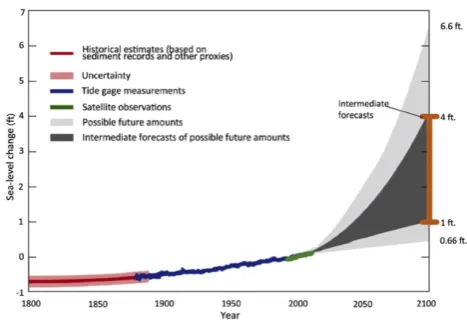
N recent years, the problem of the mean sea level increase has attracted a lot of attention from the scientific community [1] Fig. 1 shows estimated, observed, and predicted global sea levels from 1800 to 2100. Estimates from proxy data drawn in red between 1800 and 1890, pink band shows uncertainty. Tide gauge data is depicted in blue for 1880 - 2009. Satellite observations are shown in green from 1993 to 2012. The future scenarios range from 0.66 ft to 6.6 ft in 2100. This, in particular, results in increase of average floods all over the world [1]. Potential for use of social vulnerability assessments to aid decision making for the Colorado dam safety branch [2]. Furthermore, increased population enhances the severity of the flood aftermaths. It is estimated that within 2050 the population will be increased by 130 million, which will demand for a huge increase of water reservoirs.
Manuscript received July 26, 2018; revised August 1, 2018.
K B Bittumon is with the University of Genoa, Genoa, 16145 Italy (e-mail: [email protected]).
Dr. M.V. Ivanov is with the Bauman Moscow State Technical University, Moscow, 105005 Russia (e-mail: [email protected]).
O.A. Ivanova is with the Bauman Moscow State Technical University, Moscow, 105005 Russia (e-mail: [email protected]).
Prof. R. Revetria is with University of Genoa, Genoa, 16145 Italy (corresponding autor phone: +390103532866; email: [email protected])
K V Sunjo is with the University of Genoa, Genoa, 16145 Italy (email: [email protected])
Nowadays a lot of attention is devoted to catastrophic floods. Due to their rarity, they cause much greater local floods can cause significant damage to the national economy. In addition, due to the growing population of the Earth, there is the need to develop new territories that have not historically been inhabited, for example, due to the increased risk of floods.
[image:1.595.312.546.320.484.2]At the same time, regular floods are much better studied and forecasted, so it seems possible to concentrate on management water release in order to improve the safety of the adjacent territories.
Fig 1. Estimated, observed, and predicted global sea level rise from 1800 to 2100. (Redrawn from Melillo et al., 2014)
II. LITERATURE REVIEW
Since 1960 various system modeling tools have been developed to use extensively in hydroelectric generation and water management. The study focusing on a non-traditional simulation models has been developed by Forrester in the sixties at MIT [3]. System dynamic models involve simulation and optimization algorithms to develop planning programs [4]. Since dynamic modeling allow to evaluate the effect of any change over time, simulation models have become the primary tool of hydro hydropower modeling system. Under a given set of conditions, simulation model can result in the response of a system. Classical simulation models can be divided into water balance method and mass balance method. Mass balance models are best for water management, using flow routing to determine release from reservoirs or system of reservoirs. System dynamics uses a conceptual tool for creating dynamic behavior of complex system. A system dynamic model for multiple reservoir hydropower operation was first developed. Models focused on real time operation of hydropower systems have been created by means of many tools such as Powersim, STELLA,
K.B. Bittumon, M. Ivanov, O. Ivanova, R. Revetria, K.V. Sunjo
Modeling for the Safe Management of Complex
River Basins
iThink, Exted, and Venisim. Some model includes managing hydraulic structure operational modes to ensure safety from flooding. Furthermore, a complex approach of modeling of a tandem reservoir system for drainage management gives optimal water to be drained with minimizing chance of flood keeping the effective power production [5,6].
Complex reservoirs water management may be performed basing on the analysis of water flow forecast (water volume, transition duration, max discharges and others), the existing water levels in the reservoirs, and the available receiving volumes. In any case the water management policy is developed in several steps. Firstly, a complete water demand plan has to be estimated with respect of its change with time. Secondly, technological constraints have to be set that would limit possible regulation of the water flow through the reservoir system. Finally, an optimal water discharge graph has to be constructed so that it would minimize flood risk, and meet the requirements of all stakeholders (power production plants, fisheries, ships’ navigation, agriculture and others) considering the developed water demand plan.
The second step is relatively easy implemented as long as all relevant data regarding the water reservoir system has been provided. However, it is much more complicated to correctly assess all the stakeholders as far as increasing its number will result in complication of the water reservoir management model. Therefore, most of the known management models limit the constraints with power production.
Optimization of energy management and conversion in the multi-reservoir systems based on evolutionary algorithms [7]. In many cases considering a single constraint may not be enough and an additional parameter is introduced. This could be maintaining required energy production while minimizing water pollution while water allocation for agriculture use, meeting water demands in severe conditions, i,e, in drought, or minimizing flood risks and aftermaths, and many others [8,9,10,11,12]. In some cases, up to three different constraint may be set. Considering more constraints simultaneously is performed very rarely as this significantly complicates the known model and increases the computation time.
Based on the aforesaid, the aim of this paper is to develop a multi-criteria model for dam management at a complex river basin that would consider required power production while minimizing flood risks and maintaining certain water level in the basins.
Up to now, many approaches to modelling to support water policy management of complex reservoir systems have been proposed. Most of them commonly use a Monte Carlo optimization [13, 14]. It performs optimization over long period of time (several centuries) of historical or synthetically generated discharges. However, optimal management policies may not be applied to any other time series among the one that was calculated. Another widely used approach is based on linear programming, which is often combined with Monte Carlo simulation [15]. The main disadvantage of this method is that all mathematical apparatus has to be linear or linearizable. Another approach is based on the representation of a river network through a set of nodes and links, which is called a network flow optimization. Nodes represent reservoir and links – channels and flows. Such approach is even faster than the others. One of the first attempt to introduce this
approach at Missouri river is reported in [16], where it shown that even a simple river basin is very complex to be modelled using this approach when many constraints are considered.
Methods based on linearization may encounter a number of diffculties to be applied precisely due to its large scale or the lack of precision. In these cases a nonlinear programming models might be applied. Nowadays they are considered to be the most advanced due to its power and robustness. However due to its nonlinearity there is always a risk for a model not to converge. Another widely used and well studied approach is dynamic programming [17]. Dynamic programming tools decompose an original task into a several sub tasks, i.e. split with time, which can be solved separately. This approach may be easily used for a multi-constraint system and is very robust. However, it requires a careful selection of the initial data that will be analyzed and may be very difficult to extend to large river systems.
Other approaches are based on explicit stochastic optimization. In all cases optimization is performed without knowledge of the forecast. The modelling may be done using stochastic linear programming, stochastic dynamic programming, and stochastic optimal control. Such approaches require high computational capacities and thus may be hardly applied for large river basins. The last one, on the contrary, may be easily applied for large scales, however does not provide high precision in calculations. Another stochastic optimization approach is multiobjective optimization model. It allows setting many simultaneous constraints with subjective weights (relative magnitude of importance). In [18] this method is analyzed with four objectives: maximize energy production, improve energy production quality, minimize water discharges for water supply and maximize reliability of water supply.
III. GEOMORPHOLOGY OF VALLE D’AOSTA
The region Valle d’Aosta accounts for an important share of hydropower network system in Italy, consisting of mountainous region situated in North Western Italy bordered by Switzerland and France. Around 20% of this area is less than 1500 meters from main sea level. Fig.1 shows the region of interest Valle d’Aosta. In actual practice the region consist of glaciers and snowpack in winter determine the runoff regime characterized by minimum flow values in winter and maximum flows in spring and summer. The principal river of the valley is 100 km through the whole Region between Courmayeur (near the Mont Blanc) and Quincinetto, (near the Pont St Martin) the outlet of the valley. The ice covers 5.5% of the total area and a great number of lakes are located in Valle d’Aosta. Some of such lakes are artificial and are used for the regulation of hydropower production. The availability of water to be stored in a certain elevation provides favorable conditions for hydroelectric production. In the year 2011 the hydroelectric network capacity of the region was about 900 MW with a power production of 2743 GWh per year.
maximum flow of water available for the turbines and by an energetic coefficient that represents the actual power produced in MW. For each reservoir the maximum height must be provided for finding the power produced in each plant. Finally, the maximum flow and the time of concentration must be inserted for the dam and rivers connecting each other. These data, together with the initial and final conditions for the reservoir capacities, complete the conceptual model of the system.
Fig.2. Topological map of Valle d’Aosta with terrain
The elevation and availability of water leads the network of reservoirs to function effectively. The Fig 2 shows the topology of the region with terrain reflects the need for controlling the flow buy a simulation and optimization preventing flood without affecting power production.
IV. MODELING
Hydroelectric power plants may be located either in parallel to each other or in series. In this paper, it was selected a combination of two parallel reservoirs (A) and (B) and one installed in series after the parallel ones (C) in a way that the outlet water flow from reservoirs (A) and (B) falls into the third reservoir (C). (Fig. 3). Such a combination is considered to be one of the simplest for calculation but at the same time very commonly used.
Fig. 3. A general scheme of reservoirs connection
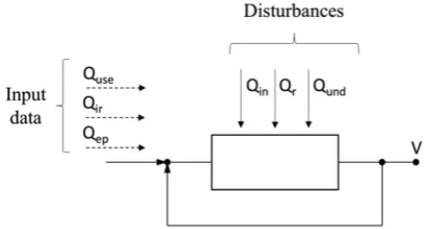
In the very general case, the water balance model for each reservoir may be described as follows (see Fig. 4). The reservoir is supplied by the input stream from the upstream
[image:3.595.310.551.211.329.2]channels (Qin). Additionally, rainwater (Qr) is taken into account. The transition of underground water (Qund) is also considered through the reservoir bed in positive (inside the reservoir) and in negative (to the ground) directions. Water may outgo from the reservoir due to evaporation (Qev), consumption for agricultural needs (Qirr) and household maintenance (Quse). In the lower tail of the channel, the water is involved in the process of electricity generating (QEP) and may be discharged through the bypass (Qbp) in order to increase the rate of emptying the reservoir. A sum of QEP and Qbp in total gives the output flow (Qout).
Fig. 4. Water flow model through a single reservoir
However, at this stage in the developed model evaporation is not considered because its calculation is complicated and will be added later. Therefore, the balance equation may be defined as follows:
𝑄
"#+ 𝑄
%± 𝑄
'#(− 𝑄
"%%− 𝑄
'*+− 𝑄
+,− 𝑄
-,= 0
, where:𝑄
"# - incoming flow𝑄
% – atmospheric precipitation𝑄
'#( - underground water (could be positive or negative)𝑄
"%% - water, spent for irrigation𝑄
'*+ - water for household and industrial usage𝑄
+, - discharge for energy production𝑄
-, - discharge through bypassAs was stated in the literature review the modelling was performed with a model predictive control (MPC) method. The simulation model is shown on Fig. 5.
[image:3.595.49.293.625.741.2] [image:3.595.307.545.627.755.2]
The input data consists of the water amount required for household usage, irrigation and power production. A set of data including incoming flow due to rain precipitation, underground flows, and flow from the upstream reservoir represents a sum of all disturbances.
In order to perform an efficient water management, two strategies have been developed: an operating strategy and a planning strategy.
Operating strategy was developed with a simulation horizon 10 hours, and moving horizon 3 hours.
As inputs were set
𝑄
"%% - water, spent for irrigation,𝑄
'*+ - water for household and industrial usage,𝑄
+, - discharge for energy production:𝑢
"=
'2 '3 '4 '5 '6 '7 '8 '9 ':
,
where:
𝑢
;, 𝑢
=, 𝑢
> -𝑄
'*+ for 1st, 2nd and 3rd reservoirs, respectively;𝑢
?, 𝑢
@, 𝑢
A -𝑄
"%% for 1st, 2nd and 3rd reservoirs, respectively;𝑢
B, 𝑢
C, 𝑢
D -𝑄
+, for 1st, 2nd and 3rd reservoirs, respectively. Also, a “pattern matrix” has to be entered, which consists of demand water supply:𝑢
;;⋯ 𝑢
;F⋮
⋱
⋮
𝑢
#;⋯ 𝑢
#F ,where
𝑗 ∈ 1, 𝑚
and𝑚
- simulation horizon;𝑖 ∈ 1, 𝑛
and𝑛
- number of inputs (demands).For each input its minimum (
𝑢
"OPQ)
and maximum (𝑢
"OST) values are defined, so that “pattern matrix” can change only within these limits:𝑢
"∈ 𝑢
"OPQ, 𝑢
"OSTAs disturbances were set
𝑄
"# (incoming flow),𝑄
% (atmospheric precipitation),𝑄
'#( (underground water):𝑑
"=
(2 (3 (4 (5 (6 (7 (8 (9 (:
,
where:
𝑑
;, 𝑑
=, 𝑑
> -𝑄
"# for 1st, 2nd and 3rd reservoirs respectively;𝑑
?, 𝑑
@, 𝑑
A –𝑄
% for 1st, 2nd and 3rd reservoirs respectively;𝑑
B, 𝑑
C, 𝑑
D -𝑄
'#( for 1st, 2nd and 3rd reservoirs respectively. So, the “disturbance matrix” may presented as follows:𝑑
;;⋯ 𝑑
;F⋮
⋱
⋮
𝑑
V;⋯ 𝑑
VF ,where:
𝑗 ∈ 1, 𝑚
and𝑚
- simulation horizon;𝑖 ∈ 1, 𝑘
and𝑘
- number of disturbances.Incoming flow for 3rd reservoir is calculated as follows:
𝑄
"#4= 𝑄
+,2+ 𝑄
+,3+ 𝑄
-,2+ 𝑄
-,3, where:𝑄
+,2, 𝑄
+,3 – discharges for energy production in 1st and 2nd reservoirs respectively;
𝑄
-,2, 𝑄
-,3– bypass from 1st and 2nd reservoirs respectively. For underground water flows a random matrix is created so that
𝑄
'∈ 𝑄
'OPQ, 𝑄
'OST .Discharge through bypass is a variable value, so it can be changed up to a certain maximum.
The elevations of reservoirs in region shown in network diagram of Valle d’Aosta (Fig. 2.) The first step is to be making a conceptual model based on the given network. Each hydropower plant is characterised by a number of parameters such as minimum and maximum level of reservoir, flow rates, power produced. In addition to this describing the initial and final values required for each reservoir is also specified, completes the conceptual model.
We can consider a general case of hydroelectric power plant in order to understand the conceptual modelling because the region consists of 32 reservoirs mutually connected and we have to consider each dam separately before connecting it to a single network. Generally the reservoir has three levels of capacity shown in Fig. 6, which are as follows: dead storage level (DSL, i.e., water level below which no electricity generation is possible), normal headwater level (NHL, i.e., accepted level in reservoir), surcharged reservoir level (SRL, i.e., water level aimed to store water during rainy season. In our case, we are considering only two basic levels the DSL and NHL. The reservoir will receive water from different sources like precipitation, ground water and water inflow from upstream reservoir.
Fig.6. A reservoir representing different levels of water based on constraints. SRL- Surcharged Reservoir Level, NHL- normal Head water
level and DSL – Dead storage Level.
The management of hydroelectric power plant can be characterised by several constraints. Our main aim is to prevent from the overflow of water which results in the collapse of dam and this is prevented by maintaining a mass balance on each node and at each time interval.
So, in general and depending on boundary conditions we have to account for:
2. optimal mode of operation for maintaining the NHL. 3. production of rated power.
The software can be useful to compare different scenarios arising, for example, by a change of climatic conditions, or by different management politics. In this work, analysed scenario of water availability and simulation is done for a period of one year with an interval of one hour. The computer model begins with defining rated capacity, rated flow rate, rated power and head at which the plant works. In order to fulfil the boundary conditions an equation governing the flow rate has to be input which will keep the capacity of the reservoir within the DSL. Also, a mass balance is created by adding or exiting a specified flow rate according to our rated value. This constraint will limit the capacity within the DSL i.e. the minimum level will be returned to zero when capacity of reservoir reaches the minimum limit of dam.
Fig.7. Water movement in a reservoir Beauregard (a segment in Valle d’Aosta)
The reservoir Beauregard is specifically analysed (Fig. 7). In the above equation we can find the dependence of minimum limit on flow rate and energy production based on flow rate, head and efficiency. All the variables are treated as constants because in our case they are used defined. A 10% of capacity is made for all the reservoirs and efficiency is considered to be 81%. But from the network we can clearly see that the power production cannot be maintained to the optimum value i.e. rated value because the capacity is decreasing with respect to time. So, in order to solve this here
we are considering a mass balance on each power plant based on the flow rate at which it works.
Similarly, all other 31 reservoirs are modelled and balanced Fig. 8. This mass balance can be assumed to be rainfall or from other resources which we took as a general case as flow- in our work, it may also from the exit of turbine to the next reservoir. Wide arrow indicates the direction of water course and thin arrow indicates the logical and structural relationship between the operators and flow chart elements. Next step is to cascade all this separately modelled power plant into a single network. This is accomplished by calling each separately modelled plant to a single network by using slice variable tool in Powersim. Subsequently we can simulate the obtained network for a period of one year from 2018 to 2019 with a time interval of one hour. Thus, the model is verified after one run of simulation. On interconnection some reservoirs will be affected with overflow or exceeding the SRL. This is slashed by creating a by-pass from the reservoir to the water channel.
V. RESULTS
The proposed case study of Valle d’Aosta was modelled and successfully simulated in Powersim. It results in the creation of a real multi cascade river network and ensured the water release from each dam based on the considered constraints. The major inputs shall include the following:
1. reservoir DHL and NHL levels 2. reservoir storage capacity 3. rated flow rate from reservoir 4. head of reservoir
5. efficiency of power plant.
After entering all the required data and initial conditions we can simulate the model by clicking a suitable button on the relevant control panel. The results are plotted in the Fig. 8. Graphical representation of simulation for a period of one year and we can see that the capacity of each reservoir is in its rated value i.e. it is maintained constant for each run and hence the modelled is verified and a balanced flow rate is obtained. The overall annual production is found to be 265.355 GW.
We can generate a dependence of power produced from each reservoir based on its capacity and it is plotted in excel by importing the simulated results into it shown in Fig. 9.
Fig.9. Showing capacity and power produced of reservoirs in Valle d’Aosta
The model of the considered river network may be used to optimize a number of decisions concerning the management of the plant on the overall. For example, a simple goal may be that of maximizing the hydroelectric generation under the satisfaction of safety conditions. Thus, optimization cannot be separated by a careful risk analysis.
VI. FUTURE ASPECTS
The simulation performed gives maximum power which can be produced annually without uncertainties. In actual practice this may lead to uncontrolled distribution of water causing flood threatening life and investments. Balance flows of incoming flow, evaporation, and underground aquifers flows, bypass, reservoir, irrigation and domestic uses are taken into account. Each of these contributions can be represented with empirical formulae. In case of excessive accumulation the bypass which acts preventing structural failures. Based on such a modeling framework, optimization can be fruitfully applied for an effective management of the reservoir operations. As pointed out in [6,7] typical goals may be the following:
1. maintaining sufficient head leaves in reservoir to avoid the uncertainty of failure and flood due to overflow over spillways;
2. excluding the electricity consumption and storage, assumed complete consumption of produced power without wastage;
3. reducing the risk of flood by limiting the discharge flow of reservoirs.
By varying at different levels of consumption of water resources downstream such as domestic, agricultural, and electricity generation needs results effectively water management. Localized storage in agricultural fields can be implemented as a secondary means.
A sensitivity analysis can be done after an optimization or a risk analysis by implementing an actual uncertainty with highest probabilities an optimized reservoir control is possible.
Among the various approaches for water flow optimization, here we focus on genetic algorithms. Though they are not well developed yet and require vast monitoring set, high computing capacity, and help of an “expert” to "educate" their application, genetic algorithms appear to be
appropriate in our context for various reasons. First of all, they do not require additional information such as the derivative of the cost or high-order derivatives. Thus, their application is straightforward inside in simulation tool like Powersim and, in principle, they allow to escape from local minima. By contrast, no guarantee to the convergence to the global point of optimum is ensured.
VII. CONCLUSION
Modeling of hydroelectric systems with economic objectives are mostly difficult, it requires understanding the complex relationship between load market system and social safety. The model developed provide basis for an operational policy through numerous runs of simulation model throughout one year. This work is a way to develop powerful and transparent models to address hydroelectric generation systems of long term planning that are well-suited to being optimized. Optimization may aim at efficiently managing the reservoir operations to maximize the income from the power market and keep the river network far from flood. The key success of any optimization problem is its effective implementation based on the system features by using suitable mathematical model and proper algorithms. In the management of hydroelectric generation system, there are lots of uncertain and complex information. Future research should explore the use of uncertain information in system dynamics simulation.
VIII. ACKNOWLEDGEMENT
The authors would like to thank Angelo Alessandri for some helpful comments.
REFERENCES
[1] Melillo, Jerry M., Richmond, Terese (T.C.), Yohe, Gary W. (Eds.), 2014. Climate Change Impacts in the United States: The Third National Climate Assessment. U.S. Global Change Research Program.
[2] Ferre, L.E., Mc Cormick, B., Thomas, D.S.K, 2014 Association of State Dam Safety Officials Annual Conference 2014. Dam Saf. 2014 (2), pp. 664-684.
[3] J. Forrester, 1961. Industrial Dynamics. M.I.T. Press, Cambridge, Mass.; Wiley, New York.
[4] Chen, H H. and Wang L. 1987. “Hydropower Simulation: An Overview. Waterpower'”. pp. 803 -812.
[5] R. Revetria, L. Damiani, M. Ivanov, O. Ivanova, 2017, “An Hybrid Simulator for Managing Hydraulic Structures Operational Modes to Ensure The Safety of Territories With Complex River Basin from Flooding” Proceedings of the 2017 winter Simulation Conference. [6] R. Revetria , O. Ivanova, K. Neusipin, M. Ivanov, M. Schenone, L.
Damiani, 2017, ”Optimization Model of a Tandem Water Reservoir System Management” Proceedings of the World Congress on Engineering and Computer Science 2017 Vol II WCECS 2017, October 25-27, 2017, San Francisco, USA.
[7] Omar J. Guerra, Gintaras V. Reklaitis, 2018, Advances and challenges in water management within energy systems, Renewable and Sustainable Energy Reviews, Volume 82, Part 3, pp. 4009-4019. [8] Claus Davidsen, Suxia Liu, Xingguo Mo, Peter E. Holm, Stefan Trapp, Dan Rosbjerg, Peter Bauer-Gottwein, 2015, Hydroeconomic optimization of reservoir management under downstream water quality constraints, Journal of Hydrology, Volume 529, Part 3, Pages 1679-1689, ISSN 0022-1694,
https://doi.org/10.1016/j.jhydrol.2015.08.018.
rainfall, Ecological Indicators, ISSN 1470-160X,
https://doi.org/10.1016/j.ecolind.2017.09.026.
[10] Jafar Y. Al-Jawad, Tiku T. Tanyimboh, 2017, Reservoir operation using a robust evolutionary optimization algorithm, Journal of Environmental Management, Volume 197, pp. 275-286, ISSN 0301-4797, https://doi.org/10.1016/j.jenvman.2017.03.081.
[11] Daniel McInnes, Boris Miller, 2017, Optimal control of a large dam using time-inhomogeneous Markov chains with an application to flood control, IFAC-PapersOnLine, Volume 50, Issue 1, pp. 3499-3504, https://doi.org/10.1016/j.ifacol.2017.08.936.
[12] Gokcen Uysal, Bulut Akkol, M. Irem Topcu, Aynur Sensoy, Dirk Schwanenberg, 2016, Comparison of Different Reservoir Models for Short Term Operation of Flood Management, Procedia Engineering, Volume 154, pp. 1385-1392, ISSN 1877-7058,
https://doi.org/10.1016/j.proeng.2016.07.506.
[13] Krzysztof Postek, Dick den Hertog, Jarl Kind, Chris Pustjens, 2018, Adjustable robust strategies for flood protection, Omega, ISSN 0305-0483, https://doi.org/10.1016/j.omega.2017.12.009.
[14] Gaofeng Zhu, Xin Li, Jinzhu Ma, Yunquan Wang, Shaomin Liu, Chunlin Huang, Kun Zhang, Xiaoli Hu, 2018, A new moving strategy for the sequential Monte Carlo approach in optimizing the hydrological model parameters, Advances in Water Resources, Volume 114, pp. 164-179, ISSN 0309-1708, https://doi.org/10.1016/j.advwatres.2018.02.007.
[15] Hiew, K. 1987. ‘‘Optimization algorithms for large scale multi-reservoir hydropower systems.’’ PhD dissertation, Dept. of Civil Engineering, Colorado State Univ., Ft. Collins, Colo.
[16] Lund, J., and Ferreira, I. 1996. ‘‘Operating rule optimization for Missouri River reservoir system.’’ J. Water Resour. Plan. Manage.,122(4), 287–295.
[17] Young, G. 1967. ‘‘Finding reservoir operating rules.’’ J. Hydraul. Div., Am. Soc. Civ. Eng., 93 (6), 297–321.