Abstract— Resource-constrained project scheduling models
either the single-mode or the multi-mode case finds minimum schedule that minimizes the completion time of a project with constant per period renewable resource. That the level of provided resources, each period must be constant, does not reflect a real-life situation and hence makes these models inappropriate for solving project delays and abandonment. We present a Hybrid resource-constrained project scheduling problem (Hybrid RCPSP), the single-mode case and the multi-mode case for solving delays and abandonment of projects. These models are combination of the existing single-mode and multi-mode RCPSP models with some added assumptions. Our method essentially formulates the network project as a Hybrid RCPSP (single-mode or the multi-mode) and then finds the minimal schedule that minimizes the completion time of the project using priority rule based scheduling technique, while the level of the renewable resource availability varies. The idea is that if a completion time of the project can be minimized then, that project cannot be delayed or abandoned.
We performed our method on a real-life building construction project (a fenced three-bedroom bungalow), a fictitious single-mode and multi-single-mode network projects. Our result of the real-life building construction project, show that to solve project delays and abandonment, the level of per period available resource should vary and our result of the fictitious Single-Mode and Multi-mode RCPSP show that no matter how small (even at zero level in some time periods), the per period amount and how long the length of the period, the projects will not be delayed or even abandoned
Index Terms— Construction Projects, Network Analysis,
Project Scheduling, Resource Constraints
I. INTRODUCTION
ON- preemptive single-mode resource-constrained project scheduling problem (single-mode RCPSP) finds the minimal schedule that minimizes the total completion time of a project, while satisfying the precedence and the resource constraints. The precedence constraint ensures that a job cannot be started until all its direct predecessors are completed, while the resource constraint is the limitations of the renewable resources required to accomplish the activities (jobs, tasks).
Manuscript received July 10, 2017; revised July 29, 2017.
P. I. Adamu is with the Department of Mathematics, Covenant University, Ota, Nigeria.
O. T. Aromolaran is with the Department of Computer and Information Science, Covenant University, Ota, Nigeria
F. A. Aitsebaomo is with the Nigerian Building and Road Research Institute,, Ota, Nigeria
The extension of the single-mode RCPSP to real life situation is the multi-mode RCPSP. Here, the different ways, called modes of performing each job is considered, and each job is performed in one of them. Therefore, a mode is the different ways of combining different levels of resource requirements with a related duration. Three types of resources (Slowinski [7]) are used, the renewable, non-renewable and doubly constrained resources. The non-renewable resources have limited per-period availability (e. g. the number of skilled workers needed daily is limited) and the non-renewable resources are limited for the entire project (for example the total money needed for the project is limited). Doubly constrained resources are limited both for each period and for the whole project, but are not considered separately. This is because when the sets of the renewable and non-renewable resources are enlarged the doubly constrained resources are indirectly considered.
This problem has found application in many real life applications and industries, such as project management and crew scheduling, construction engineering, production planning and scheduling, fleet management, machine assignment, automobile industry and software development. However, this problem has been shown to be an NP-hard optimization problem shown in [4] if the number of non-renewable resources is more than one. Hence exact methods become intractable as the number of activities and the number of modes for each activity increases [8]. Therefore large – real world problems of this class can only be tackled by heuristics, for example see [3].
Within the single-mode and the multi-mode RCPSP the per period renewable resource is constant, which does not reflect real-life situations. This makes these models not suitable for solving delays and abandonment of projects which is majorly a practical problem.
Hence in this paper we propose a model, we call Hybrid RCPSP (either the single-mode or the multi-mode) to solve delays and abandonment of projects. Hybrid RCPSP is the combination of the existing RCPSP (either the single-mode case [10] or the multi-mode [2] [9] with some assumptions. The added assumptions are: (1) the level of renewable resource should vary to reflect true life situations. (2) The period should be allowed to vary. (For example, if the project owner was bringing in funds monthly and now wants it to be weekly or quarterly) (3) All purchases should be done before any job execution starts.
We formulate the project as a Hybrid RCPSP (either the single-mode or the multi-mode) and then use a priority rule based scheduling technique to find the minimal schedule that minimizes the completion time of the project. The Earliest Finish Time (EFT) rule and the Serial Schedule Generation Scheme (SSGS) are used as the priority rule and the
Solving Project Delays and Abandonment Using
Hybrid Resource-Constrained Project
Scheduling Models
Patience Imoh Adamu, Olufemi T. Aromolaran , and Francis A. Aitsebaomo
schedule generation scheme respectively. The main idea is to determine if the completion time of a project is able to be minimized which translate that the project cannot be delayed or abandoned. The contributions of this study include:
A solution method for solving project delays and abandonment.
Propose a Hybrid RCPSP (either the single-mode or the multi-mode).
Formulation of a real life construction project as a hybrid single-mode RCPSP.
We ran our method on different problems including a practical building construction project (a fenced three-bedroom bungalow), a fictitious single-mode and multi-mode network projects. The real-life building construction project was formulated as Hybrid-single-mode RCPSP and the chart of the model show that to minimize delay and abandonment of projects, the available renewable resource should be varied. Solving the fictitious single-mode and multi-mode network project using different levels of per period amounts, showed that no matter how long is a period and no matter how reasonably small is a level of per period available resource, the projects proceed to completion stages. All these experiments showed that projects may not be unnecessarily delayed or abandoned if they are formulated as Hybrid RCPSP.
II. PRELIMINARIES AND RELATED WORKS
A. Resources for Resource-Constrained Projects
Slowinski [7] and Weglarz [12] categorized the resources (e. g. manpower, materials, equipment, capital etc.) needed for the execution of a project into three categories:
Renewable Resources: These are resources that are made available per period (hourly, daily, weekly, monthly, etc.). For each period for instance every day, the quantity of each resource for instance manpower, made available is assumed constant. For example, a company can decide to make available 10 skilled and 20 unskilled laborers on a daily basis for the execution of a particular project until it is completed. That is, the quantity of each resource is renewed every period. (It is this class of resources that is used for the Hybrid single-mode RCPSP, whose model we are using to solve the project abandonment problem).
Nonrenewable Resources: These are resources whose
availabilities are not limited per period, but on the total project. For example, an individual may decide that the building project must not be more than a particular amount of money (say, X dollars). Which means money to be spent is limited to the total project basis. This is the budget for the project. Again the individual may decide to use 50 skilled and 120 unskilled laborers for the total project. This implies that the total availability of manpower is also limited.
Doubly Constrained-Resources: These are resources that are
limited both on total project basis and on per period basis. Money falls into this category because, apart from having a budget for a project, the per-period cash flows are also limited. If the renewable and non-renewable resources are enlarged appropriately, the doubly constrained resources are already considered. Hence, in the model only the renewable and non-renewable resources are explicitly considered.
B. The Description of the Single-Mode RCPSP model
The resource-constrained project scheduling problem (RCPSP) considers a single project with J number of jobs (j
= 0, 1, 2, 3,…, J, J+1) to be performed, where job j = 0 corresponds to a unique dummy source ( project start) and job j = J+1 corresponds to the unique dummy sink (project end). Dummy jobs are appended only if there is no unique start and end jobs naturally. Two types of constraints exist between jobs: the precedence constraint and the resource constraint. The precedence constraint delays the performance of a job until all its immediate predecessors (Pj) are completed. That is, a job cannot start processing
unless all its direct predecessors (Pj) are completed. In the
resource constraint, the jobs require resources to be processed, but the availability of each resource is limited. There are K types of renewable resources (k = 1, 2, 3, , , K.) Each resource type k has constant per-period availability of
Rkt (for example every week Y dollars is made available for
the project), and each job uses r j,k units of resource type k to
be processed every period of time. Once job j starts processing, there is no interruption and its processing time is pj. For both start and end jobs j = 0 and j = j+1, their
processing times dj= 0 and their resource usage rj,k = 0 for all
k. The objective is to find precedence and resource feasible schedule that minimizes the makespan (total completion time) of the project.
A conceptual formulation of the scheduling problem by Talbot and Patterson [10] is as follows:
where Fj denotes the completion time of job j; a vector of
finished times of the jobs, denoted by {F1, F2, ... ,Fn } is
called a schedule and A(t), the set of jobs undergoing processing at time t. The objective function (1): minimizes the finish time of the last job of the project, which minimizes the total completion time of the project. Constraints (2): the precedence constraint ensures that the start time of job j is greater than the finished time of all its predecessors (Fh). Constraints (3): demands that in time t,
the resource constraint enforces that the total resource demands of the jobs under processing A(t), should not be greater than the limit for each resource type k. Constraint (4): ensures that the finished times of every job j, Fj is
greater or equal to zero. It defines the decision variables. Blazewicz et al. [1] showed that RCPSP belongs to the class of NP hard optimization problems. Hence, solving large problem instances owe themselves only to heuristic solution methods.
C. The Description of the Multi-Mode RCPSP model
The Multi-Mode RCPSP is an extension of Single-Mode RCPSP. In the Single-Mode RCPSP each job is considered to be done in only one way as we can see in the model above, whereas in Multi-Mode RCPSP, the different possible ways each job can be performed is considered. For example, in a building construction, the project owner may decide to buy the already made blocks (bricks) from the block industries or decide to buy the materials and have the blocks molded to reduce cost . These two methods of obtaining blocks have different levels of resource requirements and different durations. This is called the mode of each job which is the different ways of combining different levels of resource requirements with related durations. So each job may be
𝑖𝑛𝑖 𝑖𝑧 𝐹𝑛+1 (1)
Subject to:
Max
𝑛𝜖 𝑃𝑗
{ 𝐹𝑛} + 𝑗≤ 𝐹𝑗; ∀ 𝑗 = 1, 2, ⋯ 𝑛 + 1; 𝑛𝜖𝑃𝑗 (2)
𝑟𝑗 ,𝑘 ≤ 𝑅𝑘𝑡; 𝑘𝜖𝐾; 𝑡 ≥ 0
𝑗𝜖𝐴 𝑡 (3)
executed in one of the prescribed ways (modes, ) depending on the performance criterion of the problem. Whereas in Single-mode RCPSP only renewable resources are used, in the Multi-Mode RCPSP both renewable and non-renewable resources are used. The objective of Multi-Mode RCPSP as Single-Multi-Mode RCPSP is to find the schedule of activities subject to the precedence and resource constraints that minimizes the completion time (makespan) of the project. A description and the Integer programming formulation for this model have been developed by Talbot [9] and Hartmann [2]
D. Priority Based Project Scheduling Technique
This technique constructs precedence and resource feasible project schedules. It is made up of a priority rule and a schedule generation scheme. The priority rule lists the jobs of the project in a topological order while the schedule generation scheme finds the finished times of each job (schedule) using the activity list. There is quite a number of existing priority rules (Vanhoucke[11]). They used different information on the project as job priorities. Examples include: Shortest Processing Time (SPT) which uses the processing times of the jobs to determine the job priority, Minimum Slack (MSLK) uses the logic of the network to know which job to choose and Greatest Resource Work Content (GRWC) which uses the project resource information, and so on.
There are only two Schedule Generation Scheme (SGS) available: the serial SGS and the parallel SGS [5]. In constructing their schedules, the serial SGS selects an activity and then schedules it at its earliest precedence and resource feasible finished time while the parallel SGS schedules the jobs at their schedule times.
E. Local Search Procedure
The local search procedure (Hartmann 1997) converts a multi-mode case to a single-mode case. The procedure is used to generate a feasible mode assignment
⋯ for all the jobs, 𝑗 𝑗 ⋯ 𝑗 .
A mode assignment is first generated randomly for each job in the project. Then the sum of their nonrenewable resource requirements, is calculated for each nonrenewable resource type 𝑖 ⋯ . If this sum exceeds the available nonrenewable resource level 𝑖 ⋯ , it implies that the mode assignment is infeasible and a simple mode assignment strategy is employed to improve the current mode assignment: A job is randomly selected and a mode, different from its current mode. This leads to a another mode assignment Then check if the sum of their nonrenewable resource requirements exceeds the available nonrenewable resource level 𝑖 ⋯ . If yes, choose another mode for that job and repeat the process. This process is continuously repeated until the mode assignment becomes feasible.
When the mode assignment is feasible with respect to non-renewable resources, the multi-mode case becomes the single-mode case.
III. THE HYBRID RCPSP
A. The Hybrid Single-Mode RCPSP
The hybrid single-mode RCPSP is a combination of the existing single-mode RCPSP (Talbot and Patterson [10])
and the added assumptions. So the conceptual formulation of this problem is:
where constraint (4) is a mathematical representation of the assumption (i) below. It demands that in time t, the resource constraint enforces that the minimum resource demand of jobs in the eligible set (E(t) is the set of jobs whose predecessors has been scheduled) in time t, be not greater than the limit of each resource type k given in that period. This ensures that in every period that work is to be done, the resource provided should be enough to execute at least one job.
B. The Hybrid Multi-Mode RCPSP
The hybrid multi-mode is a combination of the existing multi-mode RCPSP (Talbot [9]; Hartmann [2]) with the added assumptions. Constraint (4) is a mathematical representation of assumption (i) below.
where, J is the number of jobs. K, the number of renewable resources. I, the number of non-renewable resources.
𝑅 , the level of available renewable resource k in time t.
, the total available budget of non-renewable resource i The objective function (1) minimizes the completion time of the project. Constraint (2) makes sure that exactly one mode and one completion time is assigned to each job. Constraint (3) takes care of the precedence relations between jobs, while (4) ensures that the minimum resource demand of jobs in the eligible set in time t, is not greater than the limit for each resource type k given in that period. (5) guarantees that the non-renewable resource availability is not exceeded. This problem is NP-complete (Kolisch and Drexl [6]) and real world problems as the one we are tackling now can only be solved using heuristics.
C. The Added Assumptions
(i) The level of the per period resource be allowed to vary from time to time, but may not be less than the minimum resource requirement of any job in the eligible set of jobs, if work will be done in that period.
𝑖𝑛𝑖 𝑖𝑧 𝐹𝑛+1 (1)
Subject to:
Max
𝑛𝜖 𝑃𝑗
{ 𝐹𝑛} + 𝑗≤ 𝐹𝑗; ∀ 𝑗 = 1, 2, ⋯ 𝑛 + 1; 𝑛𝜖𝑃𝑗 (2)
𝑟𝑗 ,𝑘 ≤ 𝑅𝑘𝑡; 𝑘𝜖𝐾; 𝑡 ≥ 0 𝑗𝜖𝐴 𝑡
(3)
𝐦𝐢𝐧 𝒓𝒋,𝒌≤ 𝑹𝒌𝒕; ∀𝒋𝝐𝑬 𝒕 ; 𝒌𝝐𝑲; 𝒕 ≥ 𝟎 (𝟒)
𝐹𝑗 ≥ 0 (5)
𝑖𝑛 𝑡. 𝑥𝑗 𝑡 (1) 𝐿𝐹𝐽
𝑡=𝐸𝐹𝑗 𝑗
=1
𝑥𝑗 𝑡 = 1; 𝑗 = 1, ⋯ , 𝐽 (2) 𝐿𝐹𝐽
𝑡=𝐸𝐹𝑗 𝑗
=1
𝑡. 𝑥ℎ 𝑡 ≤ 𝑡 − 𝑗 𝑥𝑗 𝑡; 𝑗 = 2, ⋯ , 𝐽; ℎ𝜖𝑃𝑗 𝐿𝐹𝐽
𝑡=𝐸𝐹𝑗 𝑗
=1
(3)
𝐿𝐹ℎ
𝑡=𝐸𝐹ℎ ℎ
=1
𝒎𝒊𝒏 𝒓𝒋𝒎𝒌≤ 𝑹𝒌𝒕; 𝒌𝝐𝑲 ; ∀𝒋𝝐𝑬𝒕 ; 𝒕 ≥ 𝟎 (𝟒)
𝑗 𝑖𝑥𝑗 𝑡 𝐿𝐹𝑗
𝑡=𝐸𝐹𝑗 𝑗
=1 𝐽
𝑗 =1
≤ 𝑖; 𝑖𝜖 (5)
This assumption is necessary to take care of the situation where the project owner may want to increase or reduce the level of per period available resource for convenience. The effect is that anytime the available amount is changed, the remaining jobs are simply rescheduled using the recent level of available renewable resource. This will only vary the completion time of the project.
(ii) The period allowed vary from time to time.
For
example, the project owner may have been providing the funds monthly, and now wants it to be weekly or even quarterly (every three months). The effect again is the same as per period availability. The remaining jobs are simply rescheduled using the new period. Again the project completion times varies accordingly.
(iii) All the materials needed for executing the jobs may
be purchased where possible before job execution starts.
D.
The Method of Solution
Our method for solving delays and abandonment of projects does the following:
1) Formulates the project as a hybrid- RCPSP, either as a single-mode case or a multi-mode case,
2) Uses a priority rule (Earliest Finish Time priority rule) to find the activity list of the jobs,
3) Uses a schedule generation scheme (Serial Schedule Generation Scheme (SSGS)) to find the schedule each time the level of available resource changes, thereby knowing the completion time of the project.
IV. EXPERIMENTS
1. Formulation of A Fenced 3-Bebroom Bungalow as
a Hybrid Single Mode RCPSP
This is a real life situation data from Nigeria Building and Road Research Institute (NBRRI), Ota, A branch of the Federal Ministry of Science and Technology, Nigeria. The main data has 71 jobs making up this construction project. The bill of quantity and material schedule was used to prepare the activity listing whose summary is in Table 1. We assume that all the materials are purchased before the execution of any job. To reduce the main data so that it can fit into a page, some of the jobs were grouped together. For example, the job, “Roofing” contains five jobs: bending reinforcement for
[image:4.595.309.535.70.301.2]roof beam, form work for roof beam, casting of roof beam, framing of carcassing and placing of the roof covering, while the job “finishing”, contains eight jobs: internal and external rendering, floor screeding, laying of wall and floor tiles, placing of ceiling covering, fixing of electrical sub-circuit and fixing of sanitary appliances. The constructed network of the 3-bedroom bungalow with a fence can be seen in Figure 1 while Figure 2 shows how the cost of the project is distributed with time.
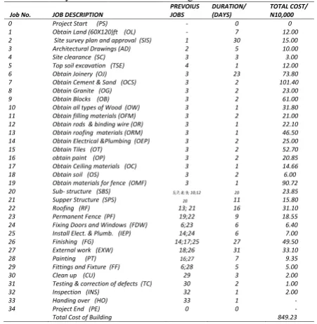
Table 1: Activity list of the 3-bedroom bungalow
[image:4.595.305.550.434.613.2]The second column of Table 1 contains the job description. The fourth column has the estimated duration in days of each job. The last column contains the total cost per N10,000 (ten thousand naira) of each job. Total cost includes the cost of materials and cost of labor for both skilled and unskilled labors as at Feb. 2017 in Nigeria. By this, we are able to calculate approximately the total cost of a fenced three-bedroom Bungalow in Nigeria, which is almost N8, 492,300 (eight million four hundred and ninety-two thousand, three hundred naira) as at February, 2017. The network was constructed to know the topological order of the jobs.
Fig. 1: Network for the Fenced 3-Bedroom Bungalow
Fig. 2: The distribution of the cost of the project
Job No. JOB DESCRIPTION
PREVOIUS JOBS
DURATION/ (DAYS)
TOTAL COST/ N10,000
0 Project Start (PS) - 0 0
1 Obtain Land (60X120)ft (OL) - 7 12.00 2 Site survey plan and approval (SIS) 1 30 15.00 3 Architectural Drawings (AD) 2 5 10.00
4 Site clearance (SC) 3 3 3.00
5 Top soil excavation (TSE) 4 1 12.00
6 Obtain Joinery (OJ) 3 23 73.80
7 Obtain Cement & Sand (OCS) 3 2 101.40
8 Obtain Granite (OG) 3 2 23.00
9 Obtain Blocks (OB) 3 2 61.00
10 Obtain all types of Wood (OW) 3 1 31.80 11 Obtain filling materials (OFM) 3 2 21.00 12 Obtain rods & binding wire (OR) 3 1 22.10 13 Obtain roofing materials (ORM) 3 1 46.50 14 Obtain Electrical &Plumbing (OEP) 3 2 25.00
15 Obtain Tiles (OT) 3 2 52.70
16 obtain paint (OP) 3 2 20.85
17 Obtain Ceiling materials (OC) 3 1 14.66
18 Obtain soil (OS) 3 2 6.00
19 Obtain materials for fence (OMF) 3 1 90.72 20 Sub- structure (SBS) 5;7; 8; 9; 10;12 20 23.85
21 Supper Structure (SPS) 20 11 15.80
22 Roofing (RF) 13; 21 16 31.10
23 Permanent Fence (PF) 19;22 9 18.55
24 Fixing Doors and Windows (FDW) 6;23 6 6.40 25 Install Elect. & Plumb. (IEP) 14;24 6 7.00 26 Finishing (FG) 14;17;25 27 49.50 27 External work (EXW) 18;26 31 33.10
28 Painting (PT) 16;27 7 9.35
29 Fittings and Fixture (FF) 6;28 5 5.00
30 Clean up (CU) 29 3 2.00
31 Testing & correction of defects (TC) 30 2 1.00
32 Inspection (INS) 32 1 2.00
33 Handing over (HO) 33 1 -
34 Project End (PE) 0 0 -
Total Cost of Building 849.23
THE NETWORK OF A FENCED 3_BEDROOM BUNGALOW
9
8
4 2.
1. 20. 21
12 6. 14
3
13 7
5.
19
17
18
6
PS 22. 23.
24 25
26.
27.
32 29.
31
30. 28
33.
[image:4.595.307.523.638.764.2]Figure 2 shows that the jobs with high cost are concentrated at the beginning of the process. This is expected because all the materials are bought before job execution starts. In building construction, for example, the bulk of the money spent, is usually on buying the materials, as labor is relatively cheap in this part of the world, Nigeria. Scheduling these jobs gives us an idea of the minimum amount needed per period, if work will take place in that period. This graph buttresses our assertion that per period resource availability should be varied, which does not only address the real life situation, but also makes projects not be abandoned or unnecessarily delayed.
This formulation helps the project owner to know the total cost of the project approximately and the minimum approximate amount needed every period for work to be done in that period. For example, from the network, we observe that job 1(obtaining land for the project) comes first and its total cost is N120, 000 (one hundred and twenty thousand naira) and it duration is 7 days. So this informs the project owner that the minimum amount needed for the first 7 days is N120, 000. This is done before the commencement of any job execution, which makes the project owner to plan financially before commencement.
2. Fictitious Examples
Experiment 2a
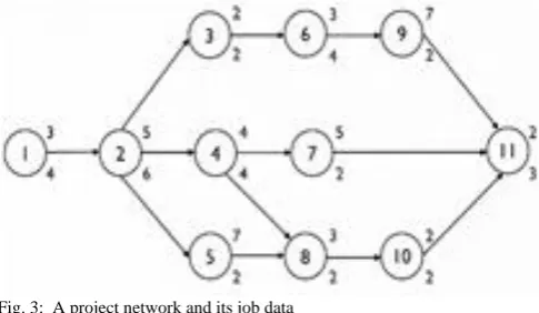
[image:5.595.304.550.292.769.2] [image:5.595.48.291.403.544.2]We used the fictitious example of a single-mode RCPSP (Vanhoucke 2012) to explain our method. Figure 3 and Table 2 explains the problem.
[image:5.595.46.280.537.699.2]Fig. 3: A project network and its job data
Table 2: A project with eleven jobs.
Experimental set up
In this example the number of renewable resource type is one (K=1). The experiment is to schedule the jobs with different levels of renewable resource in different periods. We examined two situations where resources were provided in all the time periods and where resources were not
provided in at least one period. That is, we have (a) Available resource per period = {4, 6, 8, 8, 6, 4, 3} and (b) Available resource per period = {{4, 0, 6, 2, 8, 6, 4, 2, 4, 4, 3}. The zero level means that theproject owner was not able to provide any resource that period.
We used a priority based project scheduling technique to find the schedule in every stage to know the jobs to be performed in that stage and their completion times. We used the earliest finish time (EFTj) priority rule to find the
activity list and used the Serial Schedule Generation Scheme (SSGS) to construct the schedules for different levels of available renewable resource in each period.
Results:
In this experiment renewable resource was provided throughout the periods but at varying levels. That is
{4, 6, 8, 8, 6, 4, 3}. Using EFT priority rule, the activity listing is {1, 2, 3, 4, 6, 5, 7, 8, 9, 10, 11}. Then to find the schedule, using serial schedule generation scheme (SSGS) as follows: In every stage we schedule the jobs with the provided resource in that period.
Stage 1
g = 1; t = 0; Eligible Job E1 ={J1}; Given level of
Renewable Resource R1 = 4 units. Scheduled job S1 =
J1; Finish Time of J1 = 3; Remaining Resource (R’t = Rt
– rj / R’1 = 4 – 4 = 0). Scheduled Job is J1; Scheduled
Jobs SJ = {J1}
Stage 2:
g = 2; t = 3; E2 = {J2}; R2 = 6; S2 = J2; F2 = 8; R’2 = 6-6
= 0. (Job 2 is scheduled). SJ = {J1, J2} Stage 3:
g = 3; t = 8; E3 = {J3, J4, J5}; R3 = 8;
(a) g = 3a; S3a = J3 (using list); F3 = 10; R’3a = 8 –
2 = 6.
(b) g = 3b; t = 8; E3b = {J4, J5, J6}; R’3b = 6; S3b = J4
(J4 can still be scheduled here because
remaining resource is 6); F4 = 12; R’3b = 6 – 4
= 2.
Because of resource constraint and precedence constraint J6 cannot be scheduled here but J5 can be
scheduled. (Job 3 and Job 4 are scheduled in this stage).
SJ = {J1, J2, J3, J4} Stage 4:
g = 4; t = 12; E4 = {J5, J6, J7}; R4 = 8;
(a) g = 4a; S4a = J6; F6 = 15; R’4a = 8 – 3 = 5
(b) g = 4b; schedule time t = 8 or 12 (because at t = 8, R’3b = 6 – 4 = 2); E4b = J5, J7, J9; t
= 8; S4b = J5; F5 = 15.
(c) So at t = 8, R’3 = 0; at t= 12; R’4 = 8 – 6 =
2. Hence J7 can still be scheduled at t = 12.
G = 4c; S4c = J7; F7 = 17. (Job 6, Job 5 and Job 7 are
scheduled in this stage).
SJ = {J1, J2, J3, J4, J6, J5, J7}. Stage 5:
g = 5; t = 15; E5 = {J8, J9, J11}; R5 = 6; R’3 = 6 – 2 = 4;
S5a = J8 and S5b = J9; R’5 = 0; F8 = 18; F9 = 22. (Job 8
and Job 9 are scheduled in this stage). SJ = {J1, J2, J3, J4, J6, J5, J7, J8, J9}
Stage 6:
g = 6; t = 17; E6 = J10, J11; R6 = 4; R’6 = 4 – 4 = 0; no job can
be scheduled here
Job No. Previous Jobs Duration/weeks Resource Req.
1 - 3 4
2 1 5 6
3 2 2 2
4 2 4 4
5 2 7 2
6 3 3 4
7 4 5 2
8 4; 5 3 2
9 6 7 2
10 8 2 2
g = 6; t = 18; E6 = J10, J11; R6 = 4; R’6 = 4 – 2 = 2; S6 = J10;
F10 = 20; R’6 = 0. (Job 10 is scheduled in this stage). SJ =
{J1, J2, J3, J4, J6, J5, J7, J8, J9, J10} Stage 7:
g = 7; t = 22; E7 = J11; R6 = 3; S7 = J11; F11 = 24; R’7 = 3 – 3
= 0. (Finally Job 11 is scheduled in this stage) SJ = {J1, J2, J3, J4, J6, J5, J7, J8, J9, J10, J11}.
Summary:
The provided resources {4, 6, 8, 8, 6, 4, 3} every period, gives {3, 8, 10, 12, 15, 15, 17, 18, 22, 20, 24} as the job schedule and the total completion time of the project as 24 weeks. Fig. 4 shows the schedule of the example project of Fig. 3 and Table 2.
.
Fig. 4: Project schedule with varying level of renewable resources
The example project was formulated as a hybrid single-mode RCPSP and a priority rule based scheduling technique was used to solve it and we got a completion time 24 weeks.
Experiment 2b
We examine another situation where the units of the provided renewable resource have a zero level. That is {4, 0, 6, 2, 8, 6, 4, 2, 4, 4, 3}. The activity listing is the same as above.
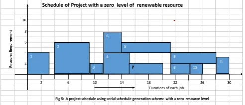
[image:6.595.307.514.172.258.2]Using the same SSGS above The schedule is {3, 9, 11, 15, 21, 14, 20, 24, 28, 26, 30} and the total completion time of this project is 30 weeks. Fig. 5 shows the schedule.
Fig. 5: Project schedule with zero level of renewable resource
We observe in Fig. 5 that in the third week after the first job was scheduled no funds was provided, so there was no work done. In the fourth week 6 units was provided, so the remaining jobs were scheduled to know the job(s) to be executed in that week. It can be seen that job 2 can be done in the fourth week without violating the precedence and the resource constraint. This reflects true life situation which we see only leads to the increase in the completion time of the project and not abandonment.
In both cases, the project was not unnecessarily delayed. In the worst case scenarios, the completion times only get increased.
3. The Multi-Mode Case
A situation where the different ways of executing each job is considered, may be to reduce cost, is a multi-mode case. Below is a fictitious example. The 6-job project has 5 renewable resources and 1 non-renewable resource. Available resource in the first period for each renewable resource is 2, 4, 7, 1, N1000 and for second period is 2, 3, 5, 1, N1200. The total budget for the project is N4, 500. A period is assumed to be one week. See Fig. 6 and Table 3.
Fig. 6: Network for a 6-job project
Table 3:A fictitious example of a multi-mode project..
Result:
This case is solved by first converting it to a single-mode case using a local search procedure (Hartmann 1997) and solved using the priority based scheduling technique explained as experiment 2a above.
Solution to Project Example:
Using the mode assignment strategy for our example, a feasible mode assignment for the jobs is {𝑗 𝑗 𝑗 𝑗 𝑗 𝑗 because the sum of their
non-renewable resource (total cost) is N4, 400. This is now a single-mode case shown in Table 4.
Table 4: A single-mode case of the multi-mode 6-job project of Fig 6
Job(j) Mode(m) Duration(djm) Renewable Resource Demands (rjmk)
1 2 3 4 5(N)
1 1 3 1 1 4 1 N500
2 2 2 0 1 0 0 150
3 2 3 1 2 3 0 200
4 2 1 1 0 2 1 750
5 1 5 1 3 3 0 250
6 1 1 0 0 0 0 0
Available Resource in Period 1 2 4 7 1 N1000
Available Resource in Period 2 2 3 5 1 N1200
Using the method as in experiment 2a, the schedule is {3, 2, 3, 3, 8} and the completion time of this project is 8 weeks.
Schedule of Project with varing level of renewable resource
[image:6.595.46.292.221.322.2]Durations of each job Fig 4: A project schedule using serial schedule generation scheme with varying resource levels 10
26
2 6 10 14 18 22
R
es
o
u
rc
e
R
eq
u
ir
eme
n
ts
2 4 6 8
1 2
3 4
6 5
8 9
10 11
Schedule of Project with a zero level of renewable resource
[image:6.595.46.293.502.608.2]Durations of each job
Fig 5: A project schedule using serial schedule generation scheme with a zero resource level
10
R
e
so
u
rc
e
R
e
q
u
ir
e
m
e
n
t 8
6 4 2
26 30
2 6 10 14 18 22
1 2
3 4 6
5
8 9
10 11
1 1
3
4 2
5
6
Job(j) Mode(m) Duration(djm) Renewable Resource Demands (rjmk)
Non-Resource Demand (wjm1) (Total Cost)
1 2 3 4 5(N) 1 1 3 1 1 4 1 N500 1500
2 8 1 0 3 0 200 1600 2 1 4 2 3 2 0 250 1000 2 2 0 1 0 0 150 300 3 1 5 1 3 1 1 300 1500
2 3 1 2 3 0 200 600 4 1 4 0 1 3 1 400 1600
2 1 1 0 2 1 750 750 5 1 5 1 3 3 0 250 1250
2 1 1 1 6 1 100 100 6 1 1 0 0 0 0 0 0
Available Resource in Period 1 2 4 7 1 N1000 N4,500
[image:6.595.314.531.633.741.2]V. CONCLUSION
Delayed or abandoned projects (e, g, construction projects) as shown in Fig. 7 is a common sight in some parts of the countries of the world today and what to do to solve this problem is the motivation of this work.
We presented Hybrid-RCPSP models (single-mode and multi-mode), which is a combination of the existing RCPSP models (single-mode and multi-mode) and some assumptions. We performed experiments for a real-life construction project (a three-bedroom bungalow with fence), a fictitious single-mode network project and a fictitious multi-mode network project. Our results show that no matter how reasonably small is the level of per period available resource and how long the period, the projects are not delayed or abandoned which solves the problem of delays and abandonment in our societies.
[image:7.595.49.287.248.469.2]
Fig 7: Abandoned building construction projects
ACKNOWLEDGMENT
The support received from Covenant University, Ota, Nigeria is greatly appreciated.
REFERENCES
[1] J. Blazewicz, J. K. Lenstra,, and A. H. G. Rinnooy Kan,, “Scheduling subject to resource constraints: Classification and complexity”,
Discrete Applied Mathematics, vol. 5, 1983, pp. 11–24.
[2] S. Hartmann,”Project scheduling with multiple modes: A genetic algorithm”, Manuskripte aus den Instituten fur Betriebswirtschaftslehre der Universit at Kiel, no. 435, 1997. [3] S. U. Kadam and S. U. Mane, “A Genetic-Local Search Algorithm
Approach for Resource Constrained Project Scheduling Problem”,
International Conference on Computing Communication Control and Automation, Pune, 841-846. 2015
doi: 10.1109/ICCUBEA.2015.168
[4] R. Kolisch, “Project-Scheduling under Resource-constraints: Efficient heuristics for several problem classes”. Physica-Verlag, Hiedelberg; 1995.
[5] R. Kolisch, “Serial and Parallel resource-constrained project scheduling methods revisited – Theory and Computation”, European Journal of Operations Research, 90, 320 – 333, 1996.
[6] R. Kolisch, and A. Drexl, “Adaptive Search for Solving Hard Project Scheduling Problems,” Naval research Logistics, 43, 23-40. 1996. [7] R. Slowinski, Two Approaches to Problem of Resource Allocation
Among Project Activities: A Comparative Study, Journal of the Operational Research Society, 31, 711-723, 1980.
[8] A. Sprecher, and A. Drexl, “. Multi-Mode Resource-Constrained Project Scheduling Problems by A Simple General and Powerful Sequencing Algorithm” Journal of Operational Research, 107, 431 – 450. 1998
[9] F.B. Talbot, “Resource-Constrained Project Scheduling With Time – Resource Trade-Offs: The Nonpreemptive Case”, Management Science, 28(10):1197-1210. 1982.
[10] F.B. Talbot, J.H. Patterson,” An efficient integer programming algorithm with network cuts for solving resource-constrained scheduling problems”, Management Science 24 (1978) 1163-1174. [11] Mario Vanhoucke.( 2012). Optimizing regular scheduling objectives:
Schedule generation schemes. Pm Knowledge Center. [Online]. Available:
http://www.pmknowledgecenter.com/dynamic_scheduling/baseline/o ptimizing-regular- scheduling-objectives-schedule-generation-schemes.