On Gain Initialization and Optimization of
Reduced-Order Adaptive Filter
Hong Son Hoang Member, IAENG, and R´emy Baraille
Abstract—Despite all the progress in filtering algorithms for state estimation in very high dimensional systems, the technology is delicate and sometimes difficult to apply. Good initialization of filter gain, appropriate choice of tuning pa-rameters and their optimization are the key factors to achieve robust high-performance filtering algorithms. In this paper the authors propose a method for properly initializing the filter gain, and for efficient optimization of the filter performance. Numerical experiments will be given to illustrate the algorithm and to demonstrate the efficiency of the proposed filter for state estimation problems in classical low dimensional as well as in very high dimensional systems.
Index Terms—Adaptive filtering, data assimilation, dynam-ical systems, numerdynam-ical prediction, real Schur decomposition, stability.
I. INTRODUCTION
I
N a series of papers [1]-[5] a new technique known as a reduced-order adaptive filter (ROAF) is developed for solving the problem of state and parameter estimation in very high dimensional systems. The very high dimensional systems we mean here are those having the state vector of the dimension of order 106−107. Theoretically, thesetasks can be solved in the framework of the theory of Bayesian statistics, in particular, by the Kalman filter (KF) and/or its extensions [6]. However, application of the KF to very high dimensional systems is an extremely difficult task. Even under ideal conditions for applicability of the KF, its implementation is simply impossible due to insurmountable memory and computational requirements : it requires the solution of an enormous number of additional equations (order of 1012−1014).
To overcome the mentioned above difficulties, different approximation approaches are proposed among which the nudging, optimal interpolation, kriging, variational meth-ods ... [7]. To handle more general state and observation equations, the filters based on the sequential Monte Carlo approach like bootstrap filtering, the condensation algorithm, particle filtering, interacting particle approximations ... [8]-[11] are recently proposed and tested. Here the posterior probability density function is represented by a collection of random points. As the dimension of numerical model is very high, in all practically realizable algorithms one has
Manuscript received May 26, 2011; revised September 20, 2011. H.S. Hoang is with the Research Department, SHOM/HOM, 42 av Gaspard Coriolis 31057 TOULOUSE FRANCE email: [email protected]
R. Baraille is with the Research Department, SHOM/HOM, 42 av Gaspard Coriolis 31057 TOULOUSE FRANCE email: [email protected]
to reduce, explicitly or not, the set of estimated parameters. This is seen in the widely used variational approach [12], [13] where seeking an optimal trajectory in the phase space is replaced by finding an optimal estimate for the initial system state. For the class of sequential algorithms, the different approximate (or suboptimal) KFs algorithms were developed. These include, e.g., the Ensemble KF (EnKF, see [14],[15]) in which the covariance is approximated by a sample covariance estimated fromO(100) samples of the prediction and filtered errors and evolved according to the KF formalism. Another class of the Reduced-Rank KFs is proposed by [16].
The concept developed in the ROAF approach is to make reduction not of the model order [17] but of the dimension of the space spanned by the columns of the filter gain [2]. In such situation, the question on a filter stability is of the first importance. This issue has been studied in many works for the full KF, for example, in [18]. For the ROAF, as found in [3],[5], under detectability condition, it is possible to ensure a stability of the filter if the reduced-rank subspace is composed from unstable and neural eigenvectors (or singular vectors) of the system dynamics. For illustration of these results, see the experiments in [19]. In the light of the important requirement for stability of the ROF, it is strongly advisable to approximate the ECM in the full space in such a way that the space spanned by the columns of the ECM should cover the subspace of unstable eigenvectors or that of unstable singular vectors of the system dynamics.
The steps in the design of a ROAF are following: First a set of filters is chosen which are defined up to a vector of unknown parameters in the filter gain. Next the optimization is performed by adjusting the tuning parameters to minimize the mean prediction error (MPE) of the system output.
To better understand the basic features of the ROAF, in Table I the differences between two approaches, ROAF and Four-Dimensional Variational approach (4D-Var) [12] are presented.
It is evident that the performance of the ROAF depends on a selected class of filters and its parameterization. This paper will focus the efforts on the way to well initialize the filter gain and its parameterization. For example, in [4] the initial gain is chosen on the basis of the well-known Cooper-Haines filter (CHF) [20] whose gain is derived by assuming several physical hypotheses on water properties. The approach to be developed in this paper is numerically simple, more efficient and based completely on the numerical model. Another important contribution in the present work is to
IAENG International Journal of Applied Mathematics, 42:1, IJAM_42_1_04
TABLE I 4D-VARANDROAF
Approach 4D-VAR ROAF
Control vector Initial system state Gain parameters
Cost function Distance in phase space
MPE of system out-put
Optimization Batch-vector, iterative Sequential, SPSA
Gradient compu-tation
Integration of model and AE over assimi-lation period
Integration of model at each assimilation instant
demonstrate that it is possible to optimize the ROAF by two
time integration of the numerical model at each assimilation
instant. That is feasible due to introduced optimality in the MPE sense and the use of the simultaneous perturbation stochastic approximation (SPSA) algorithm. Compared to the 4D-VAR approach, this advantage is very significant since the latter requires a number of iterations (about 20), each of which includes one integration of the direct model and one backward integration of the adjoint equation (AE) of the tangent linear model (TLM), over all the assimilation period. In the section that follows, first a brief outline of the difficulties encountered in solving the filtering problems for very high dimensional systems as well as the algorithmic pro-cedure of the ROAF are given. The numerical propro-cedure for generating the samples of the prediction error (PE), proposed in [21], is described in section 3. These PE samples will participate in approximation or estimation of the parameters of the ECM needed in initialization of the filter gain. It is shown in section 4 that implementation of the ROAF is greatly simplified thanks to the SPSA algorithm. To illustrate all steps in the ROAF algorithm, first the classical problem on estimating the position and velocity of a vehicle based on position observations is considered in details in section 5. Application of the ROAF to high dimensional system is presented in sections 6-7 where the problem of estimation of the North Atlantic Ocean circulation using the satellite sea-surface height (SSH) is considered. The performance of the ROAF will be compared with that of the CHF studied in [4]. The conclusions are given in section 8.
II. ROAFAPPROACH
A. Kalman filter. Difficulties for high dimensional systems
Consider a standard filtering problem for linear time-invariant system
x(k+ 1) = Φx(k) +Bu(k) +w(k), k= 0,1,2, ... (1)
z(k+ 1) =Hx(k+ 1) +ǫ(k+ 1), k= 0,1,2, ... (2)
here x(k) is the n-dimensional system state at k := tk assimilation instant, Φ is the (nxn) fundamental matrix, B
is (nxm) matrix, u(k) is the m-dimensional known deter-ministic signal,z(k)is thep-dimensional observation vector,
H is the (pxn) observation matrix, w, ǫ are the model and observation noises. We assume w(k), ǫ(k) are uncorrelated sequences of zero mean and time-invariant covarianceQand
Rrespectively. Without loss of generality, for simplicity, let
B= 0. For the class of filters of the structure
ˆ
x(k+1) = ˆx(k+1/k)+K(k+1)ζ(k+1),ˆx(k+1/k) = Φˆx(k)
(3) whereζ(k+1) =z(k+1)−Hx(k+1/k)ˆ is the innovation vector,x(kˆ + 1)is the filtered (or analysis) estimate, x(kˆ + 1/k)is the prediction forx(k+ 1), the gain which will yield an unbiased minimum variance (MV) estimate for the system state is given by [22]
K(k+ 1) =E[ep(k+ 1)ζT(k+ 1)]E[ζ(k+ 1)ζT(k+ 1)] −1
(4)
E(.)is the mathematical expectation,ep(k+ 1) = ˆx(k+ 1/k)−x(k+ 1) is the PE for the system state x(k+ 1),
ζT(k+ 1) is the transpose ofζ(k+ 1). The gainK(k+ 1) takes the form
K(k+ 1) =M(k+ 1)HT[HM(k+ 1)HT +R]−1
(5)
whereM(k+ 1)is the ECM forep(k+ 1). The filtered error (FE) expressed by P(k+ 1) = E[ef(k+ 1)ef(k+ 1)T], e
f(k+ 1) := ˆx(k+ 1)−x(k+ 1)satisfies the Algebraic Ricatti Equation (ARE)
M(k+ 1) = ΦP(k+ 1)ΦT +Q, (6)
P(k+ 1) = [I−K(k+ 1)H]M(k+ 1).
The system of equations (3),(5),(6) constitutes the famous KF.
It is seen that for the state x(k) of dimension of order
106−107, it is impossible to apply the KF since the system
(6) in fact is composed from 1012 −1014 equations for
determining the elements of the matrix P(k)andM(k).
B. Full-order adaptive filter (FOAF)
Remark that in Eq. (3) all variables are well defined except the gainK(k). The idea in the FOAF [1],[2] is outlined as follows : 1) To introduce a new criteria of ”optimality” for the filter which relates directly its optimality to the choice of the gain; 2) This criteria should be such that it allows to design a low cost procedure for computing the optimal gain. Consider the filter (3) subject to a time-invariant gainK. Note that under mild conditions, the gainK(k)in the KF will converge in asymptotic to a constant gainK∞too. To satisfy the two mentioned requirements, first some q elements (or parameters) of the gain are selected which form a control vector to be optimized. The gain is supposed then to be
IAENG International Journal of Applied Mathematics, 42:1, IJAM_42_1_04
defined up to a vector of unknown parameters θ ∈ Rq satisfying
K=K(θ),the filters (3) are stable for all θ∈Θ (7)
The optimal gain is defined asK∗
=K(θ∗
)whereθ∗ is the solution of
J =J[θ] =E[Ψ(ζ(k))]→minθ,Ψ(ζ(k)) :=||ζ(k)||2 (8) here||.|| is thel2 vector norm. The optimal filter will be
MPE sinceζ(k)is a one-step prediction error. The algorithm of the FOAF is given in [2]. This algorithm requires to solve the adjoint equation (AE) associated with the TLM of the filtering Eq. (3). As the filter is stable and the forcing in the AE is nonzero only at the current assimilation instant, it is sufficient to make only a few iterations in the backward integration of the AE.
C. Structure of the gain
Selecting improper structures for the filter gain may lead to its instability and fast growth of estimation error : as the gain elements are functions of the random estimateθ(k), there is a high risk that the filter becomes unstable if no special gain structure is taken to ensure its stability during optimization process.
In [2] a ROF is introduced to reduce the number of unknown elements to be estimated in the filter gain,
xe(k+ 1) = Φexe(k) +Keζ(k+ 1) (9)
where Φe ∈ Rne×ne is the fundamental matrix of the equation for the reduced state xe∈Rne. By assumingx= Prxe, ne<< n,Pr ∈Rn×ne is given, the estimate for the full state xis recovered byxˆ=Prxˆe [23]. We have then
ˆ
x(k+ 1) = Φˆx(k) +Kζ(k+ 1), K=PrKe (10)
By this way, the number of unknown parameters in
Ke is dramatically reduced. From (9)(10) the correction Kζ(k + 1) is an element of the linear space R[Pr]. The choice of the operatorPr∈Rn×ne hence plays an essential role in providing the extent to which the filter can minimize the estimation error. The question on stability of the ROF is studied in [3],[5]. One of the simplest stabilizing gain structures is given by
K=PrΘKe, Ke=HeT[HeHeT +R] −1
, He=HPr, (11)
Θ = diag[θ1, ..., θne], θl∈(0,2)
A detailed study on stability of the ROAF [3] reveals that for ensuring its stability, the spaceR[Pr]should belong to a subspace spanned by the leading eigenvectors or Schur vec-tors of the system dynamics. Recently the similar conclusion has been proved in [5] for leading singular vectors of Φ.
III. NUMERICAL PROCEDURE FOR CONSTRUCTION OFPr If there is no difficulty in numerical computation of eigen-vectors for low-dimensional systems, the problem becomes unrealizable for the systems of state-space dimension of order 106-107. Determining characteristic polynomial of a
matrix by calculating its determinant is expensive. Compu-tation of determinant of(n×n)matrix requiresn3/3
multi-plications. Another difficulty concerns possible existence of complex eigenvalues. In addition, the problem of computing eigenvectors is unstable : small errors in specification of the initial matrix may result to large errors in estimation of the eigenvector and eigenvalue. As to the singular vectors approach, there exists an efficient Lanczos algorithm [24] for computing the leading singular vectors of very large sparse systems. The advantages of singular vectors approach are that they (singular vectors) are all real and their computation is numerically stable. However the computation requires the TLM and its adjoint code. The third approach dealing with leading real Schur vectors, enjoys all advantages of the singular vectors approach. Moreover, it does not require an adjoint code for the TLM. For these reasons in [21] a numerical procedure for generating the PE samples on the basis of DScVs (Dominant Schur vectors) is proposed. It is shown that the generated PE samples (referred to as DPE (dominant PE) samples) will develop in the direction of DScVs. These samples are very helpful for initializing the unknown parameters in the filter gain.
Compared to the ensemble-based filtering algorithms (EnBF) (see [14],[15]), we remark that if in the EnBF algorithms the PE patterns are sampled randomly according to the KF formalism, the procedure for simulating DPE samples (called DPE sampling procedure (SP-DPE)) is aimed at generating patterns to develop in the direction of rapid growth of the PE error (DScVs subspace). It is therefore not surprising that the gain is usually well estimated on the basis of an ensemble of small-size of DPE samples. In fact, from (4), the termE[ep(k)ζT(k)]maps the innovation vectorζ(k) into the space spanned by samples ofep(k). Secondly, the gain (7) stabilizes the filter (4) if the columns ofPr belong to a dominant Schur subspace ofΦ. Thus, the ”optimal” low-rank subspace for the gain is based on: 1) an ensemble of patterns of ep(k); 2) this ensemble should be as close as possible to a dominant Schur subspace ofΦ.
A. Sampling procedure based on orthogonal iteration method
The procedure for generating patterns developed in the direction of a dominant Schur subspace is proposed in [21]. Given an (n×L) matrix X0 with orthonormal columns, 1≤L≤n, the method of orthogonal iteration generates a sequence of matricesXi,
Si= ΦXi−1, XiGi=Si, i= 1,2, ..., (12)
IAENG International Journal of Applied Mathematics, 42:1, IJAM_42_1_04
whereXi is orthonormal. One sees that the columns of
Si:=Si(L) (13)
belong to the space spanned by the columns ofXi. Consider the Schur decomposition
XTΦX=T =diag(λ
i) + ¯N ,|λ1| ≥ |λ2| ≥...≥ |λn|
LetX= [X1, X2],X1isn×Lsub-matrix,N¯ is a block
upper triangular. Then roughly speaking the distance between
DL(Φ) := R[X1] andR[Xi] is of orderO(|λλL+1L |i)where R[Xi] denotes the linear space spanned by the columns of Xi (see [24], section 7.3)). Thus the orthogonal iteration method allows us to generate the columns ofXiapproaching the dominant LSchur vectors. In the future the columns of
Si = ΦXt−1 are referred to as DPE samples for the system
dynamics (1).
B. DPE sampling procedure [21]
Suppose we want to simulate T patterns for each of the first L Schur vectors of the system dynamics Φ. At the moment i = 0, i := ti, let xf(i) be an initial estimate for x(i). Suppose we are given the orthogonal matrix Xi, XT
i Xi=ILwhose columns areLorthonormal perturbations δxl
f(i), l= 1, ..., L.
Step 1. Fori≤T: Letxf(i)andXi be given. Integrate the modelL+ 1times for producingxp(i+ 1) = Φ(xf(i)) and x′l
p(i+ 1) = Φ(xf(i) +δxlf(i)), l = 1, ..., L. The new matrixSi+1(L) := [δx1p(i+ 1), ..., δxLp(i+ 1)] is performed
whose columns are
δxlp(i+1) = Φ(xf(i)+δxlf(i))−Φ(xf(i)), l= 1, ..., L (14)
Step 2. Apply the Gram-Schmidt orthogonalization
pro-cedure (see [24])Xi+1Gi+1=Si+1to the matrixSi+1. The
resulting orthonormal perturbations{δxl
f(i+1), l= 1, ..., L} are the columns of the matrixXi+1= [δx1f(i+1), ..., δxLf(i+ 1)].
Step 3. Ifi+ 1 > T: Stop the procedure. Otherwise set
i:=i+ 1 and go to Step 1 subject toxf(i+ 1)andXi+1. Comment 3.1. The SP-DPE algorithm can be applied to a
nonlinear system dynamics whereF(x)stays instead ofΦx
with the modification Φδx(i)≈F[x(i) +δx(i)]−F[x(i)]. The columns ofXi then tend to DScVs of the TLM.
Comment 3.2 By normalizing the columns of Xi+1, the
generated samplesSi+1 represent only the direction but not
the amplitude of PE. For the real physical problems the state vector may include different physical variables (layer thickness h, velocity (u, v), temperature T ...) and usually the filter is constructed first on the basis of the normalized variables (having a unit variance, for example). The columns of Si+1 then represent not real but normalized physical
variables. The non-normalized PE samples are obtained if we multiply the normalized ones by corresponding estimated
standard deviations. For simplicity of the presentation we keep the notationSi+1unchanged, understanding that
some-times they may be the results obtained through corresponding renormalization procedure.
Comment 3.3 The definition of xf(k+ 1) depends on whether it is applied in the off-line (SP1) or in the on-line (SP2) fashion. The off-line procedure assumesxf(k+ 1) := xp(k+1). On the other hand, by applying the SP-DPE during the filtering process, the on-line SP2 assumesxf(k) = ˆx(k), ˆ
x(k)is the filtered estimate, and it integrates the model from
ˆ
x(k)and its perturbed estimatex(k)+δxˆ l
f(k). The renormal-ization process can be performed then more precisely if there is a possibility to get some information on the ECM matrix
P(k)of the filtered erroref(k). ForP1(k)- square-root of P(k),P(k) =P1(k)P1T(k), the FE sample is obtained from
the relation δxl
f(k) =P1(k)δxlp(k), l = 1,2, ..., L. The PE patterns generated during assimilation process can be used to correct the ECM obtained by the off-line SP1 and to improve the performance of the PEF. In the future we will use the notations δˆxl
p(k) := δxlp(k) if the PE sample is generated by the on-line SP2.
C. Estimation of error statistics
Once the PE patternsSi =Si(L), i= 1,2, ..., T become available, they can be used to estimate error statistics or parameters of the ECM. For example, if all the elements of the matrixM have to be estimated, the following formula is appropriate for their estimation
M = 1 T
T
X
i=1
Bi, Bi:=SiΘξSiT = 1 L
L
X
l=1
δxlp(i)ξiδxl,Tp (i),
(15) In (15)Θξ=diag[ξ1, ..., ξN],ξi are given positive values or to be estimated during adaptation. For T > 1, L > 1, the term T1, L1 should be replaced by T−11,
1
L−1 to provide
an unbiasedness of the estimate. The filter with the gain constructed on the basis of the DPE patterns is referred to in the future as a Prediction Error Filter (PEF).
If it is easy to simulate an ensemble Si(L) with size L close or equal to the state dimension of small dimensional systems (see experiments with 2 dimensional system in section 5), serious difficulties arise when working with very high dimensional systems. Using L patterns with L << n
is insufficient for estimating the ECM. In such situation, the filter either diverges or produces rather poor estimates. It is therefore of interest to introduce in addition a ”reguralizing” term to compensate the lack of information contained in L
PE samples. We have then
Mα= (1−α)Ω(θ) +αM (16)
where Ω is a constant matrix of a given parameterized structure (see (19)), α ∈ [0 : 1] reflecting our confidence on Ω. The matrix M may be estimated using the samples generated by SP1 or SP2. The vector of parameters θ can
IAENG International Journal of Applied Mathematics, 42:1, IJAM_42_1_04
be chosen as a control vector to be adjusted to optimize the filter performance.
IV. SPSAALGORITHM
Return to the problem of finding the optimal vectorθ∗ to minimize the objective function (8). As there exist always uncertainties (due to initial and boundary conditions, system and observation noise statistics ...), computation of the gradi-ent of (8) becomes unrealizable. However, the gradigradi-ent of the sample objective function Ψ(.)can be evaluated at a given point θ = θ(k). Thus the vector θ can be adjusted during filtering process by applying the stochastic approximation (SA) procedure
θ(k+1) =θ(k)−Γ(k+1)∇θΨ(ζ(k+1)), k= 0,1, ... (17)
where∇θΨ(ζ(k+ 1))is the gradient ofΨ(.)with respect toθ computed atθ:=θ(k), Γ(k+ 1) is the factor ensuring a convergence of the algorithm (scalar or matrix) [25]. Compared to the KF, in the adaptive filter (AF) based on SA (17) no ARE is solved. Instead we have to integrate backward (one or few iterations) the AE whose cost is about two or three times greater than direct model integration.
It is a common fact, development of a discrete adjoint solver for partial differential equations requires a long time and it involves the errors resulting from necessary approximations used during the differentiation. With the recent progress in development of the SA algorithms, it is possible to perform the AF without requiring the adjoint code for the TLM as does the AF based on (17). This great computational saving becomes reality thanks to in-troducing a so called simultaneous perturbation stochastic approximation (SPSA) algorithm [26]. Such algorithm does not insist on direct measurements of the gradient of the objective function. Moreover, SPSA is especially efficient in high-dimensional problems in terms of providing a good solution for a relatively small number of measurements of the objective function. In such algorithms, all elements of
θl, l = 1, ..., q are randomly perturbed together to obtain two (possibly noisy) measurements of the sample objective function y(.) := Ψ(.) + µ where µ is a measurement noise, but each component gi(θk) of the gradient vector g(.) := ∇θΨ(ζ(k)) is formed from a ratio involving the individual components in the perturbation vector and the difference in the two corresponding measurements. For two-sided SP (Simultaneous Perturbation), we have
gi(θk) =
y(θk+ck∆k)−y(θk−ck∆k) 2ck∆ki
(18)
where∆ki can be chosen as the random variable having the symmetric Bernoulli (+/-) 1 distribution. Two common distributions that do not satisfy the conditions for ∆ki are the uniform and the normal. For sufficient conditions for convergence of the SPSA iterate (θk → θ∗) see [26]. The main conditions are thatak, ck both go to 0 at rates neither
too fast nor too slow, that J(θ) is sufficiently smooth near
θ∗
. As for ∆ki, they are independent and symmetrically distributed about 0 with finite inverse momentsE(|∆ki|−1) for all k, i. The advantage of the SPSA is that at each assimilation instant it requires only two measurements of the sample objective function to approximate the gradient vector regardless of the dimension of the control vectorθ(or maximally, three measurements if second-order optimization algorithms are used [26]). The SPSA approach is thus free from the need to develop a discrete adjoint of the TLM and its implementation cost is independent of the number of parameters to be optimized. It is therefore very appreciated for solving optimization problems in very high dimensional systems.
V. EXPERIMENT ON VEHICLE NAVIGATION A. State and observational equations
To be able to project the innovation directly on the subspace generated by the simulated DPE samples, and to show the ROAF as an efficient alternative tool for solving classical estimation problems, we present in this section the experiment with the very simple filtering problem considered in [27]. The system statex consists of
x(k) = (y(k), ν(k))T wherey(k)andν(k)are the position and velocity of the vehicle at instantk:=tk,∆t=tk+1−tk,
p(k+ 1) =p(k) + ∆tν(k) +1 2∆t
2u(k) +p−
(k),
ν(k+ 1) =ν(k) + ∆tu(k) +ν−
(k)
wherep−
(k)is the position noise, ν−
(k)is the velocity noise. The input u is the commanded acceleration. It is assumed that we are able to change the acceleration and measure the position every ∆t seconds
z(k+ 1) =p(k+ 1) +ǫ(k) =Hx(k+ 1) +ǫ(k)
In the state-space form (1),(2) we have
Φ = [φi,j]2i,j=1, φii = 1, i= 1,2;φ21= 0, φ12= ∆t, B =1
2∆t 2
, w(k) = (p−
(k), ν−
(k))T, H = (1,0)
The simulation is performed subject to the parameters in [27]: The position is measured with an error of 10 f eet
(standard deviation); The commanded acceleration is a constant 1 f oot/sec2; The position is measured 10 times
per second (∆t = 0.1). Thus the covariance matrices for
w, ǫare equal to
Q= [qi,j]2i,j=1, φ11= 10−6, φ12=φ21= 2x 10⁻⁵, φ22= 4x 10
−6,R= 100
IAENG International Journal of Applied Mathematics, 42:1, IJAM_42_1_04
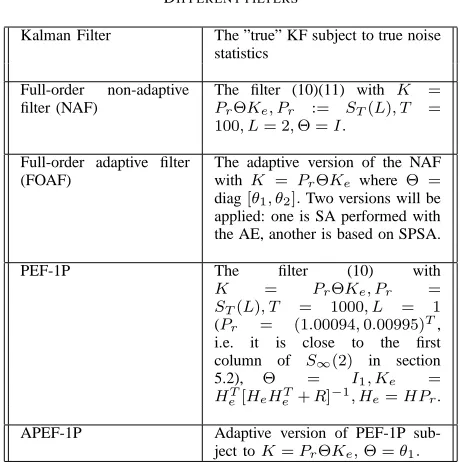
TABLE II DIFFERENT FILTERS
Kalman Filter The ”true” KF subject to true noise statistics
Full-order non-adaptive filter (NAF)
The filter (10)(11) with K =
PrΘKe, Pr := ST(L), T =
100, L= 2,Θ =I.
Full-order adaptive filter (FOAF)
The adaptive version of the NAF with K = PrΘKe where Θ = diag[θ1, θ2].Two versions will be
applied: one is SA performed with the AE, another is based on SPSA.
PEF-1P The filter (10) with
K = PrΘKe, Pr =
ST(L), T = 1000, L = 1 (Pr = (1.00094,0.00995)T, i.e. it is close to the first column of S∞(2) in section
5.2), Θ = I1, Ke =
HT
e[HeHeT+R]
−1
, He=HPr.
APEF-1P Adaptive version of PEF-1P sub-ject toK=PrΘKe,Θ =θ1.
The problem considered in this experiment is to estimate as accurately as possible the position and the velocity of the vehicle based on position measurements.
B. Kalman and different filters
[image:6.612.54.284.65.296.2]In Table II we summarize 5 filters to be performed in the experiment. Their performances will be compared.
Fig. 1 shows the components of the first column ofSt(2) and of the first Schur vector (first column of Xt(2)) in (12) produced during the SP-DPE procedure. One sees that the first components converge more quickly than the second ones. In the limit one finds
S∞(2) =
1 −0.1
0 −1 , X∞(2) =
1 0
0 −1 ,
G∞(2) =
1 −0.1
0 1 ,
and we have the identities
S∞(2) = ΦX∞(2), X∞(2)G∞(2) =S∞(2)
C. Numerical results
Evolution of the gain elementK1in the NAF, ROAF and
[image:6.612.312.551.302.474.2]KF is shown in Fig. 2. The curve ”FOAF-ADJ” corresponds to the FOAF with the gradient approximated by the AE whereas the curve ”FOAF-SP” is obtained on the basis of the SPSA algorithm. By construction the gain in the NAF is constant. The transition period for the Kalman gain is ob-served during the first 200 iterations. His value grows quickly since at the beginning one assumes that the initial estimation
Fig. 1. Orthogonal iteration algorithm: two components of the first vector of the PE matrix St(2) and that of the Schur Xt(2) resulting during iterations. The difference between the first components is more significant at the beginning of the iteration procedure and they converge more quickly in comparison with the second ones.
Fig. 2. Evolution of the gain elementK1 in NAF, ADJ,
FOAF-SP and KF. The Kalman gain becomes almost constant after about 200 iterations. The gains in two FOAFs have a stochastic character since they are estimated from the innovation vector. The curves SP” and ”FOAF-ADJ” behave similarly and have the same convergence tendency.
error is equal to zero corresponding to very small initialized ECM P(0). The gain in the FOAF is not smooth due to stochastic character of the innovation vector. One sees two curves ”FOAF-SP” and ”FOAF-ADJ” behave in the same way and they have the same convergence tendency which becomes more and more clear as assimilation progresses. If at the beginning (up to 150 iterations) two curves ”FOAF-SP” and ”FOAF-ADJ” are very similar, the amplitude of ”FOAF-SP” is rather greater afterward. Their fluctuations are strong at the beginning and attenuated thereafter. The gain coefficients in two filters KF and FOAF converge to different values.
Fig. 3 exposes the time averaged rms (root mean square) of the position errors produced by four filters. One sees that up to 30 sec the KF behaves better than the ROAFs
IAENG International Journal of Applied Mathematics, 42:1, IJAM_42_1_04
Fig. 3. Averaged rms of position error. The error level in the NAF is highest. Up to 30secthe KF behaves better but after this period its estimation error becomes higher compared to that of the FOAF-ADJ and FOAF-SP.
[image:7.612.55.313.58.234.2]Fig. 4. Averaged rms velocity error: Up to 30 secthe velocity error is higher in the KF compared to that of the ROAF. It becomes better estimated for the remaining of the assimilation period. The NAF produces the worse estimates for both position and velocity components
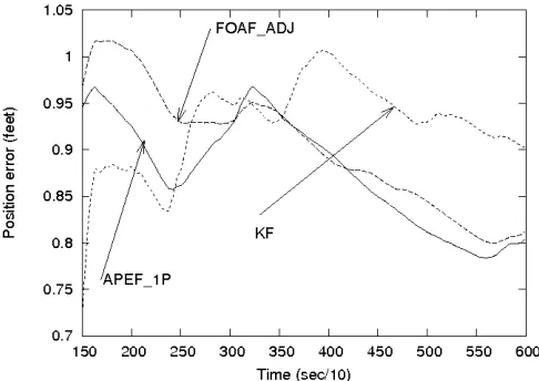
[image:7.612.50.289.290.461.2]Fig. 5. Averaged rms position error produced by the APEF-1P and other filters.
Fig. 6. Averaged rms velocity error produced by the APEF-1P and other filters. Reduction degrades only slightly the performance of the APEF-1P compared to that of the FOAF-SP.
but after this period its error becomes slightly higher. This is not true, however, for the velocity estimations: what we observe here is completely inverse to that already noted for the position errors. Fig. 4 shows that if up to 30 sec the velocity error is higher in the KF, it becomes lower for the remaining assimilation period. As to the NAF, it produces the estimates, for position and velocity components, with significantly higher errors, over all assimilation period.
To have the idea on how the order reduction influences on the filter performance, we have implemented also two filters PEF-1P and APEF-1P (see Table II for their description). One can check that for Pr = (1,0)T (the first column of S∞(2)), the PEF-1P with the parameterized gain is stable. Similar to Figs 3-4, the Figs 5, 6 present the rms errors for the position and velocity estimations produced by the FOAF-SP and APEF-1P. It is seen that order reduction degrades the performance of APEF-1P only slightly compared to that of FOAF-SP. Thus by projecting the innovation on the one-dimensional dominant Schur subspace it is still possible to design a high-performance ROAF for estimating the position and velocity of the vehicle.
VI. ALGORITHM OF THEROAFFOR ALTIMETRICSSH DATA ASSIMILATION
A. MICOM model and observations
The Miami Isopycnal Coordinate Ocean Model (MICOM), used here for the twin experiment is identical to that de-scribed in [4]. The model configuration is a domain situated in the North Atlantic from 300N to 600N and 800W to 440 W; for the exact model domain and some main features of the oceanic current (mean, variability of the SSH, velocity ...) produced by the model, see [4]. The grid spacing is about 0.20in longitude and in latitude, requiringN
h = Nx×Ny = 25200 (Nx = 140, Ny = 180) horizontal grid points. The number of layers in the model is Nz = 4. It is configured in a flat bottom rectangular basin (1860km×2380km×5km)
IAENG International Journal of Applied Mathematics, 42:1, IJAM_42_1_04
[image:7.612.50.293.527.699.2]driven by a periodic wind forcing. The model relies on one prognostic equation for each component of the horizontal velocity field and one equation for mass conservation per layer. We note that the state of the model is x:= (h, u, v)
where h = h(i, j, lr) is the thickness of lrth layer, u = u(i, j, lr), v =v(i, j, lr) are two velocity components. The layer stratification is made in the isopycnal coordinates, i.e. the layer is characterized by a constant potential density of water. Thus with three variables x:= (h, u, v), the state of the discretized model has the dimensionn= 302400.
The model is integrated from the state of rest during 20 years. Averaging the sequence of states over two years 17 and 18 gives a so-called climatology. During the period of two years 19 and 20, every ten days, we calculate the SSH from the layer thickness h which are considered as observations to be used for assimilation experiments (totally there are 72 observations). To be close to more realistic situation with the observations available only at along-track grid points, the observations are supposed to be available only at the points
i= 1,11, ...,131,j = 1,11, ...,171and are noise-free.
B. Reduced-order filter and gain structures
The filter used for assimilating SSH observations is
ˆ
x(k) =F[ˆx(k−1)] +K(k)Poiζ(k), k= 0,1, ... (19)
where x(k)ˆ is the filtered estimate for x(k), x(k) = [h(k), u(k), v(k)]is the system state atk:=tk,tk+1−tk= 10 ds (days), F(.) represents integration of the MICOM nonlinear model over 10 ds, K(k) is the filter gain, ζ(k)
is the innovation vector. As the observations are available not at all model grid points, the operatorPoiwill interpolate the missing SSH from observed points. Mention that in the KF this operation is performed automatically by the Kalman gain. The gain K is symbolically given byK=K1KhPoi, K1 := [I, GeTu, GeTv]T, Here ch := KhPoiζ(k) represents the correction for layer thicknesshusing the SSH innovation
ζ(k). As to Geu, Gev, they produce the correction for the velocity (u, v)from the correction ch using the geostrophy hypothesis. The operator Poi = Poi(ρ) = e−d/ρ interpo-lates the innovationζ(k) from observation points to all the grid points of the surface. Here d is the distance between two horizontal points, ρ is the correlation length. In the experiment we take ρ= 400km. As SSH observations are linear functions with respect to h, the observation equation is given by (3) (see [4]). By considering Poiz instead ofz, the observation operatorH is of the form
H= [Ip, ..., Ip] (20)
whereIpis the unit matrix of dimensionpxp(p=Nh). The parameterρ can be chosen as tuning parameter to optimize the filter performance.
C. Structure of the ECM for PE and its estimation
1) The caseα= 0: First assuming in Eq. (16)α= 0and
Mα=0= Ω = [ωl,m]Nl,mz=1⊗Ip, (21)
where⊗denotes the Kronecker product;Nzis the number of thickness layers in the model,ωlmis a scalar representing the covariance of the PE between two layers l and m. The elements ωlm can be chosen a priori from physical considerations or estimated from error patterns. For examp le, in the Cooper-Haines filter (CHF, see [4]), the elementsωlm are deduced from several physical constraints (conservation of potential vorticity, no motion at the bottom layer ...). In the PEF to follow,ωlm will be estimated using the patterns of DScVs. These patterns are generated by applying the SP1 which generate the sequence of ensemble of sizeL at each instanti:=ti, ti+1−ti= 10days(ds). Fori= 1, ..., T, the elementsωlm are estimated through
ωlm(T) = 1 T
T
X
it=1
¯ µit
l,m, (22)
¯ µit
l,m=
1
L
PL l=1µ
l,it
l,m, µl,it
l,m=
1
p
P
i,jδhlp(i, j, l;it)δhlp(i, j, m;it)
wherei, jspan all horizontal grid points whose number is equal top. The terms 1
T,
1
p should be replaced by
1
T−1, 1
p−1
for T > 1, p > 1 to provide the unbiasedness of the estimates.
In this paper, for illustrating purpose, we will apply the SA algorithms for seeking the (sub)optimal filters in two class of parameterized filters based on : 1) the CHF and 2) the PEF. The difference between the PEF and CHF is lying in the way we estimate the elements ofΩ. SubstitutingΩfrom (22) into (15) and forR(k) =σ2
rIp leads to
Kh= [k(1)Ip, ..., k(Nz)Ip]T, (23)
k(l) =PNz
m=1
ωl,m
s , s=PNz
m,m′=1ωm,m′+σ2r
hence k(l) is a scalar, l = 1, ..., Nz. The Cooper-Haines filter (CHF) [20] is obtained from (23) under three hy-potheses [4] : (H1) the analysis error for the system output is canceled in the case of noise-free observations ; (H2) conservation of the linear potential vorticity (PV); (H3) there is no correction for the velocity at the bottom layer. The AF in [4] is obtained by relaxing one or several hypotheses (H1)-(H3). For the noise-free observations, the parameterized gain in the CHF is of the form [4]
Kchf = [(θ1−θ2̺),(θ2−θ3)̺, ...,
(θNz−1−θNz)̺, θNz̺]
T⊗I
p. (24)
For the present MICOM model, ̺=−184.965[4]. The CHF, corresponding toθl= 1, l= 1, ...,4, has the form
IAENG International Journal of Applied Mathematics, 42:1, IJAM_42_1_04
Kchf = [185.965,0,0,−184.965Ip]T ⊗Ip. (25)
The adaptive filter in [4] is based on the parameterization (24) withθ1= 1 for noise-free observations.
2) The caseα6= 0: As seen from (22), by estimating the
matrixΩfrom SP1, the information on the filtered estimate and its estimation error are not taken into account. Moreover, as the elements ofΩrepresent only the covariances between different vertical layers, the horizontal structure of the PE is in fact completely ignored. These disadvantages can be compensated by putting α6= 0in (16). There are different ways to choose M in (16). For example, the samples from SP1 or SP2 can be used for estimating M on the basis of (15). When the samples are taken from SP2,M =M(k)is time-varying and the ECMMα=Mα(k)is updated during assimilation process. Mention that the formula (22) can be used also for updating M = M(k) with the patterns from SP2. The difficulty associated with application of (15) for estimatingM concerns the inversion of the innovation ECM
Σζ := HMαHT in the gain matrix (5). As the dimension of the observation vector is typically of order 104−105 ( p=Nh= 25200in the present MICOM model experiment), it is impossible to invert directly the matrix Σζ. At the present, iterative methods are widely used for finding x in the equation Σζx = ζ. For Σζ of very high dimension, iterative methods converge slowly, not to say on possible ill-posedness ofΣζ. In [21], by applying the Woodbury matrix identity [24], it is demonstrated that one can computeΣ−1
ζ ζ by inverting only the matrix of dimensions L×L whereL
is the size of the ensemble of PE samples.
D. Parameterization of the gain for the PEF. Adaptive filter
The parameterization of the gain for the CHF shown above takes the hypothesis on conservation of the linear PV as a departure point for parameterization (see (H2) for the CHF). This hypothesis implies that the vertical displacement interface (VDI) variables should be of (nearly) the same values. As shown in [4], working in the VDI space avoids to deal with the layer thickness variables (LTV)dh(k)since the latters have the values ranging from several tenths to thousand meters (depending on our interest in dividing the ocean depth in different layers). Optimizing the filter in the LTV space is hence undesirable due to the difficulty in determining to which extent each component θl should be allowed to vary during the optimization process.
Following the ROAF approach based on the gain structure (10)(11), we show now that it is possible to work directly in the LTV space and to define the allowable interval for each component θl. Using the Cholesky decomposition method, forMα=0= Ω (21), let
Ω =DDT (26)
[image:9.612.310.546.60.266.2]Subject to (26), the gain (11) can be parameterized as
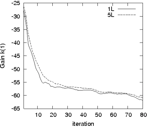
Fig. 7. Estimated gain coefficients at third layer as functions of iteration : the curves1Land 5Lcorrespond to applying the SP1 subject to two ensembles with sizeL= 1andL= 5at each instanti.
K=PrΘKe, Pr=D,Θ =diag= [θ1, ..., θNz], θl∈(0,2)
(27) wherePr = D,He = HD with Ke defined as in (11). Thus the diagonal elements ofΘcan be adjusted to minimize the prediction error for the SSH variable.
As the coefficientωlmrepresents the covariance of the PE between two layers l and m, they will be estimated in this paper from simulated DPE patterns as shown in (22).
The non-adaptive version (i.e. PEF) is obtained by setting
θl = 1, l = 1, ...,4. Once the estimates ωˆlm are available, the Eq. (23) can be used to calculate the gain of the PEF. For noise-free observations, σ2
r = 0, we obtained after 72 iterations the gain (subject toL= 1)
Kpef= [230.01,−84.97,−59.91,−84.13]T⊗Ip. (28)
Fig. 7 shows the estimated gain coefficients at third layer as functions of iteration during application of SP-DPE. Here we have applied SP1 (without assimilation) to simulate, at each time instanti :=ti, ti+1−ti = 10ds, two ensembles of samples of the size L = 1 and L = 5. The curves 1L
and5Lcorrespond to applying the SP1 subject to these two ensembles and Eq. (22). One sees that the coefficients are close one to other and there is a quick convergence of the gain coefficients. It means that for estimating the covariances between different layers, it is sufficient to simulate a se-quence of small size ensembles. The result in (28) shows that the coefficient at the first layer is of nearly the same magnitude compared with that of the CHF (25). The physical hypotheses (H2), (H3) in the CHF ignore the corrections for the intermediate layersl= 2,3. In the PEF these corrections remain important and play the important role in maintaining the better performance of the PEF (see next sections).
IAENG International Journal of Applied Mathematics, 42:1, IJAM_42_1_04
E. Adaptive filters based on CHF and PEF
The adaptive filters based on CHF and PEF will be used in further to assimilate the SSH observations. These filters (denoted as ACHF and APEF) are obtained by letting the vector of parametersθto vary to minimize the mean variance of the SSH prediction error. Let the initial values for θ be
θl =θl(0) = 1, l= 1,2,3,4 which correspond to the non-adaptive CHF and PEF. In the next section, as in section 5, two optimization algorithms based on AE and SPSA will be applied to updateθl.
VII. NUMERICAL RESULTS A. CHF and its modified versions
1) Efficiency of CHF: The CHF [20] is a simple, stable
assimilation scheme which is of relatively high-performance hence is used widely to assimilate the data into oceanic models. We run first the MODEL and CHF from the same initial guess state (climatology). The MODEL corresponds to running the MICOM model alone, without assimilation. It is seen from Table III that compared to the MODEL, the velocity errors in the CHF (eu(p), ev(p) and euv(p) correspond to the errors for the components u-,v- and total velocity (u, v)) are reduced by about 50%(more significant error reduction is observed for SSH, i.e. J). Here the RMS-PE of SSH is expressed incmand that of velocity - incm/s. Comparison of the results in column 3, Table III with that produced by the MODEL after the first assimilation instant (column 2, Table IV) confirms that simple integration of the model from the climatology increases the errors in all variables (see also Fig. 8 for the SSH error). It means that ocean modeling alone is insufficient for drawing the adequate knowledge on the oceanic circulation.
2) Improvement of CHF by exploiting horizontal structure of PE samples : In order to show that the PE samples are
very useful in improving the estimation of the ECM and to reduce the estimation error, let us modify the CHF by introducing the ECM (16) where Ω is the ECM leading to the CHF gain (25). As to the matrix M, it is estimated fromLdominant PE samples generated by SP1 and through application of (15), i.e. the columns of ST(L) at T = 50. This modified filter is denoted as MCHF(HORIZ). Fig. 9 displays the variance of SSH prediction error resulting from the CHF (curve ”CHF”) and MCHF(HORIZ) (curve ”CHF-HORIZ-10L”) in which L = 10. One sees that the modified MCHF(HORIZ) behaves much better that the CHF at the last 15 months of the assimilation period. The same characteristics is observed for the velocity error.
3) Improvement of CHF performance by exploiting the on-line DPE samples: As discussed in Comment 3.3, the off-on-line
[image:10.612.322.545.59.265.2]DPE samples are generated by integration of the numerical model alone. As the prediction error changes depending on the filtered estimate and its estimation error, it would be beneficial if we could exploit the changes in the PE direction during assimilation. To examine this possibility let us follow the idea at the end of Comment 3.3. We remark that the equations for time evolution ofP(k), M(k)- the FE and PE
Fig. 8. Variance of the PE for SSH produced by the MODEL: integration of the model from the initial condition (i.e. the climatology) increases the errors in all variables, in particular, for SSH.
Fig. 9. Variance of SSH prediction error resulting from CHF and two modified versions MCHF(HORIZ) and MCHF(RIC)
ECM are given in (6). PuttingM(k) = Ω(k) = [ωlm(k)]⊗Ip into the equation forP(k)leads to
P(k+ 1) =P′
(k+ 1)⊗Ip, P′(k+ 1) :=
[I4−K
′
(k)]M′
(k)[I4−K
′
(k)]T +K′
(k)R′
K′T(k) (29)
whereK(k) =K′
(k)⊗Ip, K′(k) = [k(1), ..., k(4)]T,R= R′
⊗Ip. Thus at the assimilation instant k, for a given M(k) = Ω(k), we can easily compute P(k) by (29). The elementp′
lm ofP ′
(k)represents FE covariance between two layersl andm. The PE samples at the instantk+ 1can be generated following the idea in Comment 3.3 : LetP1(k)be
a square-root ofP(k), P(k) =P1(k)P1T(k). Then we have
the FE samples δxl
f(k) = P1(k)δxlp(k), l = 1,2, ..., L. The orthonormalization and renormalization procedures should be applied to this ensemble of FE samples. Integrating the
IAENG International Journal of Applied Mathematics, 42:1, IJAM_42_1_04
[image:10.612.319.541.322.487.2]model fromx(k)ˆ andx(k)+δxˆ l
f(k)one can generate the PE samples at the next time instantk+ 1. As the ECM M(k)
[image:11.612.361.491.106.195.2]is of the form (6), it is sufficient to choose an ensemble of small size L to generate the PE samples. In the further this modified filter is denoted as MCHF(RIC). We show in Fig. 9 the curve ”CHF-RIC-10L” expressing the variance of the innovation resulting from the modified CHF (performed with a simplified Riccati equation (29) for simulation of the FE samples). It is seen that at the last 10 months the performance of the CHF(RIC) is almost the same as that of CHF(HORIZ) : these two modified filters allow us to avoid the increase of the PE at the end of assimilation period. Generally speaking the PE in CHF(RIC) remains higher than that in the CHF(HORIZ). Mention that the initialM(0) is taken to be such that application of (5) results in the gain (25) subject to R= 0.
B. CHF and its adaptive versions
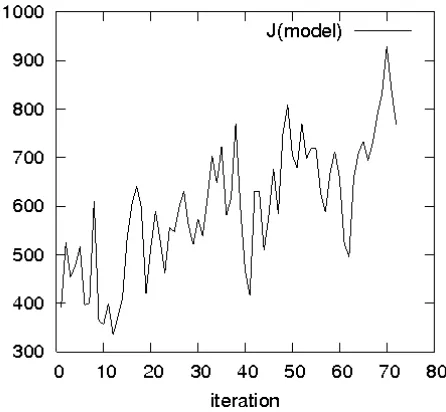
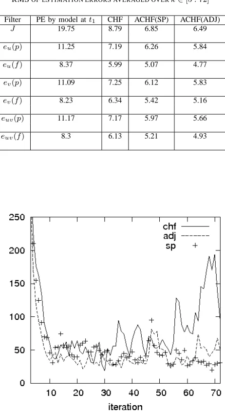
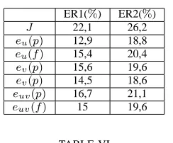
Table IV exhibits the RMS-PE and RMS of the filtered error (RMS-FE) produced by the filters CHF, ACHF(SP) and ACHF(ADJ). Here ACHF(SP) and ACHF(ADJ) denote the ACHF with the use of the SPSA or the adjoint equation method for computing the gradient vector. Mention that the ACHF(ADJ) has been studied in [4] and is presented here as reference for comparison with the ACHF(SP). From Table IV it is seen that compared to the CHF, the adaptation allows to reduce significantly the estimation error. The ACHF(ADJ), using more correct estimation of the gradient vector at the beginning of the assimilation (see below), has produced better estimates over this period. In Table V the performance improvement of two ACHFs by adaptation is displayed where the quantities ER1(%), ER2(%), expressed in percentage, show how the corresponding ACHF(SP) or ACHF(ADJ) has reduced the RMS of estimation errors compared to that of CHF. For example, over the large window k ∈ [5 : 72], the SPSA algorithm has reduced about 15 % rms errors whereas this percentage is of order 20 % if the gradient is computed by the adjoint code. Fig. 10 depicts instantaneous values of the objective function resulting from three filters. In all filters, the objective functions decrease considerably from the beginning up tok= 10. During the period k∈[10 : 30]
the errors remain more or less constant and of nearly the same level for the CHF and ACHF(SP) (about 50 cm2
). The best performance is produced by the ACHF(ADJ) with the variance of SSH innovation fluctuating around 30 cm2
. However at the final window k ∈ [30 : 72] the objective function increases significantly in the CHF.
As to two ACHFs, the mechanism of adaptation allows them to change their behaviors to respond more or less correctly to the changes in environment, hence to follow more correctly the trajectory of the true system state. If the error in the ACHF(ADJ) remains more or less of the same level as observed in the preceding window, the performance of the ACHF(SP) becomes better and better : it is capable of decreasing more and more the RMS of the innovation during all the assimilation period. This fact is clearly seen in
TABLE III
TIME AVERAGEDRMS-PEPRODUCED BYCHFANDMODELAT THE END OF ASSIMILATION PERIOD
Filter CHF MODEL
J(cm) 8.79 24.59
eu(p)(cm/s) 7.19 13.74
ev(p)(cm/s) 7.25 14.32
[image:11.612.313.544.259.683.2]euv(p)(cm/s) 7.17 14.03
TABLE IV
RMSOF ESTIMATION ERRORS AVERAGED OVERk∈[5 : 72]
Filter PE by model att1 CHF ACHF(SP) ACHF(ADJ)
J 19.75 8.79 6.85 6.49
eu(p) 11.25 7.19 6.26 5.84
eu(f) 8.37 5.99 5.07 4.77
ev(p) 11.09 7.25 6.12 5.83
ev(f) 8.23 6.34 5.42 5.16
euv(p) 11.17 7.17 5.97 5.66
euv(f) 8.3 6.13 5.21 4.93
Fig. 10. Sample objective functions resulting from three filters CHF, ACHF(SP), ACHF(ADJ).
IAENG International Journal of Applied Mathematics, 42:1, IJAM_42_1_04
TABLE V
ERROR REDUCTION(IN PERCENTAGE)ACHIEVED BYACHF(SP)AND ACHF(ADJ)
ER1(%) ER2(%) J 22,1 26,2 eu(p) 12,9 18,8
eu(f) 15,4 20,4
ev(p) 15,6 19,6
ev(p) 14,5 18,6
euv(p) 16,7 21,1
[image:12.612.86.255.208.350.2]euv(f) 15 19,6
TABLE VI
RMSOF ESTIMATION ERRORS AVERAGED OVERk∈[61 : 72]
Filter CHF ACHF(SP) ACHF(ADJ)
J 11.53 5.48 7.02
eu(p) 9.25 5.03 5.88
eu(f) 7.57 4.49 5.04
ev(p) 9.36 5.28 6.15
ev(f) 8.05 4.72 5.28
euv(p) 8.94 4.96 5.78
euv(f) 7.51 4.43 4.96
Fig. 10 with decreasing tendency of the curve ’SP’ along all assimilation period. There are two reasons for which the ACHF(SP) works better than the ACHF(ADJ) as more and more observations are assimilated. First, the ACHF(SP) approximates the gradient vector by direct difference be-tween two nonlinear integrations while the SA method uses a linearization technique. The latter introduces inevitably an additional error in gradient computation in nonlinear systems which is accumulated as the assimilation progresses. Secondly, due to simultaneous stochastic perturbation of all parameters, the SPSA naturally requires a longer assimilation time for searching a correct descent direction. That is why if the error in the gradient computation seems to be more and more important in the ACHF(ADJ) as the assimilation advances, the inverse happens in the ACHF(SP).
The effect of adaptation can be examined by looking at the assimilation results at the last four months, i.e.k∈[61 : 72], Table VI displays the RMS-PE and RMS-FE resulting from three filters. As expected, the ACHF(SP) behaves now better than the ACHF(ADJ), with the reduction of velocity error by more than 10 %. As to the CHF, during this period one observes an important increase of estimation error compared to that shown in Table IV.
C. PEF and its adaptive versions
1) PEF and its modifications: The gain of PEF (28) is
obtained by estimating the elementsωl,mofMα=0= Ω(see
Eq. (21)) from the DPE patterns (SP1). The experimental results in Table VII show that the PEF is much more efficient
Fig. 11. Variance of SSH prediction error resulting from PEF and MPEF(HORIZ) and MPEF(RIC)
TABLE VII
RMSOF ESTIMATION ERRORS AVERAGED OVERk∈[5 : 72]
Filter PEF APEF(SP) APEF(ADJ) ER1 (%) ER2 (%) J 6.36 5.90 5.88 7.2 7.5
eu(p) 5.69 5.42 5.34 4.7 6.2
eu(f) 4.77 4.48 4.45 6.1 6.7
ev(p) 5.74 5.43 5.36 5.4 6.6
ev(f) 5.10 4.83 4.79 5.3 6.1
euv(p) 5.57 5.24 5.20 5.9 6.6
euv(f) 4.90 4.62 4.59 5.7 6.3
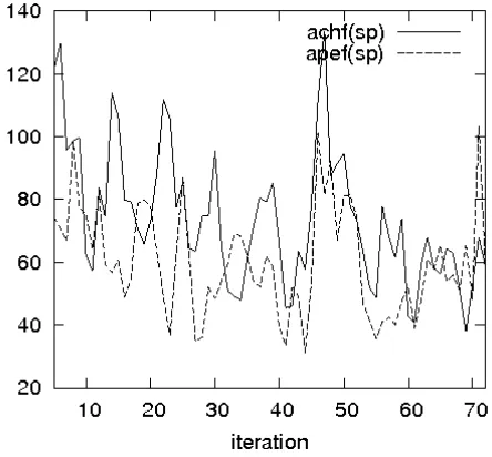
than the CHF (see Table IV) and it slightly outperforms the ACHF(SP) and ACHF(ADJ). Thus the statistics extracted from DPE samples play an important role in correct estimat-ing the filter gain and in improvestimat-ing the filter performance. To exploit the horizontal structure of the PE patterns as well as their dynamical changes during assimilation, as in the previous section, we apply two modified PEFs, namely PEF(HORIZ) and PEF(RIC). These two filters are designed in the same way as described in sections VII.A.2, VII.A.3. Assimilation results show that the similar effect is observed when adding the horizontal structure of PE in estimating the ECM or when dynamically updating the PE samples on-line using the simplified Riccati equation (see Fig. 11). For the PEF structure, the performances of two filters PEF(HORIZ) and PEF(RIC) are very similar, without a significant differ-ence as found with the CHF structure. The initial M(0)for the PEF(RIC) is taken as such resulting in the gain (28).
2) Adaptive PEF: As the errors in the PEF are much
lower than that in the CHF, there remains no great ex-pectation to reduce its errors (by adaptation) compared to the CHF case. Even though, as seen from Tables VII-VIII, the adaptation is proved to be an advantageous tool for
IAENG International Journal of Applied Mathematics, 42:1, IJAM_42_1_04
TABLE VIII
RMSOF ESTIMATION ERRORS AVERAGED OVERk∈[61 : 72]
Filter PEF APEF(SP) APEF(ADJ) ER1(%) ER2(%) J 6.94 5.75 5.96 17.1 14.1
eu(p) 5.99 5.04 5.23 15.9 12.7
eu(f) 5.26 4.44 4.59 15.6 12.7
ev(p) 6.19 5.19 5.41 16.2 12.6
ev(f) 5.47 4.56 4.82 18.5 11.9
euv(p) 5.85 4.92 5.11 15.9 12.6
[image:13.612.56.290.72.456.2]euv(f) 5.15 4.32 4.52 16.1 12.2
Fig. 12. Instantaneous RMS-PE for theu-velocity component at the 1st layer: at the final window [61:72] there is an error growth in the CHF whereas no such phenomenon is observed in the PEF.
improving the performance of the PEF. For all assimilation period, the adaptation has reduced the rms estimation error by about 5-6%in the APEF(SP) and 6-7%in the APEF(ADJ). These reductions are less important than that achieved by the ACHF(SP) and ACHF(ADJ) with respect to the CHF (they are equal to 15%and 20%respectively, see Table V). At the last 4 months, the APEF(SP) again outperforms the APEF(ADJ). Meantime, the error reduction is achieved by 16-17%in the APEF(SP) and by 12-13%in the APEF(ADJ) compared to the non-adaptive PEF.
[image:13.612.320.542.307.513.2]Finally Fig. 12 displays typical instantaneous RMS-PE for theu-velocity component at the 1st layer (the same errors are observed for other layers and for thev-component) produced by the CHF and PEF. Similarly to Fig. 10 for the SSH errors, the CHF has a difficulty to well estimate the velocity as assimilation progresses. There is a significant difference in error levels produced by the PEF and the CHF, especially at the final assimilation window [61:72].
Fig. 13. As in figure 12 but produced by ACHF(ADJ), APEF(ADJ).
Fig. 14. The same as in Fig. 12 but produced by APEF(ADJ) and APEF(SP).
It is seen from Fig 13 thanks to the PEF structure, the adaptation allows the APEF to avoid the error picks produced by the ACHF. These improvements are well summarized in Tables VII-VIII: in average, over all assimilation period, the APEF(SP) (or APEF(ADJ)) behave much better than the corresponding ACHF(SP) (or ACHF(ADJ)) and this proves that the gain of the PEF is much more close to ”optimal” than that of the CHF.
Another interesting fact, found from Fig. 13 (or Fig. 14), is that at the final window [61:72] the errors in the AFs with different gain structures (CHF or PEF) are of nearly the same level. This means that the role of the initial gain structure seems to be less important as the free parameters are gradually adjusted to minimize the PE. This effect is
IAENG International Journal of Applied Mathematics, 42:1, IJAM_42_1_04
seen more clearly by comparing the error curves in Fig. 13 with that depicted in Fig. 12 for corresponding non-adaptive filters. Here the adaptation has been applied only to the CHF and PEF. Its application to the modified filters like MCHF(HORIZ), MPEF(HORIZ) ... would lead to more efficient adaptive filters.
VIII. CONCLUSIONS
In this paper, we have demonstrated that one can get a great benefit from a proper initialization of the filter gain and its optimization by applying the SP-DPE and SPSA algorithms. Thanks to SP-DPE, the elements or parameters of the ECM are properly estimated from generated DPE samples in a low-cost way. This allows us to construct, practically in automatic way, the filter gain with appropriate parameterization. There are two simple ways to modify the structure of the filter either by exploiting the horizontal struc-ture of the PE samples or by updating the PE samples during assimilation process, taking into account the FE estimate. These modified filters are proved to be more efficient in reducing the estimation errors. More detailed investigation on how to better use the PE samples in the filter design is of importance and left for future study.
For the adaptation purpose, from the proposed gain struc-tures, the allowable intervals for the tuning parameters values can be determined. With the help of the SPSA algorithm, the optimization is performed at the cost of two integrations of the numerical model. For meteorological and oceanic models with dimension of order 107−108, this algorithm appears
to be an extremely important tool for the future development of optimal assimilation systems.
The feasibility of this approach is demonstrated in typical state and parameter estimation problems. Numerical results show that initialization of the gain using the DPE samples can yield the performance of PEF comparable with that of the KF (experiment on vehicle navigation) or allows the PEF to reduce significantly the estimation error in comparison with the traditional CHF (experiment with data assimilation in the ocean model MICOM). A significant improvement of the filter performance is demonstrated by adaptive tuning some pertinent parameters of the gain. There is no significant difference in performance between two SA algorithms, one is based on gradient estimated by AE and another - on simultaneous perturbation (SPSA). It is worthy of mention that compared to the classical SA method, the SPSA seems to be less efficient at the beginning but more efficient as more and more observations are assimilated. That is also true when SPSA is applied to optimize the filter performance for nonlinear systems. The reason is that the SPSA calculates derivatives using the difference between two nonlinear model integrations whereas the AE method approximates the gra-dient by linearization.
ACKNOWLEDGMENT
The authors would like to thank the editor and anonymous reviewers for their valuable comments and suggestions to improve the manuscript.
REFERENCES
[1] H.S. Hoang and R. Baraille, ”On an Adaptive Filter based on Simulta-neous Perturbation Stochastic Approximation Method”, Lecture Notes
in Engineering and Computer Science, V. II, WCE 2011, London,
2011, pp. 1675-1680.
[2] H.S. Hoang, P. De Mey, O. Talagrand and R. Baraille, 1997. ”A new reduced-order adaptive filter for state estimation in high dimensional systems”, Automatica. 33, pp 1475-1498., 1997.
[3] H.S. Hoang, O. Talagrand and R. Baraille, ”On the design of a stable filter for state estimation in high dimensional systems”, Automatica. 37, pp 341-359, 2001.
[4] H.S. Hoang, R. Baraille and O. Talagrand, ”On an adaptive filter for altimetric data data assimilation and its application to a primitive equation model MICOM”, Tellus, 57A, no 2, pp 153-170, 2005. [5] H.S. Hoang, O. Talagrand and R. Baraille, ”On the stability of a
reduced-order filter based on dominant singular value decomposition of the systems dynamics”, Automatica. 45, pp 2400-2405, 2009. [6] A.E. Bryson and Y.C. Ho, Applied optimal control. Washington, DC:
Hemisphere, 1975.
[7] M. Ghil, and P. Manalotte-Rizzoli, ”Data assimilation in meteorology and oceanography”, Adv. Geophys. 33, pp 141-266, 1991.
[8] H.W. Sorenson and D.L. Alspach, ”Recursive Bayesian estimation using Gaussian sums”, Automatica., 7, pp. 465479, 1971.
[9] M. S. Arulampalam, S. Maskell, N. Gordon, and T. Clapp, ”A Tu-torial on Particle Filters for Online Nonlinear/Non-Gaussian Bayesian Tracking”, IEEE Trans. Signal Proc., Vol. 50, No 2, pp 174-188, 2002. [10] R. van der Merwe, A. Doucet, N. de Freitas and E. Wan, ”The Un-scented Particle Filter”, in Advances in Neural Information Processing
Systems (NIPS13), (T. G. Dietterich T. K. Leen and V. Tresp, eds.),
2000, pp. 351357.
[11] Baili H., ”Stochastic Analysis and Particle Filtering of the Volatility”,
IAENG Int. J. Applied Math., 41:1, IJAM-41-1-09, 2009.
[12] O. Talagrand, P. Courtier, ”Variational Assimilation of Meteorological Observations with the Adjoint Vorticity Equation. Part I. Theory”, Q.
J. R. Meteorol. Soc., pp 531-549, 1987.
[13] Traore O., ”Approximate Controllability and Application to Data Assimilation Problem for a Linear Population Dynamics Model”.
IAENG Int. J. Applied Math., 37:1, IJAM-37-1-1, 2007.
[14] G. Evensen, ”The ensemble Kalman filter: Theoretical formulation and practical implementation”, Ocean Dynamics, 53, pp 343-367, 2003. [15] T.M. Hamill, ”Ensemble-based atmospheric data assimilation” In:
Predictability of Weather and Climate, Cambridge Univ. Press, pp
124-156, 2006.
[16] R. Todling and S.E. Cohn, ”Suboptimal schemes for atmospheric data assimilation based on the Kalman filter”, Mon. Wea. Rev., 122, pp 2530-2557, 1994.
[17] Y. Baram and G. Kalit, ”Order reduction in linear state estimation under performance constraints”, IEEE Trans. Autom. Contr., 32, pp 983-989, 1987.
[18] R. Fitzgerald, ”Divergence of the Kalman filter”, IEEE Trans. Autom.
Contr., 16, pp 736-747, 1971.
[19] S.E. Cohn and R. Todling, ”Approximate data assimilation schemes for stable and unstable dynamics”, Journal of Meteorological Society
of Japan, 97, pp 9479-9492, 1992.
[20] M. Cooper and K. Haines, ”Altimetric assimilation with water property conservation”, J. Geophys. Res., 101, 1059-1077, 1996.
[21] H.S. Hoang and R. Baraille, ”Prediction error sampling procedure based on dominant Schur decomposition. Application to state estima-tion in high dimensional oceanic model”, Appl. Math. Comput., 218, pp. 3689-3709, 2011.
[22] T. Kailath, ”An Innovations Approach to Least-Squares Estimation, Pt. I: Linear Filtering in Additive Noise”, IEEE Trans. Autom. Contr., December, pp. 646-655, 1968.
[23] Y. Halevi, ”The optimal reduced-order estimator for systems with singular measurement noise”, IEEE Trans. Autom. Contr., 34, pp 777-783, 1989.
[24] G.H. Golub and C.F. Van Loan, Matrix Computations, 2 edn. Johns Hopkins, 1993.
[25] Ya. Zypkin, Adaptation and Learning in Automatic Systems, New York, Academic, 1971.
[26] C.S. Spall, ”An Overview of the Simultaneous Perturbation Method for Efficient Optimization”, Johns Hopkins Apl Tech. Digest, V. 19, No 4, 482-492, 1998.
IAENG International Journal of Applied Mathematics, 42:1, IJAM_42_1_04
[27] D. Simon, ”Kalman Filtering”, in Embedded Systems Programming, June, pp 72-79, 2001.
Hong Son Hoang M’11 received the MSc degree in Applied Mathematics
from Belorussian State University, Minsk (in former USSR) in 1977 and the Doctorate degree from Hanoi Polytechnical Institute in 1988. He is presently Research Engineer on applied mathematics at the Service Hydrographique et Oc´eanographique de la Marine (SHOM/CMO) Toulouse, France. His research interests are in general area of adaptive estimation and control, stochastic stability and inverse problems of mathematical physics. Currently he is concentrated on adaptive filtering for uncertain distributed parameter systems and the theory of optimal perturbations with application to data assimilation in oceanography.
R´emy Baraille obtained the Doctorate degree in Applied Mathematics from
Bordeaux University I, Bourdeaux, France in 1991. Since 1992, he has been Research Engineer at the Service Hydrographique et Oc´eanographique de la Marine, Touloue, France. His research interests lie in numerical methods for hyperbolic partial differential equations, oceanographic modeling, and data assimilation.