Fuzzy Modeling using Neural Gas
Hirofumi Miyajima, Noritaka Shigei, Hiromi Miyajima
Abstract—Fuzzy modeling has been extensively studied. Among them, it has been shown that fuzzy modeling methods using vector quantization (VQ) and steepest descent method (SDM) are effective in terms of the number of rules (parame-ters). The methods firstly determine the initial parameter values of fuzzy rules by using VQ with learning data, and then tune the parameters by using SDM. On the other hand, Neural Gas (NG) is known as a novel approach of VQ and NG with local linear mappings (LLMs) has been applied to a time-series prediction problem. In the application, the predicted value in each of subregions is approximated by using a corresponding linear mapping. It has been demonstrated that, compared with K-means with RBF, NG with LLMs is advantageous in terms of the accuracy and the number of subregions. The idea of NG with LLMs has been applied to fuzzy modeling with TS fuzzy model, and its effectiveness has been demonstrated. However, the effectiveness of this approach has not been been confirmed for simpler fuzzy model such as simplified fuzzy model. This paper proposes to apply the concept of NG with LLMs to fuzzy modeling with simplified fuzzy inference model. The proposed method firstly determines the initial parameter values of fuzzy rules including the weights in the consequent part by using NG and supervised learning, and then tunes the parameters by using SDM. The effectiveness of the proposed method with sim-plified fuzzy modeling is demonstrated in numerical simulations of function approximation and classification problems.
Index Terms—Simplified Fuzzy Inference Model, Vector Quantization, Neural Gas, Local Linear Mapping
I. INTRODUCTION
W
ITH increasing interest in Artificial Intelligence (AI), extensive studies related to Machine Learning (ML) have been done. In the field of ML, supervised learning such as backpropagation, unsupervised one such as K-means, and Reinforcement Learning (RL) are well known. ML for fuzzy inference models, called fuzzy modeling, is one of the supervised ones, and extensive studies on fuzzy modeling have also been made [1], [2]. Although most of fuzzy modeling methods are based on steepest descent method (SDM), their obvious drawbacks are its large time complexity, getting stuck easily in shallow local minima and difficulty of applying to high dimensional data. In order to overcome the drawbacks, the followings have been developed: 1) creating fuzzy rules one by one starting from a few rules, or deleting fuzzy rules one by one starting from many rules [3], 2) using evolutionary algorithms such as GA and PSO to determine parameters of fuzzy inference systems [4], 3) fuzzy inference systems composed of rule modules with a few inputs such as SIRMs (Single Input Rule Modules) and DIRMs (Double Input Rule Modules) methods [5], and 4) determining the initial assignment of learning parameters by using self-organization map (SOM) or VQ [6], [7]. Especially, with fuzzy modeling using VQHirofumi Miyajima is Faculty of Informatics, Okayama University of Science, Japan e-mail: [email protected]
Noritaka Shigei is with Kagoshima University. Hiromi Miyajima is with Former Kagoshima University.
methods such as K-means, Neural-Gas (NG), SOM and fuzzy c-means, there are many studies on how to realize the system with high accuracy and a few rules [8], [9]. The methods firstly determine the initial parameter values of the antecedent part of rules by VQ using only input or both input and output information of learning data, and then tune the parameters by using SDM. Further, in addition to initial assignments of the antecedent part, it also has been proposed to determine the initial assignments of weight parameters of the consequent part by using VQ [8], [9].
Neural Gas (NG) is known as a novel approach of VQ and NG with local linear mappings (LLMs) has been applied to a time-series prediction problem [10]. In the application, the predicted value in each of subregions is approximated by us-ing a correspondus-ing linear mappus-ing. It has been demonstrated that, compared with K-means with RBF, NG with LLMs is advantageous in terms of the number of subregions, each of which is approximated by using a linear mapping. The similar idea has been applied to fuzzy modeling with TS fuzzy model, and its effectiveness has been demonstrated [11]. However, the effectiveness of the similar approach has not been been confirmed for simpler fuzzy model such as simplified
This paper proposes to apply the concept of NG with LLMs to fuzzy modeling with simplified fuzzy inference model. Before tuning the parameters by using SDM, the proposed method determines the initial parameter values of fuzzy rules including the weights in the consequent part by using NG and supervised learning. The determination of the initial parameter values of the consequent part firstly divides the input space into Voronoi subregions, and then determines a constant value well approximating the output value of each subregion by using supervised learning. The effectiveness of the proposed method with simplified fuzzy modeling is demonstrated in numerical simulations of func-tion approximafunc-tion and classificafunc-tion problems. In Secfunc-tion II, conventional learning methods of fuzzy model, NG and NG with supervised learning are introduced. In Section III, a learning method for the simplified fuzzy model using NG is proposed. In Section IV, numerical simulations for function approximation and classification problems are performed to demonstrate the effectiveness of the proposed method.
II. PRELIMINARIES
A. The simplified fuzzy inference models
The conventional (simplified) fuzzy inference model using SDM is described [1]. Let Zj = {1,· · ·, j} and Zj∗ =
{0,1,· · ·, j}for the positive integerj. LetRbe the set of real numbers. Letx= (x1,· · ·, xm)andyr be input and output data, respectively, wherexi∈R fori∈Zmandyr∈R. Then the rule of fuzzy inference model is expressed as
Ri : if x1 isMi1 and· · ·xj isMij· · · andxmis Mim
wherei ∈ Zn is a rule number, j is a variable number, Mij is a membership function of the antecedent part, andwi is the weight of the consequent part.
A membership valueµiof the antecedent part for inputx
is expressed as
µi= m
∏
j=1
Mij(xj). (2)
The outputy∗ of fuzzy inference is obtained as follows:
y∗=
∑n i=1µiwi
∑n i=1µi
(3)
If Gaussian membership function is used, then Mij is expressed as follow:
Mij(xj) = exp
(
−1
2
(
xj−cij bij
)2)
(4)
wherecij andbij denote the center and the width values of Mij, respectively.
In order to realize the effective model, conventional learn-ing is introduced.
Let D = {(xp1,· · ·, xp
m, ypr)|p ∈ ZP} be the set of learning data. The objective of learning is to minimize the following mean square error (MSE). The objective function E is determined to evaluate the inference error between the desirable output yrand the inference output y∗ as follows :
E = 1 P
P
∑
p=1
(y∗p−yrp)2. (5)
In order to minimize the objective function E, each parameter α ∈ {cij, bij, wi} is updated based on SDM (Steepest Descent Method) as follows [1]:
α(t+ 1) =α(t)−Kα ∂E
∂α (6)
where t is iteration time and Kα is a constant. When the Gaussian membership function is used as the membership function, the following relation holds.
∂E ∂wi =
µi
∑n i=1µi
(y∗−yr) (7)
∂E ∂cij =
µi
∑n i=1µi
(y∗−yr)(wi−y∗) xj−cij
b2ij (8)
∂E ∂bij =
µi
∑n i=1µi
(y∗−yr)(wi−y∗)
(xj−cij)2 b3
ij
(9)
wherei∈Zn andj∈Zm.
The conventional learning algorithm is shown as follows [1], where θ andTmax are the threshold and the maximum number of learning, respectively. Note that the method is a generative one, which creates fuzzy rules one by one starting from any number of rules. The method is called learning algorithm A.
Learning Algorithm A
Input : Learning data D={(xp1,· · ·, xp
m, ypr)|p∈ZP} Output : Parameters c,bandw
Step A1 : The initial number n of rules is set to n0. Let t= 1.
Step A2 : The parameterscij,bij andwiare set randomly.
Step A3 : Letp= 1.
Step A4 : A data(xp1,· · ·, xpm, ypr)∈D is given.
Step A5 : From Eqs.(2) and (3),µi andy∗ are computed, respectively.
Step A6 : Parameterswi,cijandbij are updated by Eqs.(7), (8) and (9), respectively.
Step A7 : Ifp=P, then go to Step A8 and ifp < P, then go to Step A4 withp←p+ 1.
Step A8 : Let E(t)be inference error at step t calculated by Eq.(5). If E(t)> θ and t < Tmax, then go to Step A3 witht←t+ 1else ifE(t)≤θ, then the algorithm terminates.
Step A9 : If t > Tmax andE(t)> θ, then go to Step A2 withn←n+ 1andt= 1.
B. Neural gas and K-means
Vector quantization techniques encode a data space, e.g., a subspaceV⊆Rd, utilizing only a finite setU ={u
i|i∈Zr} of reference vectors (also called cluster centers), wheredand rare positive integers.
Let the winner vectorui(v)be defined for any vectorv∈V as follows:
i(v) = arg min i∈Zr
||v−ui|| (10)
From the finite setU,V is partitioned as follows:
Vi={v∈V|||v−ui||≤||v−uj|| f or j∈Zr} (11)
For NG [10], the following method is used:
Given an input data vector v, we determine the neighborhood-rankinguik for k∈Zr∗−1, being the reference vector for which there arek vectorsuj with
||v−uj||<||v−uik|| (12)
If we denote the numberkassociated with each vectorui byki(v,ui), then the adaption step for adjusting theui’s is given by
△ui = εhλ(ki(v,ui))(v−ui) (13) hλ(ki(v,ui)) = exp (−ki(v,ui)/λ)) (14)
ε = εint
(
εf in εint
) t
Tmax
where ε∈[0,1] and λ > 0. The number λ is called decay constant.
The evaluation function for the partition is defined as follows:
E= ∑
ui∈U
∑
v∈V
hλ(ki(v,ui))
∑
ul∈Uhλ(kl(v,ul))
||v−ui(v)||2 (15)
Ifλ→0, Eq.(13) becomes equivalent to the K-means [10]. Otherwise, not only the winnerui0 but the second, third
nearest reference vector ui1, ui2, · · · are also updated in
learning.
Let D∗ = {xp|p∈ZP} for the set D. Let p(v) be the probability distribution forv∈V. Then, NG is introduced as follows [10]:
Learning Algorithm B∗ (Neural Gas)
Input : The setV of data
Output : The setU of reference vectors
Step B∗2 : Let t= 1.
Step B∗3 : Give a data v∈V based on p(x) and neighborhood-rankingki(v,ui)is determined.
Step B∗4 : Each reference vector ui for i∈Zr is updated based on Eq.(13)
Step B∗5 : If t≥Tmax, then the algorithm terminates and the set U = {ui|i∈Zr} of reference vectors is obtained. Otherwise go to Step B∗3 ast←t+ 1.
If the data distribution p(v) is not given in advance, a stochastic sequence of input data v(1),v(2),· · · which is based on p(v)is given.
By using Learning Algorithm B∗, the learning method of the fuzzy system is introduced as follows [8]. In this case, assume that the distribution of the setD∗ of learning data is a discrete uniform one. Letn0be the initial number of rules andn=n0.
Learning Algorithm B (Learning of fuzzy inference system using NG)
Input : Learning data D∗={(xp1,· · ·, xp
m)|p∈ZP} Output : Parameters c,bandw
Step B1 : For learning data D∗, Learning Algorithm B∗ is performed and the setU of reference vectors is obtained, where|U|=n.
Step B2 : Each element of the set U is set to the center parametercof each fuzzy rule. Further, the width parameter bij is set as follows :
bij= 1 mi
∑
xk∈Ci
(cij−xkj)2, (16)
where Ci and mi are the set of learning data belonging to the i-th cluster and its cardinal number, respectively. Each initial value ofwi is selected randomly. Lett= 1.
Step B3 : The Steps A3 to A8 of learning algorithm A are performed.
Step B4 : If t≥Tmax and E(t) > θ, then go to Step B1 withn←n+ 1.
C. Adaptive local linear mapping
In this section, the learning method to adaptively approx-imate the function y = f(v) with v∈V⊆Rd and y∈R using NG is introduced based on Ref. [10]. The set V denotes the function’s domain. Let n be the number of computational units, each containing a reference vector ui together with a constant ai0 and d-dimensional vectors ai. Learning Algorithm B∗ assigns each unitito a subregionVi as defined in Eq.(11), and the coefficientsai0 andai define a linear mapping
g(v) =ai0+ai(v−ui) (17)
fromRd toRover each of the Voronoi diagramVi. Hence, the function y=f(v)is approximated byy˜=g(v)with
g(v) =ai(v)0+ai(v)(v−ui(v)) (18)
wherei(v)denotes uniti with itsui closest tov.
To learn the input-output mapping, a series of learning steps by approximatingD={(xp, ypr)|p∈ZP}is performed. In order to obtain the output coefficients ai0 and ai, the mean squared error |V1|∑v∈V (f(v)−g(v))2 between the desirable and the obtained output, averaged over subregion
Vi, to be minimal is required for each i. Gradient descent with respect toai0 andai yields [10].
△ai0 = ε′hλ′(ki(v,ui))(y−ai0−ai(v−ui)) (19)
△ai = ε′hλ′(ki(v,ui))(y−ai0−ai(v−ui))(v−ui) (20)
whereε′ >0andλ′>0.
In order to apply the method with adaptively local linear mapping (LLM) to fuzzy modeling of the simplified fuzzy system, all parameters ai’s are not used. That is, the con-stantsai0’s only are updated.
The algorithm is introduced as follows :
Learning Algorithm C
Input : Learning data D = {(xp, y
p)|p∈ZP} and D∗ =
{xp|p∈Z P}.
Output : The setU of reference vectors and the coefficient ai0 fori∈Zn.
Step C1 : The set U of reference vectors is determined using D∗ by Algorithm B∗. The subregionsVi for i∈Zn is determined usingU, whereVi is defined by Eq.(11), Vd =
∪n
i=1Vi andVi∩Vj=∅ (i̸=j).
Step C2 : Each parameter ai0(i∈Zn)is set randomly. Let t= 1.
Step C3 : A learning data (x, y)∈D is selected based on p(x). The rankki(x,ui)of xfor the setVi is determined.
Step C4 : Each parameter ai0 for i∈Zn is updated based on the following Eq.(21).
ai0(t+ 1) =ai0(t) +ε′hλ(ki(v,ui))(y−ai0) (21)
Step C5 : Ift≥Tmax, then the algorithm terminates else go to Step C3 witht←t+ 1, whereTmaxmeans the maximum number of learning times.
Remark that Algorithm C is one of the learning methods using NG and SDM [10]. Likewise, the learning methods us-ing other VQ such as k-means and SDM are also considered.
D. The appearance probability of learning data based on the rate of change of output
Learning Algorithm B is a method that determines the initial assignment of fuzzy rules by vector quantization using the set D∗. In the previous paper, we proposed a method using both input and output parts of D to determine the initial assignment of parameters of the antecedent part of fuzzy rule [8].
Based on Ref. [8], the appearance probability is defined as follows :
Algorithm for Appearance Probability (Algorithm AP)
Input : Learning data D={(xp1,· · ·, xp
m, ypr)|p∈ZP} and
D∗={(xp1,· · ·, xp
m)|p∈ZP}
Output : Appearance probabilitypM(x)forx∈D∗
Step 1 : Give an input data xi∈D∗, we determine the neighborhood-ranking (xi0,xi1,· · ·,xik,· · ·,xiP−1) of the
vector xi with xi0 = xi, xi1 being closest to xi and xik(k = 0,· · ·, P −1) being the vector xi for which there
arek vectorsxj with||xi−xj||<||xi−xik||.
xi, by the following equation:
H(xi) = M
∑
l=1
|yi−yil|
||xi−xil|| (22)
where xil for l∈Z
M means the l-th neighborhood-ranking of xi,i∈Z
P andyi andyil are output for input xi andxil, respectively. The number M means the range considering H(x).
Step 3 : Determine the appearance probabilitypM(xi)for
xi by normalizing H(xi).
pM(xi) = H(x i)
∑P
j=1H(xj)
(23)
The method is called Algorithm AP.
Learning algorithm F using Algorithm AP to fuzzy mod-eling is obtained as follows:
Learning Algorithm F
Input : Learning data D={(xp1,· · ·, xp
m, yrp)|p∈ZP} and
D∗={(xp1,· · ·, xp
m)|p∈ZP} Output : Parameters c,bandw.
Step F1 : The constantsθ,T0
max,TmaxandM0for 1≤M0 are set. Let M =M0. The probabilitypM(x)for x∈D∗ is computed using Algorithm AP. The initial numbernof rules is set.
Step F2 : The initial values of cij, bij and wi are set randomly. Let t= 1.
Step F3 : Select a datax∈D∗ based on pM(x).
Step F4 : Updatecij by Eq.(14) to approximate the setD∗ by the set of center parameters cij’s of fuzzy rule.
Step F5 : If t < T0
max, go to Step F3 with t←t + 1, otherwise go to Step F6 witht←1.
Step F6 : Determinebij by Eq.(16).
Step F7 : Letp= 1.
Step F8 : Given data(xp, yr p)∈D.
Step F9 : Calculateµi andy∗ by Eqs.(2) and (4).
Step F10 : Update parameterswi, cij andbij by Eqs.(7), (8) and (9).
Step F11 : Ifp < P then go to Step F8 withp←p+ 1.
Step F12 : If E > θ and t < Tmax then go to Step F8 witht←t+ 1, whereE is computed as Eq.(5), and ifE < θ then the algorithm terminate, otherwise go to Step F2 with n←n+ 1.
In Algorithm F, the SDM processes of F7 to F12 are performed after the initial values of parameters c and bof F4 to F6 are set.
As shown in Ref. [8], learning algorithm F realizes that many rules are needed at or near the places where output changes rapidly in learning data. The probability pM(x) is one method to perform it [8]. See the Ref. [8] about the detailed explanation of Algorithms AP and F for the simplified fuzzy modeling.
III. THEPROPOSED FUZZY MODELING USINGNG
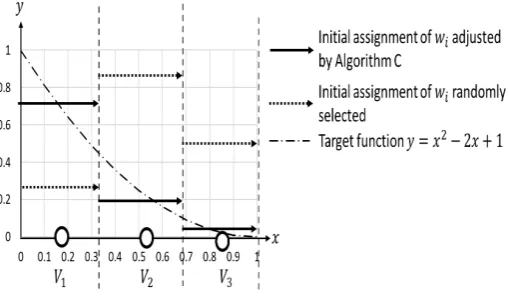
[image:4.595.308.563.57.205.2]It is known that the assignment of the initial parameters by VQ can improve the performance of fuzzy modeling based on SDM in terms of accuracy and the number of rules. For TS fuzzy inference model, which is superior to the simplified fuzzy inference model in terms of accuracy, it has been
Fig. 1. The figure to explain an Example.
already proposed to assign the initial values of the weight parameters in the consequent part of fuzzy rules by using NG and its effectiveness has been demonstrated [11]. However, for simplified fuzzy inference model, a similar approach has not been proposed, and most of the conventional initialization methods using VQ take into account only the parameters of the antecedent parts of fuzzy rules. Therefore, for simplified fuzzy inference model, a new learning method using the Learning Algorithm C is proposed as follows:
Learning Algorithm G
Input : Learning data D = {(xp, yp)| p∈ZP} and D∗ =
{xp|p∈ZP}.
Output : Parametersc,bandw.
Step G1 : Letθ,Tmax1,Tmax2andTmax3be the threshold of inference error, the maximum numbers of learning time for NG and the maximum number of learning time for SDM, respectively.
Step G2 : From Algorithm AP, the probability pM(x) is computed using the setD of learning data.
Step G3 : From Algorithm B∗, the setUof reference vectors is computed usingpM(x).
Step G4 : From Algorithm C, parametersai0’s of LLM are computed using the setU.
Step G5 : Each element of the set U is set to the center parametercof each fuzzy rule and the widthbof each fuzzy rule is computed from Eq.(16). Each parameterai0of LLM is set to the initial weightwi of fuzzy rule. Let t= 1.
Step G6 : Steps A3 to A7 of Algorithm A are performed forc,bandw.
Step G7 : Inference error E(t) of Eq.(5) is calculated. If E(t)≤θ or t=Tmax3 then go to Step G8. If E(t)> θ and t < Tmax3, then go to Step G6 witht←t+ 1.
Step G8 : If E(t)≤θ, then the algorithm terminates. If E(t)> θ, then go to Step G3 withn←n+ 1.
In Algorithm G, initial values of parameterscandbusing G2 and G3, and parameters w using G4 are considered, respectively. Further, the SDM processes of steps G5 to G7 are performed.
Let us explain Algorithm G using an example. [Example]
TABLE I
THE APPEARANCE PROBABILITYp3(x)FOREXAMPLE OF
y=x2−2x+ 1
{0.1×k|k∈Z10∗ } andD={(x, x2−2x+ 1)|x∈D∗}. From Steps G1 and G2, a probabilitypM(x)is computed as shown in Table I, where the numberrof reference vectors is 3. From Step G3, NG is performed based on pM(x). Let M = 3. For example, two reference vectors are assigned in the interval from 0 to 0.7, and one reference vector is assigned for the remaining interval. Three regionsV1,V2and V3 shown in Fig.1 are defined as Voronoi regions from the set U of reference vectors. From Step G4, a linear function is defined in each region. In the example, interval linear functions (constants) as shown in Fig.1 are obtained as the result of Algorithm C. If Algorithm C is not used, each linear function (constant) is given randomly as shown in Fig.1. From Step G5, the initial parameters of fuzzy rules are determined, respectively.
At Step G6, the conventional SDM is performed and parameters c, b and w are updated. If sufficient accuracy cannot be obtained, a fuzzy rule is adaptively added at Step G8.
IV. NUMERICAL SIMULATIONS
In order to show the effectiveness of the proposed method, numerical simulations of function approximation and classi-fication problems.
A. The conventional and proposed methods
In the following, the conventional algorithms are (a), (b), (c) and (d) and the proposed algorithm is (c’). (a), (b), (c) and (c’) are for simplified fuzzy inference model and (d) for TS fuzzy inference model.
(a) The method (a) is Learning Algorithm A, which is the primitive learning method for the simplified fuzzy system [1]. Initial parameters of the system are set randomly and all parameters are updated using SDM until the inference error becomes sufficiently small.
(b) The method (b) is generalized one of learning method of RBF network [1]. The initial values of center parameters are determined using learning dataD∗by NG and the width parameters are computed using the center parameters from Eq.16 [8]. The initial parameters of the weight are randomly selected. Further, all parameters are updated using SDM until the inference error becomes sufficiently small (See Fig.2(b)). (c) The method (c) is Learning Algorithm F. Initial param-eters of the center are determined using learning data D by NG and the initial parameters of the width are computed using the center parameters from Eq.16 [8]. The initial as-signment of weight parameters is randomly selected. Further, all parameters are updated using SDM until the inference error becomes sufficiently small.
[image:5.595.326.551.541.666.2](c’) The method (c’) is Learning Algorithm G. In addition to the initial assignment of the method (c), the initial assignment
Fig. 2. Four charts of conventional and proposed algorithms : SDM and NG mean Steepest Descent Method and Neural Gas. The feedback loop (the under arrow) means adding of a fuzzy rule, where D = {(xp1,· · ·, xpm, yrp)|p∈ZP}andD∗={(xp1,· · ·, x
p
m)|p∈ZP}.
of weight parameters of the consequent part is determined by Learning Algorithm C. Further, all parameters are updated using SDM until the inference error becomes sufficiently small (See Fig.2(c’)).
(d) The method (d) is Algorithm E in Ref. [11] and is the version of TS fuzzy model of (c’). The simulation results are presented only for pattern classification problems.
B. Function approximation
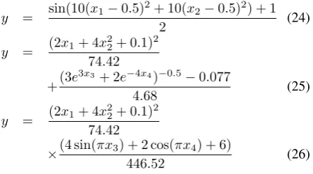
The systems are identified by fuzzy inference systems. This simulation uses three systems specified by the following functions with 2 and 4-dimensional input space [0,1]2 for Eq.(24) and[−1,1]4for Eqs.(25) and (26), respectively, and one output with the range [0,1]. The numbers of Learning and Test data are 1000 and 1000 selected from the uniform random numbers, respectively.
y = sin(10(x1−0.5)
2+ 10(x
2−0.5)2) + 1
2 (24)
y = (2x1+ 4x 2 2+ 0.1)2 74.42
+(3e
3x3+ 2e−4x4)−0.5−0.077
4.68 (25)
y = (2x1+ 4x 2 2+ 0.1)2 74.42
×(4 sin(πx3) + 2 cos(πx4) + 6)
446.52 (26)
The constantsθ,Tmax,Kcij,Kbij andKwi for each algo-rithm are1.0×10−4,50000,0.01,0.01and0.1, respectively. The constantsεinit,εf inandλfor methods (b), (c) and (c’) are0.1,0.01and0.7, respectively. The constantsε′init,ε′f in and λ′ for method (c’) are 0.1, 0.01 and 0.7, respectively. On methods (c) and (c’), the numberM for the probability pM(x) is 500 for Eqs.(24) and (26) and 300 for Eq.(25), respectively.
TABLE II
THE RESULT FOR FUNCTION APPROXIMATION
Method Eq.(24) Eq.(25) Eq.(26)
the number of rules 5.00 11.60 6.20 (a) MSE for Learning(×10−4) 0.34 0.07 0.03
MSE of Test(×10−4) 0.35 0.48 0.44
the number of rules 3.90 8.55 4.80 (b) MSE of Learning(×10−4) 0.23 0.07 0.03
MSE of Test(×10−4) 0.27 0.09 0.03
the number of rules 3.75 7.75 4.65 (c) MSE of Learning(×10−4) 0.22 0.07 0.03
MSE of Test(×10−4) 0.23 0.08 0.03
the number of rules 3.50 7.60 4.70 (c’) MSE of Learning(×10−4) 0.26 0.07 0.03
MSE of Test(×10−4) 0.27 0.09 0.03
the thresholdθ= 1.0×10⁻⁴of inference error is achieved in learning. The result of simulation is the average value from twenty trials. As a result, proposed method (c’) reduces the number of rules compared to conventional methods while keeping the accuracy.
C. Classification problems
Iris, Wine, BCW and Sonar data from the UCI database are used for numerical simulation [12]. The numbers of data are 150, 178, 683 and 208, the numbers of input are 4, 13, 9 and 60 and the numbers of classes are 3, 3, 2 and 2, respectively. In this simulation, 5-fold cross-validation is used as the evaluation method. Threshold θ is0.01 on Iris, 0.001 on Wine and 0.02 on BCW and Sonar, respectively. The constants Tmax, Kcij, Kbij and Kwi for each method
are 50000, 0.01, 0.01 and 0.1, respectively. The constants εinit,εf inandλfor methods (b), (c), and (c’) are 0.1,0.01 and 0.7, respectively. The constants ε′init, ε′f in and λ′ for methods (c’) and (d) are 0.1,0.01and0.7, respectively. On methods (c), (c’) and (d), the numberM for the probability pM(x)is 100 for Iris, Wine and Sonar and 200 for BCW, respectively.
Table III shows the result of classification for each method, where the number of rules means one when the thresholdθ of inference error is achieved in learning. In Table III, the number of rules and RM’s for learning and test are shown, where RM means the rate of misclassification. The result of simulation is the average value from twenty trials. It is shown that, among all the results, the proposed method (c’) achieves the best or comparable performance in terms of both of accuracy of the number of rules. It should be noted that the proposed method (c’) outperforms the conventional method (d) using TS fuzzy model for most cases.
V. CONCLUSION
In this paper, a new learning method of fuzzy modeling using NG with supervised learning (LLM) was proposed for simplified fuzzy inference model. Conventional learning methods using NG are to perform initial assignment only for antecedent part of fuzzy rules. In order to assign the initial values of weight parameters in the consequent part of fuzzy rules, the proposed method firstly dividing the input space into Voronoi subregion by using NG and then assign a constant to each subregion by using supervised learning (LLM). The simulation results on function approximation and pattern classification show that the proposed method
TABLE III
THE RESULT FOR PATTERN CLASSIFICATION
Method Iris Wine BCW Sonar
the number of rules 2.34 4.14 2.60 7.11 (a) RM for Learning(%) 3.54 0.27 2.21 0.99 RM of Test(%) 4.90 4.47 3.67 18.07 the number of rules 2.15 3.34 2.36 4.91 (b) RM of Learning(%) 3.42 0.30 2.23 0.67 RM of Test(%) 4.40 3.33 3.66 17.26 the number of rules 2.10 3.26 2.05 2.61 (c) RM of Learning(%) 3.48 0.26 2.19 1.73 RM of Test(%) 4.50 3.31 3.43 17.12 the number of rules 2.00 3.00 2.00 2.41 (c’) RM of Learning(%) 3.50 0.35 2.19 1.81 RM of Test(%) 4.60 3.14 3.41 16.20 the number of rules 2.0 2.0 2.0 2.8 (d) RM of Learning(%) 2.57 1.46 2.46 0.14
RM of Test(%) 4.33 4.42 3.87 23.45
achieves the best or comparable performance in terms of both of accuracy and the number of rules. Notably, the simulation results of pattern classification show that the proposed method for simplified fuzzy model is more effective than the similar approach for TS fuzzy model. From the result, it is considered that simpler model is suitable for this approach. Further, the proposed method is also superior to the method using generalized inverse matrix to determine the initial assignment of weight parameters [13]. In future work, further improvement of fuzzy modeling using VQ will be considered and applied to other problems.
REFERENCES
[1] M.M. Gupta, L. Jin and N. Homma, Static and Dynamic Neural Networks, IEEE Press, 2003.
[2] J. Casillas, O. Cordon, F. Herrera and L. Magdalena, Accuracy Im-provements in Linguistic Fuzzy Modeling, Studies in Fuzziness and Soft Computing, Vol. 129, Springer, 2003.
[3] S. Fukumoto, H. Miyajima, K. Kishida and Y. Nagasawa, A Destructive Learning Method of Fuzzy Inference Rules, Proc. of IEEE on Fuzzy Systems, pp.687-694, 1995.
[4] O. Cordon, A historical review of evolutionary learning methods for Mamdani-type fuzzy rule-based systems, Designing interpretable genetic fuzzy systems, Journal of Approximate Reasoning, 52, pp.894-913, 2011.
[5] H. Miyajima, N. Shigei and H. Miyajima, Fuzzy Inference Systems Composed of Double-Input Rule Modules for Obstacle Avoidance Problems, IAENG International Journal of Computer Science, Vol. 41, Issue 4, pp.222-230, 2014.
[6] K. Kishida and H. Miyajima, A Learning Method of Fuzzy Inference Rules using Vector Quantization, Proc. of the Int. Conf. on Artificial Neural Networks, Vol.2, pp.827-832, 1998.
[7] S. Fukumoto, H. Miyajima, N. Shigei and K. Uchikoba, A Decision Procedure of the Initial Values of Fuzzy Inference System Using Counterpropagation Networks, Journal of Signal Processing, Vol.9, No.4, pp.335-342, 2005.
[8] H. Miyajima, N. Shigei and H. Miyajima, Fuzzy Modeling using Vector Quantization based on Input and Output Learning Data, International MultiConference of Engineers and Computer Scientists 2017, Vol.I, pp.1-6, Hong Kong, March, 2017.
[9] W. Pedrycz, H. Izakian, Cluster-Centric Fuzzy Modeling, IEEE Trans. on Fuzzy Systems, Vol. 22, Issue 6, pp. 1585-1597, 2014.
[10] T. M. Martinetz, S. G. Berkovich and K. J. Schulten, Neural Gas Network for Vector Quantization and its Application to Time-series Prediction, IEEE Trans. Neural Network, 4, 4, pp.558-569, 1993. [11] H. Miyajima, N. Shigei and H. Miyajima, Fuzzy Modeling using
Vector Quantization with Supervised Learning, International MultiCon-ference of Engineers and Computer Scientists 2018, Vol.I, pp.17-22, Hong Kong, March, 2018.
[12] UCI Repository of Machine Learning Databases:,https://archive.ics.uci.edu/ml/index.php (Mar.20.2019). [13] H. Miyajima, N. Shigei and H. Miyajima, Learning Algorithms for