A Bayesian Approach to Inference and Prediction
for Spatially Correlated Count Data Based on
Gaussian Copula Model
Yan Fang
Abstract—Gaussian Copula has been successfully applied in spatially correlated count data due to its ability to completely model the high-dimensional dependence. In this article, we develop a Bayesian method to fulfill both parameter estima-tion and spatial predicestima-tion for spatially correlated count data set. A MCMC scheme (MetropolisCHastings Algorithm plus rejection sampling) is adopted to iteratively update parameter estimates; upon convergence the parameters are then used for spatial (missing count data) prediction. In terms of parameter estimation, we show that our approach yields better and more consistent results than the existing method and that our approach can significantly decrease computational burden, in the same real-life data set. Moreover, we compare the spatial prediction performance to the common Generalized Additive Models (GAM). The results in the real-life dataset as well as a well-designed simulated data set both demonstrate that our approach outperforms GAMs, especially when the missing data is small.
Index Terms—geostatistical, Gaussian copula, effective range, spatially correlated, count data, Bayesian inference, soil science, MCMC.
I. INTRODUCTION
S
PATIALLY correlated count data arise in many situation-s, such as in agriculture, ecology, and so on. However, when modeling this kind of data, people often face some technical issues related to non-Gaussian distribution and to over-dispersion. In addition, the introduction of spatial dependence in count variable may cause greatly complicates in estimation and specification testing, thus spatial model-s for dependent count variablemodel-s are model-still quite imperfect. Nevertheless, the studies focusing on spatial models for count variables and developing appropriate methods for their estimation and prediction have attracted more and more attention recently (e.g., LeSage [19]; Gschl¨oßl and Czado [16]).Accurate parameter estimation is crucial for making rea-sonable predictions when working with spatially correlated data. Traditional geostatistical methods (see, e.g., Cressie [5]) are based on normality assumption, which is not valid for discrete data. Liang and Zeger [20] and Zeger and Liang [28] introduced generalized estimating equation (GEE) to estimate unknown parameters for a discrete response variable. Howev-er, GEE is unsatisfactory for spatially correlated count data,
Manuscript received Feb. 23, 2014; revised May 20, 2014. This work was supported by Shanghai University of International Business and Economics under Grant YC-XK-13108 and under 085 Leading Academic Discipline Project. This paper is also funded by the Shanghai Pujiang Talent Plan (14PJ1404100) and the National Natural Science Foundation of China (71203139).
Y. Fang is affliated to School of Finance, Shanghai University of International Business and Economics, Shanghai, 201620, China. E-mail: [email protected].
since it contains n-fold summation in the model. In order to avoid n-fold summation in GEE, more recently, Madsen [21] proposed a maximum likelihood method (hereafter referred to as MML) to estimate the unknown parameters, where dependent count data are brought into the geostatistical framework by means of Gaussian copula (its application of Gaussian copula, please refer to Song et al. [26], Fang and Madsen [12], Fang et al. [13], and so on). Since the Gaussian copula makes no assumption about the affiliated to dependence and MML estimator can model correlations up to the theoretical maximum, MML method has played an important role in the analysis of spatially correlated count data. However, the estimation procedure from MML method is based on the expected likelihood function with respect to the jittering variables and is implemented under some regularity conditions. Moreover, the MML procedure does not scale up very well as problem size increases.
This paper improves the MML estimation by using Bayesian inference methods, where we estimate the posterior distribution with respect to available data, to model the parameter uncertainty and to obtain an approximation to the full posterior distribution, rather than point estimates given by the MML method. The Bayesian approach has been used to the analysis of spatial data (e.g., Ecker and Gelfand [10], Berger et al. [4], Eidsvik et al. [11], etc.). However, most of them focused on continuous variables. In order to improve the performance for Bayesian method used in count data, the parameters characterizing the unknown regression parameters as well as the spatial association are assumed to be random variables with a chosen a priori distribution, a posterior distribution of these parameters given the observed data can be computed by an appropriate Markov Chain Monte Carlo (MCMC) scheme, and a complete assessment of the unknown parameters is achieved (see, e.g., Gelman et al. [14], for an introduction to MCMC method).
Moreover, another important topic in geostatistics is the spatial prediction, which, in general, is any prediction method that incorporates spatial dependence. A difficulty with tra-ditional prediction methods is the fact that the standard formula for the mean squared prediction error does not take into account the estimation of covariance parameters. This generally leads to under-estimated prediction errors, even if the model is correct. Hence, some people use the nonparametric krigging model to do the prediction, and one of most popular spatial prediction methods is the Generalized Additive Model (GAM) proposed by Hastie and Tibshirani [17]. With our proposed Bayesian approach, the missing count prediction as well as the parameter estimation can be achieved simultaneously. In contrast to GAM, Bayesian
IAENG International Journal of Applied Mathematics, 44:3, IJAM_44_3_02
method naturally use the posterior predictive distribution to do predictive inference, i.e. to predict the distribution of a new/unobserved data point. Hence, this is more powerful than simply making point predictions as in conventional approaches.
The Bayesian approach is well suited for both estimation and prediction problem, since (1) Bayesian methods are good at dealing with uncertainties, regardless of the nature. A Bayesian paradigm enables a more realistic assessment of the variability inherent in estimating parameters or predicting missing data, as in our application; (2) Bayesian estimation requires weaker conditions for consistency than other meth-ods (see, e.g., Strasser [27], Assareh and Mengersen [1], etc.); (3) Bayesian prediction is based on the natural principle that new collected evidence should be used to update predic-tions, and Bayesian predictions perform uniformly well over the whole parameter space (see, e.g., Sancetta [24]).
Experimental results show our Bayesian approach gener-ates more robust results than the MML method, and produces better predictions than GAM method, especially when the missing count values are small (close to zero). The paper is organized as follows. Section II outlines our methodology for modeling spatially correlate count data; The Bayes estima-tion and predicestima-tion procedure are described in Secestima-tion III; In Section IV, we give results for both estimation and prediction with the Bayesian approach based on Gaussian copula for the grub data set. The results of simulation studies are presented in Section V. In the end, we draw some conclusions in Section VI.
II. MODEL FORSPATIALLYCORRELATEDCOUNTDATA
In this section, we will discuss the model for spatially correlated count data.
A. Univariate Distribution
Let I ⊂ R2 denotes the field where the counts are
observed. If one considers the unobserved positions of counts as a realization of a spatial point process, the information of the independent variables need to be incorporated into the model. For a locations∈I, letµ(s)be the expected number of counts in the locationsafter removing spatial correlation, namely, the marginal expected number of counts. For each
s∈I, we modelµ(s)as
µ(s) = expX(s)Tβ, (1) whereexp(·) denotes the exponential function, X(s) is the co-variate vector associated with s, and β ∈Rp is a vector of regression parameters.
LetY(s)denote the count (observed or unobserved) at a location s. In reality, count data often show overdispersion compared to the Poisson distribution, and overdispersion is typically modeled by the negative binomial distribution (Hougaard et al. [18]). Hence, we model Y(s), s ∈ I, conditioned on removing the spatially correlation, as the independent negative binomial distributed random variables with the probability mass function
p(y(s), φ, µ(s)) =
Γy(s) +φµ(s)
y(s)!Γφµ(s)
· φ
φµ(s)
(1 +φ)y(s)+φµ(s), (2)
whereΓ(·)is the gamma function,µ(s)is the marginal mean, and φ is the “over-dispersion” parameter defined as φ =
µ(s) var(Y(s))−µ(s).
B. Continuous Extension for Count Data
AssumeY(s)is a discrete variable observed at locations. Then associated withY(s), a continuous random variable is defined as
Y∗(s) =Y(s)−U, (3) whereU, the jittering variable, follows a uniform distribution (0,1). ThenY∗(s)is a continuous random variable with the distribution function
F(y∗(s)) = PY∗(s)≤y∗(s) = PY∗(s)≤[y∗(s)]
+y∗(s)−[y∗(s)]×PY∗(s) = [y∗(s)] + 1 =PY(s)≤y(s)−1+ (1−u)×PY(s) =y(s),
(4)
and the density function
f(y∗(s)) =PY∗(s) = [y∗(s)] + 1=PY(s) =y(s),
(5) where[y∗(s)]denotes the integer part of y∗(s)andy∗(s)∈ R. [8] proved that this continuous extension preserves
K-endall’sτ, thus variablesY∗(s)andY(s)preserve the same dependence relationship.
C. Gaussian Copula Model for Spatially Correlated Count Data
Since each observation is associated with a location, we need to model the spatial correlation. In order to model the random effect from the spatial correlation, Madsen [21] sug-gested to use a Gaussian copula model with the correlation
ρ(h)which is assumed to be exponential:
ρ(h) = (
θ0exp(−hθ1), h6= 0
1, h= 0,
(6)
wherehis the Geographical distance (which are defined by geographical coordinates in terms of latitude and longitude for location s.) between two locations, θ0 is the “nugget” parameter ranging between 0 to 1, and θ1 is the “decay” parameter.
Then the random effects in grub data are modeled in Gaussian copula model with the marginal distribution defined in equation (2). In order to obtain a unique copula function, we will construct Gaussian copula model based on Y∗(s)
defined in Equation (3) instead ofY.
With the incorporation of Gaussian copula, the joint dis-tribution ofY1∗, . . . , Yn∗ with the specified marginal is
C(y1∗, . . . , yn∗;Σ) = ΦΣ
h
Φ−1{F(y1∗)}, . . . ,Φ−1{F(yn∗)}i,
(7) whereΦΣ(·)is the multivariate normal cumulative distribu-tion funcdistribu-tion (c.d.f.), Σ is the correlation matrix with the entries defined in Equation (6),Φ−1(·)is the inverse of the univariate normal c.d.f., and function F(y∗i)is the c.d.f. for variable Y∗ defined in Equation (4). The joint probability
IAENG International Journal of Applied Mathematics, 44:3, IJAM_44_3_02
density function (p.d.f.) can be derived by differentiating
C(y1∗, . . . , yn∗;Σ), i. e.,
c(y∗1, . . . , y∗n;Σ) =|Σ|−1/2expn−1
2Z
T(Σ−1−I n)Z
oYn
i=1
f(yi∗), (8)
where Z = nΦ−1F(y∗1)
, . . . ,Φ−1F(y∗n)
o
, f(y∗i) =
P(Yi=yi), andIn denotes the n×nidentity matrix. The likelihood function for the original data(y1, . . . , yn)T is thus given by
l(y1, . . . , yn;X,Θ)
= l(y∗1, . . . , yn∗;X, β, θ1, θ2, φ)
=|Σ|−1/2expn−1 2Z
T(Σ−1
−In)Z
oYn
i=1
P(Yi=yi), (9)
whereΘ= (β, θ1, θ2, φ,U).
However, apart from the given information and the un-known parameters, this model brings in one more unun-known variable, i.e., the jitteringU, to Gaussian copula model. In or-der to eliminate the comprehensive effect caused by variable
U, Madsen [21] used the expected likelihood function with respect to variableU when estimating the unknown parame-ter. Nevertheless, the MML method in Madsen [21] might be rather time consuming and cannot implement parameter es-timation and data prediction simultaneously. Unlike Madsen [21], we will use a Bayesian inference approach, where priors are implemented on the unknown regression parameters, the jittering variable U, and the correlation parameters of the Gaussian copula model.
III. BAYESESTIMATION ANDPREDICTION
Our Bayesian inference is therefore decomposed into, first, the posterior simulation of β, θ0, θ1, φ, U given X and Y ; second, the prediction for missing count data. In section III-A, we discuss Metropolis-Hastings algorithm for posterior simulation, and in section III-B, we describe Gaussian copula to prediction.
With the likelihood function defined in Equation (9), nevertheless, there is a possibility of numerical error in calculating Z at some steps of the Bayesian approach. We might encounter situations whereF(y∗i)is rounded to 0 or 1. Then the inverse ofF(yi∗)will give+∞or−∞. To prevent this, we restrict10−6≤ Φ−1{F(y∗
i)} ≤1−10−6following Pitt et al. [23], which ensures both the numerical stability and the adequate accuracy.
A. Bayes Estimation
Briefly, a Metropolis-Hastings algorithm iteratively gener-ates an ergodic Markov chain that yields data examples. In each step, a proposal is generated for an update of the current state of the chain. The update is then accepted or rejected according to a certain acceptance probability. In our MCMC algorithm, β, θ0, θ1,φ, and U are updated in turn in each step using a random-walk Metropolis procedure as discussed below. The prior forβ,θ0,θ1,φ, andUare independent with
prior densitiesπβ,πθ0,πθ1,πφ, andπU, respectively. Thus, we have the joint posterior distribution ofΘgiven by
π(Θ|Y,X) =π(β, θ0, θ1, φ,U|Y,X)
∝l(y1, . . . , yn;X,Θ)π(β, θ0, θ1, φ,U)
=|Σ|−1/2expn−1
2Z
T(Σ−1−I n)Z
o
×
n
Y
i=1
P(Yi=yi)πβπθ0πθ1πφπU. (10)
We specify the non-informative priors on all the pa-rameters. Specifically, we use Np(µp×1,Σp×p) priors for the regression coefficients β0, . . . , βp, µp×1 is equal to the present state, and matrixΣp×pis a diagonal matrix with104 as its diagonal entries (and 0 elsewhere); a uniform (0,1) prior for the θ0; Gamma(0.0001,1000) prior for both the nugget parameter θ1 and the over-dispersion parameter φ; and a uniform (0,1) prior for the jitter parameters, Ui for
i= 1, . . . , n.
As usual, the convergence diagnostics is one of the most important components in Bayesian approach. If a Markov chain induced by the MCMC algorithm fails to converge, the resulting posterior estimates will be biased and unreliable. Instead of using the subjective trace plot as diagnostics, in both the example application and the simulation study, we check the adequacy of the burn-in period by using the slightly modified Gelman-Rubin Statistic (Monahan [22, page 371]), which is defined as
p ˆ
R= s
ˆ
V(θ)
W , (11)
whereVˆ(θ)is the estimated variance;W is the within chain variance. For the sake of simplicity, five independent chains are run with different starting values. And each chain runs for 2N iterations, of which the first half are treated as pre-convergence burn-in and are discarded. A rule of thumb is that values ofRˆ under 1.2 (Gilks [15, page 138]) indicates the convergence of Markov Chain.
Parameters are estimated using the means of the samples from the posterior distribution. A method for finding a posterior credible interval is by constructing the set, which is defined as
C={θ∈Θ:p(θ|y)≥k(α)},
wherek(α) is the largest constant such thatp(C|y) ≥α. Hereαis chosen for the posterior probability of the credible interval ( Banerjee et al. [2, page 104]).
B. Bayesian Prediction
Now we consider the prediction for Y(sn+1), . . . ,
Y(sn+q) observed at location Z(sn+1), . . . , Z(sn+q), re-spectively. We denote set Xobs = (X(s1), . . . , X(sn))T, Yobs= (Y(s1), . . . , Y(sn))T, andSobs= (s1, . . . , sn)T as the explanatory variables, the response variables and the loca-tions for the observed data, respectively. Likewise, we have Xnew = (X(sn+1), . . . , X(sn+q))T, Ynew = (Y(sn+1),
. . ., Y(sn+q))T, and Snew = (sn+1, . . . , sn+q)T for the missing data, accordingly.
IAENG International Journal of Applied Mathematics, 44:3, IJAM_44_3_02
With the Bayesian framework, the joint distribution for
Z = (Znew, Zobs)can be denoted as:
Znew
Zobs
!
∼N(0,Σ)ˆ , (12)
where the entries for Σˆ are defined by Equation (6) with
hi,j representing the distance between location i and j,
(i, j)∈1, . . . , n, and the parameters in the multivariate nor-mal distribution are estimated from the Metropolis-Hastings update. In addition, Zobs = Φ−1
F(Yobs∗ ), where Yobs∗ is the continuous extension for variableYobs, functionΦ−1(·)
is the Normal inverse c.d.f, and functionF(·)is the c.d.f for variableYobs∗ ..
Accordingly, the prediction ofZnew atSnew follows the posterior predictive distribution given by
f(Znew|Zobs,Xobs,Xnew)
= Z
f(Znew,Θ|Zobs,Xobs,Xnew)dΘ
= Z
f(Znew|Θ,Zobs,Xobs,Xnew)f(Θ|Zobs,Xobs)dΘ, (13)
wheref(Znew|Θ,Zobs,Xobs,Xnew)has a conditional nor-mal distribution arising from the joint multivariate nornor-mal distribution defined in Equation (12).
Once Znew is obtained, the values observed at location Snew, i.e.,Ynew, can be easily achieved by using
Ynew=F−1
Φ Znew
, (14) where functionF−1(·)is the marginal inverse c.d.f., and the parameter for functionF−1(·)are updated by the Metropolis-Hastings procedure specified before.
Given the target distribution π(Θ|Y,X) from Equation (10), the Metropolis algorithm produces a sequence of ran-dom points (Θ(1),Θ(2), . . .), which have a distribution that converges to the target distribution.
The specific prediction process in MCMC can be described as follows:
1) Draw the starting pointsΘ(0) from the prior distribu-tion;
2) Form= 1,2, . . .;
a. Use the Metropolis-Hastings algorithm andYobs to obtain the current value Θ(m)andZ(m)
obs; b. Znew(m)are sampled from the multivariate Gaussian
distribution(Znew(m)|Z (m) obs, θ
(m) 0 , θ
(m)
1 )given in Equation (12);
c. Using Equation (14) to invert Znew(m) back to the c.d.f. of variableYnew(m), then we use the Neg-ative Binomial with parameters (β(m), φ(m)) to obtainYnew(m).
In practice, the collection (Ynew(N+1), Y (N+2)
new , . . .) after dropping the first N burn-in iterations is a sample from the posterior predictive density. It is known that in such hierarchical models (see, e.g., Diggle et al. [9] for an explicit example), even proper prior/likelihood models with finite moments, the posterior or the predictive distribution may not have finite first order moments. Thus we use the median of the simulated sample for both the inference and the
prediction, and the interval ξ2.5%(Ynew);ξ97.5%(Ynew)
as the prediction interval, where ξν(Ynew)is the νth quantile ofYnew.
We adopt the common mean squared prediction error (MSPE) to measure the prediction performance. TheMSPE
is defined as
MSPE( ˆY) = E(Y −Yˆ)2; (15) where Y and Yˆ are the observed value and the predictor of the random variable, respectively. The MSPE can be efficiently estimated by MSPE =\ 1
k
Pk
i=1(yi−yˆi)2, yˆi is the predicted value andyi is the true value.
IV. EMPIRICAL ANALYSIS OFJAPANESE BEETLE GRUB 1961, SOUTHNEWJERSEY
A. The Data
The Japanese beetle grub, which was first found in the United States in a nursery in southern New Jersey in 1916, is a highly destructive plant pest of foreign origin. Large number of grub counts can lead to turfgrass damage. Grub dispersion patterns depend on the locations of adult feeding aggregations and the soil properties (Dalthorp et al. [7]; Dalthorp [6]; Madsen [21]). To study the spatial heterogene-ity of grub counts, we model the grub counts collected on a golf course near Geneva, New York. More details about the data can be found in Dalthorp [6]. The research goal is to investigate how the number of beetle is related to the soil properties, i.e., the soil organic matter, and to predict the beetle occurrence from observations of soil texture and soil properties. We restrict attention to the connection between grub counts and organic matter as well as the location determined by longitude and latitude.
Grub counts
●● ● ● ● ●
● ●
● ●
● ●● ● ● ●●
●● ● ● ● ● ●●●
●● ● ● ●●●
● ● ●●
● ● ●
● ●● ● ● ●●
● ●
● ●
● ● ● ●
● ●
0 1 2 3 4 5 6
Soil organic matter
●● ● ●● ● ● ● ●● ● ● ●●●● ●● ●● ●● ●●
● ● ● ● ●● ● ● ●●● ● ●● ●● ●●● ● ●●● ● ●●● ● ●● ● ● ● ●● ● ●●
● ● ● ●● ● ●●
●
●● ● ● ●● ● ●
●● ● ●●● ● ●
● ● ● ●●●●● ●● ●●●●●● ●●●● ●●● ●●●● ●●●● ● ●●●● ● ●● ●● ●● ● ● ●● ● ● ● ● ● ● ● ●
● ● ●
● ●
[image:4.595.314.546.465.709.2]3.211 5.101 6.904 7.59 9.515
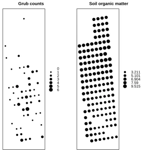
Fig. 1: Left: The observed counts at locations, where the size of the dots corresponds to the grub count (values between 0 and 6). Right: Soil organic matter at location s, where the size of the dots corresponds to the grub count (values from 3.2108 to 9.5146)
IAENG International Journal of Applied Mathematics, 44:3, IJAM_44_3_02
The grub data consists of a set of 142 observations of grub counts with the following variables: longitude, latitude, grub counts and soil organic matter. Figure 1 displays the grub counts (left) and soil organic matter (right) with respect to the given location. An overall negative correlation between the two measures is noticeable, however, the standard regression analysis might be inappropriate as addressed in previous literature. ● ● ● ● ● ● ● ● ● ● ● ● ● ● ● ● ● ● ● ● ● ● ● ●● ● ● ● ● ● ● ● ● ● ● ● ● ● ● ● ● ● ● ●● ● ● ● ● ● ● ● ● ● ● ● ● ● ● ● ● ● ● ● ● ● ● ● ● ● ● ● ● ● ●● ● ● ●●●●● ● ● ● ● ● ● ● ● ● ● ● ● ● ● ● ● ● ● ●● ● ● ● ● ●● ● ●●●●● ● ●● ● ● ●● ● ●● ● ● ●● ● ● ●● ● ●●●● ● ● ● ●
3 4 5 6 7 8 9
[image:5.595.46.283.186.402.2]0 1 2 3 4 5 6 Organic Grub counts
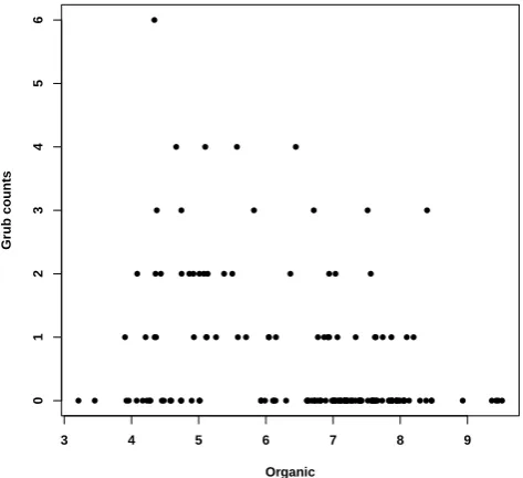
Fig. 2: Scatter Plot of Grub Counts and Organic Matter.
The grub counts take integer values ranging from 0 to 6 and these counts are over-dispersed with an inflated number of zeros. Madsen [21] suggested a negative binomial model for over-dispersed counts and used it to model the ecolog-ical count data under the different biologecolog-ical assumptions (Solomon [25]). Furthermore, Madsen [21] also suggested to use a generalized linear model to estimate regression parameters.
B. Priors for Gaussian Copula Model
For the Japanese Beetle grub data, we use the soil or-ganic matter as the explanatory variable. The explanatory variable X(s) are obtained from the location s given in figure 1. Dalthorp [6] found that a cubic function of the soil organic matter fitted the observed mean grub counts consistently; we will follow the cubic function to model the mean of grub counts. We further include an intercept β0 in the regression parameters β = (β0, β1, β2, β3)T so that
(1, x(s), x2(s), x3(s))T is the co-variate vector associated to variableX(s).
The grub data are modeled by using the Gaussian cop-ula, as defined in Equation(6), to derive the spatially joint distributions with the negative binomial marginal distribu-tions specified in Equation (2). We run Metropolis-Hastings algorithm on the grub data-set with the independent non-informative priors. The priors are
• πβ∼N4((0,0,0,0)T,Σ4×4) • πθ0 ∼Uniform(0,1)
• πθ1 ∼Gamma(0.0001,1000) • πφ∼Gamma(0.0001,1000) • πUi ∼Uniform(0,1)
where the diagonal entries are 104 and the off-diagonal entries are zero for matrix Σ4×4, and i = 1, . . . , n. For posterior simulations, the algorithm is run 12,000 iterations with 6,000 burn-in. On a 3.4 GHz desktop computer, the time with 12,000 iterations is about 6.5 hours. The Gelman-Rubin Statistics in Equation (11) of all the parameters are less than 1.05, indicating that we have a well-defined model and the iterations are sufficiently large.
C. Estimation Performance
Figure 3 shows that the data with the fitted mean function from the Bayesian estimation as well as from the MML esti-mation. The two curves have very similar shapes. The aver-age squared difference in the fitted values is 1421 P142
i=1(ˆyB−
ˆ
yM M L)2 = 0.00053, where yˆB represents the fitted mean from the Bayesian approach andyˆM M L represents the fitted mean from the MML approach.
● ● ● ● ● ● ● ● ● ● ● ● ● ● ● ● ● ● ● ● ● ● ● ●● ● ● ● ● ● ● ● ● ● ● ● ● ● ● ● ● ● ● ●● ● ● ● ● ● ● ● ● ● ● ● ● ● ● ● ● ● ● ● ● ● ● ● ● ● ● ● ● ● ●● ● ● ●●●● ● ● ● ● ● ● ● ● ● ● ● ● ● ● ● ● ● ● ● ●● ● ● ● ● ●● ● ●●●●● ● ●● ● ● ●● ● ●● ● ● ●● ● ● ●● ● ●●●● ● ● ● ●
3 4 5 6 7 8 9
[image:5.595.302.540.336.555.2]0 1 2 3 4 5 6 Organic Grub counts ● Counts MCMC MML
Fig. 3: Plot of observed grub counts as a function of percent soil organic matter. Superimposed is the fitted mean function from both estimation procedures.
The point estimates of the regression coefficients,β, from both the Bayesian approach and the MML method in Madsen [21] are given in Table I. Meanwhile, the numbers in paren-thesis are 95% highest posterior density (HPD) interval (see, i.g., Banerjee et al. [2]) for our Bayesian approach, and a 95% confidence interval for the MML approach, accordingly. The Bayesian analysis concludes that a quadratic function of organic matter is necessary, which is consistent with the result achieved by using the MML method. According to this result, the expected number of grubs given a partic-ular percent organic matter x0 may be best predicted as
exp(−22.37 + 10.88×x0−1.65×x20+ 0.08×x30). Hence, if there is no soil organic matter, then the Japanese Beetle grub count may be best predicted as exp(β0), which is
IAENG International Journal of Applied Mathematics, 44:3, IJAM_44_3_02
close to zero. This result is coincident with the actual facts. The point estimate of the parameter φ is 1.2, which gives
var(Y(s)) = 1.83µ(s). The fitted correlation parameters
[image:6.595.52.284.167.234.2](θ0, θ1) gives a residual correlogram, which is comparable to that in Dalthorp [6].
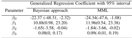
TABLE I: Estimation of the regression coefficients for grub dataset from the Bayesian approach and the MML method, where the MML results are come from Madsen [21] directly.
Generalized Regression Coefficient with 95% interval
Parameter Bayesian approach MML
β0 -22.37 (-48.31, -2.32) -24.34(-47.6, -1.08)
β1 10.88(0.98, 23.20) 11.96(0.54, 23.38)
β2 -1.65(-3.58, -0.04) -1.84(-3.66, -0.02)
β3 0.08(0, 0.17) 0.09(-0.01, 0.19)
By comparing the estimation results of Bayesian approach and MML method, we conclude that:
• Point estimates from the Bayesian approach have small-er absolute values than the estimates from the MML approach. In addition, all intervals from the Bayesian approach are consistently narrower than corresponding intervals from the MML method.;
• Unlike the MML intervals, all the intervals from our Bayesian approach are “significant” in the sense that they do not span over zero;
• In Bayesian approach, Bayesian updating is widely used and computationally convenient; while in MML method, the computational complexity from using the maximum likelihood (ML) algorithm to obtain the ML estimates of the variance components and their derivatives signif-icantly increase the computational burden.
D. Prediction Performance
To assess the accuracy of Bayesian prediction, we also implemented the GAM prediction as a comparison. Gen-erally, GAM gives us a non-integer fitted mean as the prediction, and we call this non-integer prediction as the GAM mean prediction; while Bayesian prediction yields the integer prediction. In order to make a sensible comparison among them, we introduce two common methods to get the GAM integer prediction:
[image:6.595.312.541.239.311.2]Method 1: Rounding the fitted mean to the closest integer; Method 2: Using the fitted median as the prediction. For simplicity, we will call method 1 and method 2 as “GAM rounding prediction” and “GAM median prediction”, respectively.
TABLE II:MSPEvalues from both Bayesian prediction and two common GAM integer predictions with 10%, 20% and 44% of missing data.
MSPEs
Bayesian Two common GAM integer predictions Missing prediction rounding median
10% 1.71 1.71 1.79
20% 1.18 1.21 1.32
44% 1.68 1.48 1.74
In the application to the grub data set, we randomly hold out 10%, 20% and 44% of the data and use the remainder to
make prediction. And we use theMSPEdefined in Equation (15) as the performance criterion. Table II gives us theMSPE
values between the predicted values and the true values for both Bayesian prediction and two common GAM integer predictions (i.e., GAM rounding prediction and GAM median prediction). Bayesian prediction (2ndcolumn) is close to the GAM rounding prediction (3rd column). However, Bayesian prediction gives a more accurate prediction than the GAM median prediction (4thcolumn), since all theMSPE values from Bayesian prediction are less than the corresponding values from GAM median prediction.
TABLE III: Decomposition of comparison between Bayesian prediction and GAM mean prediction to zero and non-zero group
Category 1:Y = 0 Category 2:Y >0
Bayesian GAM mean Bayesian GAM mean
Missing prediction prediction prediction prediction
10% 0.20 0.52 5.50 4.74
20% 0.20 0.38 2.31 1.82
44% 0.14 0.30 3.67 2.81
It is notable that about 50% of the counts are 0 in grub data. Therefore, it seems sensible to divide the missing count data into two groups, zeros and non-zeros. The performance of Bayesian prediction is explored separately in each of these two groups. For the sake of simplicity, here we only discuss the comparison between Bayesian prediction and traditional non-integer GAM prediction, i.e., GAM mean prediction. Table III givesMSPEs for both zeros and non-zeros group. Obviously, for the zero-count data, Bayesian prediction is significantly better than the GAM mean prediction.
V. SIMULATION
We further evaluate the performance of Bayesian predic-tion against the GAM predicpredic-tion with the simulated data. We generate the data on a regular square grid with unit spacing. Two sample sizes are simulated (n = 144 and
n = 225). For each sample size, two levels of spatial dependence (moderate and strong) are simulated, where the spatial dependence is specified by the effective range (see, Madsen [21]). The moderate and strong dependence have the effective ranges R = 8.3 and R = 14, respectively. In this simulation study, all the target means are set to be a constant, i.e., exp(1). Hence, the dependence in the data is not from the spatial pattern of the co-variate, but from spatial proximity ( Madsen [21]). As before, we randomly hold out 10%, 20% and 44% of the observations, and use the re-mainders to predict them. Therefore, there are altogether2× 2×3(the number of observation×the number ofRlevel×
the number of holdout percent) scenarios. For each scenario, 50 data sets are generated for each scheme, then the mean of MSPE is used as the criterion of measure prediction performance. Furthermore, in each scenario, the locations of the missing data are set to be the same for all 50 simulated data sets.
Accordingly, the priors are specified as πβ ∼N(0,104),
πθ0 ∼Uniform(0,1), πθ1 ∼Gamma(0.0001,1000), πφ ∼
Gamma(0.0001,1000), πU ∼ Uniform(0,1). And 20,000 iterations with 10,000 burn-in are run for each scenario.
IAENG International Journal of Applied Mathematics, 44:3, IJAM_44_3_02
[image:6.595.57.281.680.750.2]TABLE IV:Comparison of Bayesian prediction and two common GAM integer predictions, predicting 10%, 20% and 44% missing from simulated data
mean ofMSPEs (sd) Sample Effective Percent Bayesian GAM integer predictions
Size Range Missing prediction rounding median
10% 1.28 (0.48) 1.45 (0.67) 1.52 (0.65) R=14 20% 1.27 (0.38) 1.42 (0.45) 1.45 (0.44) 44% 1.44 (0.38) 1.57 (0.44) 1.62 (0.42)
N=225
10% 2.12 (0.92) 2.25 (0.96) 2.26 (1.02) R=8.3 20% 2.14 (0.60) 2.20 (0.58) 2.25 (0.67) 44% 2.24 (0.49) 2.33 (0.541) 2.33 (0.537)
10% 1.44 (0.74) 1.72 (1.08) 1.73 (1.18) R=14 20% 1.35 (0.54) 1.56 (0.63) 1.63 (0.66) 44% 1.58 (0.61) 1.74 (0.65) 1.78 (0.72) N=144
10% 2.17 (0.92) 2.22 (0.98) 2.31 (1.04) R=8.3 20% 2.29 (0.95) 2.33 (0.96) 2.42 (1.00) 44% 2.30 (0.60) 2.43 (0.72) 2.51 (0.75)
Table IV lists the mean of 50 MSPEs with the standard deviation for both Bayesian prediction and two common GAM integer predictions. All the values obtained from Bayesian prediction (4th column) are significantly smaller than the values obtained from two common GAM integer predictions, i.e., GAM rounding prediction (6th column) and GAM median prediction (7thcolumn). Hence, Bayesian prediction is thus much better than two common GAM integer predictions. Moreover, most standard deviations for
MSPEs from Bayesian prediction are less than the values from two common GAM integer predictions, which indicates Bayesian prediction is more efficient than two common GAM integer predictions. Moreover, the MSPEs from Bayesian prediction decrease as the effective range increases (from
R = 8.3 toR = 14) or as the sample size increases (from
n= 144 ton= 225).
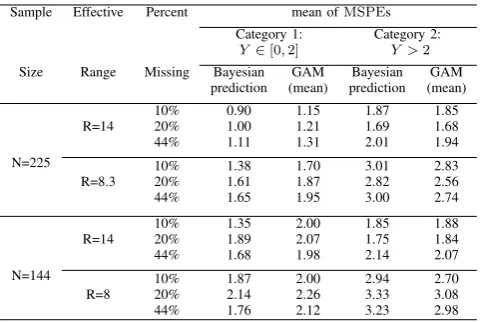
[image:7.595.50.292.589.750.2]Like the method used in the real-life data analysis, we divide the simulated count data into two categories, one with counts less than or equal to 2 and the other with counts over 2. The reason for using 2 as the cut-off point is that the simulated count data are typically larger than 0. For simplicity, we do the comparison between the Bayesian prediction and the GAM mean predictions only.
TABLE V:Decomposition of comparison between Bayesian pre-diction and GAM mean prepre-diction to two groups: no more than 2 and more than 2
Sample Effective Percent mean ofMSPEs Category 1: Category 2:
Y ∈[0,2] Y >2
Size Range Missing Bayesian GAM Bayesian GAM prediction (mean) prediction (mean)
10% 0.90 1.15 1.87 1.85 R=14 20% 1.00 1.21 1.69 1.68 44% 1.11 1.31 2.01 1.94
N=225 10% 1.38 1.70 3.01 2.83 R=8.3 20% 1.61 1.87 2.82 2.56 44% 1.65 1.95 3.00 2.74
10% 1.35 2.00 1.85 1.88 R=14 20% 1.89 2.07 1.75 1.84 44% 1.68 1.98 2.14 2.07 N=144 10% 1.87 2.00 2.94 2.70 R=8 20% 2.14 2.26 3.33 3.08 44% 1.76 2.12 3.23 2.98
Table V lists the mean of 50 MSPEs for both Bayesian prediction and GAM mean prediction by firstly splitting
the missing count into two groups. As seen from Table V, Bayesian prediction and the GAM mean prediction come to a tie for large count category, i.e.,Y >2. However, Bayesian prediction performs consistently better than the GAM mean prediction for the smaller count category, i.e.,Y ≤2. Hence, Bayesian approach may give better prediction in application to predict the small-count data.
VI. DISCUSSION ANDCONCLUSION
We develop a Bayesian approach which performs parame-ter estimation and spatial prediction simultaneously. Building on top of a copula model, an MCMC scheme (Metropolis-Hastings Algorithm plus rejection sampling) is adopted to iteratively update parameter estimates. Upon convergence the parameters are then used for spatial (missing count data) prediction.
As for parameter estimation, we compare to the MML method in Madsen [21] in the same real-life data-set (Grub Data). Our Bayesian approach yields narrower confidence intervals, which always do not span over zero. This implies that our results are more precise and robust.
Moreover, we compare the spatial (missing count) predic-tion to the common Generalized Additive Models (GAM). We carry out experiments on the real-life data-set, as well as a simulated data-set with many different settings. For practical considerations, we categorize the missing counts into small value and large-value groups. The experiment results demonstrate that our approach outperforms GAMs in almost all settings, especially when the missing data is small. Although we demonstrate the usage of our Bayesian ap-proach in spatially correlated discrete data, the methodology is general and can be easily applied in other correlated (count) data, including temporally correlated data.
ACKNOWLEDGMENT
The author acknowledge the financial support from Shang-hai University of International Business and Economics. The authors would like to thank an anonymous referee for his or her constructive comments and suggestions.
REFERENCES
[1] H. Assareh and K. Mengersen, “Bayesian estimation of the time of a decrease in risk-adjusted survival time control charts”, IAENG International Journal of Applied Mathematics, 41(4), pp. 360-366, 2011.
[2] S. Banerjee, B.P. Carlin and A.E. Gelfand, “Hierarchical Modeling and Analysis for Spatial Data”,Chapman & Hall/CRC, 2004.
[3] J.M. Bernardo and A.F.M. Smith, “Bayesian Theory”.Chichester: John Wiley & Sons Ltd, 1994.
[4] J.O. Berger, V. De Oliveira, and B. Sans´o, “Objective Bayesian anal-ysis of spatially correlated data”.Journal of the American Statistical Association, 96(456), pp. 1361-1374, 2001.
[5] N. Cressie, “Statistics for Spatial Data”. revised ed.,John Wiley and Sons, Inc., 1993.
[6] D. Dalthorp, “The generalized linear model for spatial data: assessing the effects of environmental covariates on population density in the field”. Entomologia Experimentalis et Applicata, 111, pp. 117-131, 2004.
[7] D. Dalthorp, J. Nyrop and M. Villani, “Spatial ecology of the japanese beetle”. Popillia japonica, Entomologia Experimentalis et Applicata, 96, pp. 129-139, 2000.
[8] M. Denuit and P. Lambert, “Constraints on concordance measures in bivariate discrete data”.Journal of Multivariate Analysis, 93, pp. 40-57, 2005.
[9] P.J. Diggle, P.J. Ribeiro and O.F. Christensen, “An introduction to model-based geostatistics”.Spatial statistics and computational meth-ods. Springer New York, pp. 43-86, 2003.
IAENG International Journal of Applied Mathematics, 44:3, IJAM_44_3_02
[10] M.D. Ecker and A.E. Gelfand, “Bayesian Variogram Modeling for an Isotropic Spatial Process”.Journal of Agricultural, Biological and Environmental Statistics, 2, 347-369, 1997.
[11] J. Eidsvik, A.O. Finley, S. Banerjee, et al, “Approximate Bayesian inference for large spatial datasets using predictive process models”. Computational Statistics & Data Analysis, 56(6), pp. 1362-1380, 2012. [12] Y. Fang and L. Madsen, “Modified Gaussian pseudo-copula: Appli-cations in insurance and finance”.Insurance: Mathematics and Eco-nomics, 53(1), pp. 292-301, 2013.
[13] Y. Fang, L. Madsen and L. Liu, “Comparison of Two Methods to Check Copula Fitting”. IAENG International Journal of Applied Mathematics, 44(1), pp. 53-61, 2014.
[14] A. Gelman, G.O. Roberts and W.R. Gilks, “Efficient Metropolis jumping rules”.Bayesian Statistics, 5, 599-608, 1996.
[15] W.R. Gilks, S. Richardson and D.J. Spiegelhalter, “Inference and monitoring convergence”. Markov Chain Monte Carlo in Practice, Chapman and Hall/CRC, Boca Raton, Florida, 131-143, 1996. [16] S. Gschl¨oßl and C. Czado, “Does a Gibbs sampler approach to spatial
Poisson regression models outperform a single site MH sampler?” Computational Statistics and Data Analyis, 52, 4184-4202, 2008. [17] T.J. Hastie and R.J. Tibshirani,Generalized Additive Models, Dept. of
Statistics Technical Report No. 2, Stanford University, 1984. [18] P. Hougaard, M.L. Lee, and G.A. Whitmore. “Analysis of
overdis-persed count data by mixtures of Poisson variables and Poisson pro-cesses”. Biometrics, 53(4), pp. 1225-1238, 1997.
[19] J.P. LeSage, M.M. Fischer, and T. Scherngell, “Knowledge spillovers across Europe: evidence from a Poisson spatial interaction model with spatial effects”.Papers in Regional Science, 86, 393-422, 2007. [20] K.Y. Liang and S. Zeger, “Longitudinal data analysis using generalized
linear models”.Biometrika, 72, pp. 13-22, 1986.
[21] L. Madsen, “Maximum Likelihood Estimation of Regression Parame-ters With Spatially Dependent Discrete Data”.Journal of Agricultural, Biological, and Environmental Statistics, 14, pp. 375-391, 2009. [22] J.F. Monahan,Numerical methods of statistics, Illustrated, Cambridge
Univ Pr, 371, 2001.
[23] M. Pitt, D. Chan and R. Kohn, “Efficient Bayesian inference for Gaussian copula regression models”.Biometrika, 93, pp. 537-554, 2006. [24] A. Sancetta, “Universality of Bayesian Predictions”.Bayesian
Analy-sis, Volume 7, pp. 1-36, 2012.
[25] D.L. Solomon, “The Spatial Distribution of Butterfly Eggs”. Life Science Models, Vol. 4, eds. H. Roberts and M. Thompson, New York: Springer-Verlag, pp. 350-366, 1983.
[26] P.X.K. Song, M.Y. Li and Y. Yuan, “Joint regression analysis of correlated data using Gaussian copulas”.Biometrics, 65(1), pp. 60-68, 2009.
[27] H. Strasser, “Consistency of Maximum Likelihood and Bayes Esti-mates”.Annals of Statistics, 9: 1107-1113, 1981.
[28] S. Zeger and K.Y. Liang, “Longitudinal Data Analysis for Discrete and Continuous Outcomes”.Biometrics, 42, 121-130, 1986.