On the validation of solid mechanics models using optical measurements and data decomposition

On the validation of solid mechanics models using optical

measurements and data decomposition

LAMPEAS, George, PASIALIS, Vasileios

<http://orcid.org/0000-0002-2346-3505>, LIN, Xiaoshan and PATTERSON, Eann

Available from Sheffield Hallam University Research Archive (SHURA) at:

http://shura.shu.ac.uk/11867/

This document is the author deposited version. You are advised to consult the

publisher's version if you wish to cite from it.

Published version

LAMPEAS, George, PASIALIS, Vasileios, LIN, Xiaoshan and PATTERSON, Eann

(2015). On the validation of solid mechanics models using optical measurements

and data decomposition. Simulation Modelling Practice and Theory, 52, 92-107.

Copyright and re-use policy

See

http://shura.shu.ac.uk/information.html

Sheffield Hallam University Research Archive

On the validation of solid mechanics models using optical measurements and

data decomposition

G. Lampeas

, V. Pasialis

, X. Lin

and E. A. Patterson

1. Laboratory of Technology and Strength of Materials, Mechanical Engineering and Aeronautics Department, University of Patras, 26500 Rion, Greece, email: [email protected]

2. School of Engineering, University of Liverpool, Brownlow Hill, Liverpool, L69 3GH, UK email: [email protected]

Abstract

Engineering simulation has a significant role in the process of design and analysis of most engineered products at all scales and is used to provide elegant, light-weight, optimized designs. A major step in achieving high confidence in computational models with good predictive capabilities is model validation. It is normal practice to validate simulation models by comparing their numerical results to experimental data. However, current validation practices tend to focus on identifying hot-spots in the data and checking that the experimental and modeling results have a satisfactory agreement in these critical zones. Often the comparison is restricted to a single or a few points where the maximum stress / strain is predicted by the model. The objective of the present paper is to demonstrate a step-by–step approach for performing model validation by combining full-field optical measurement methodologies with computational simulation techniques. Two important issues of the validation procedure are discussed, i.e. effective techniques to perform data compression using the principles of orthogonal decomposition, as well as methodologies to quantify the quality of simulations and make decisions about model validity. An I-beam with open holes under three-point bending loading is selected as an exemplar of the methodology. Orthogonal decomposition by Zernike shape descriptors is performed to compress large amounts of numerical and experimental data in selected regions of interest (ROI) by reducing its dimensionality while preserving information; and different comparison techniques including traditional error norms, a linear comparison methodology and a concordance coefficient correlation are used in order to make decisions about the validity of the simulation.

Keywords

Digital Image Correlation, Full-field measurements, Zernike moment descriptor, Simulation, Validation, Concordance coefficient.

1.

Introduction

Engineering simulation is used extensively in the process of design and analysis of engineered products at all scales to provide elegant designs optimized for cost, life and weight. Despite the development of easy-to-use finite element programs, it is still a complex task to create computational models that enable accurate representations of the physical reality; therefore the reliable prediction of design quantities (i.e.

2

represent a complex physical reality at an affordable computing time and cost involves many assumptions about model parameters, which introduce uncertainty to the modeling process. To overcome the lack of credibility in simulations in cases where a high level of confidence in the design is required, the simple solution of conservative design is followed. However, this practice requires increased material usage, resulting in increased product cost and structures with large ecological footprints.

Major steps in achieving high confidence in the predictive capabilities of computational models are the model verification and validation. Verification is defined as ‘the process of determining that a computational model accurately represents the underlying mathematical model and its solution' [1]. Software code

developers mostly deal with the issue of verification, through the extensive comparison between numerical and analytical solutions, so as to prove that the model equations have been properly introduced and solved within the code. Whereas, validation is defined as 'the process of determining the degree to which a model is an accurate representation of the real world from the perspective of the intended uses of the model' [1]; this implies that the model should represent the real structural behavior with sufficient accuracy, therefore, it always needs reference to experimental tests.

Current validation practices tend to focus on identifying hot-spots in the data and checking that the experimental and modeling results have a satisfactory agreement in these critical zones. Often the comparison is restricted to a single or a few points where the maximum stress / strain is predicted by the model. This highly localized approach is the result of traditional strain measurement methodologies using strain gauges, but neglects the majority of the data generated by numerical analysis, carrying with it the risk that critical regions may be missed all together. For example, Jin et al [2] used digital image correlation (DIC) to acquire a full-field map of strain in rectangular blocks of polyurethane foams subject to compression between steel plates; however, the quantitative comparison of simulation and experimental displacement fields was limited to selected sections in the specimen. Similarly, Spranghers et al [3] made full-field measurements and used inverse methods to identify the plastic behavior of aluminum plates subject to free air explosions; but

quantitative comparison between simulation data and experimental results was also limited to selected point locations, despite the availability of full field data.

Optical measurement technologies have reached a readiness level, due to recent developments, that enable displacement or strain data over large areas, or even the entire structure, to be reliably captured during an experimental test and thereafter visualized and analyzed. For example, Digital Image Correlation (DIC), Digital Speckle Pattern Interferometry (DSPI) and shearography are steadily replacing conventional measurement techniques such as strain gauges and extensometers [4]. Such developments provide the background for a more comprehensive approach to model validation, which could lead to optimized and less conservative designs. Although many companies have developed internal procedures for comparing simulation results to experimental data, there are no standard procedures for the validation of computational solid mechanics models used in engineering design. In the EU research project ADVISE [5], a methodology for validation of computational solid mechanics models based on full field data comparisons was developed [6]. In a subsequent European Union supporting action project VANESSA [7], the appropriateness of this validation procedure as part of a regulatory process for validation of computational solid mechanics models was examined.

difficulties, sensitivities and implementation issues related to the validation methodology have been revealed and further improvements of the methodology towards its whole field application are proposed.

2.

Three point bending of perforated I-beam: testing and modeling

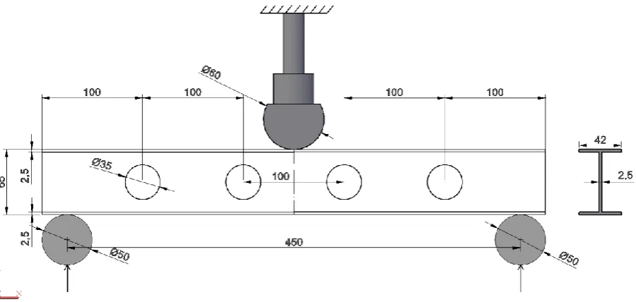
The three-point bending of an aluminum I-beam is shown schematically in Figure 1. Despite its simple geometry, the perforated I-beam has many interesting structural analysis features, such as high stress concentrations around the holes, local plasticity in the contact areas and geometric - material non-linearity due to contact at the indenter and supports. The material properties of the aluminium beam are presented in

Table 1. For the experimental purposes, an MTS testing machine capable of delivering up to 250kN normal force was used and the beam was placed on two rigid cylindrical supports that were 450mm apart. A steel rod was used to apply a nominally static vertical force at the mid-point of the beam. Additionally, a stereoscopic DIC system (Aramis 5M [8]) was employed to measure displacements during the loading event, using images acquired at a frequency of 15 frames per second. Strain fields were calculated from the displacement

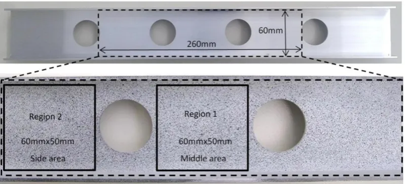
measurements for a region of interest (ROI) on the beam web (260mmx60mm), covering the contact location and the area around the holes, as shown in Figure 2, with the aim of including all of the regions of stress concentration and the contact zones. Prior to testing, a random black and white speckle pattern was sprayed onto the region of interest. The structural and optical experimental setup is shown in Figure 3.

Figure 1: Drawing of the aluminum I-beam specimen, loading and support rods (dimensions in mm)

Table 1: Al6060 material properties Material

Designation

Ultimate strength Rm (MPa)

Yield stress Rp0. 2 (MPa)

Elongation to failure A%

Young modulus E (GPa)

4

Figure 2: Selected region and sub-regions of interest (ROI) for optical measurements.

Figure 3: Experimental setup for testing of I-beam

During the post-processing of the images, the facet size and pitch were set to 46 and 11 pixels,

respectively, while the strain parameter was set to 11, meaning that strain was calculated for an area of 11x11 facets or displacement vectors. The larger the size of the facet, the better the accuracy of the displacement result, so facets were overlapped to provide good quality and high density displacement data at the cost of increased computational time [8]. The strain parameter acts as an effective strain gauge-length and also as a noise reduction parameter, because it controls the area of the strain calculation, but at the same time an increase in the parameter can decrease the accuracy of results. The strain accuracy of the ARAMIS 5M system is generally considered to lie within the conservative limits of ±0.05% [8]. However, as the minimum

measurement uncertainty value is a critical parameter in the model validation process, the DIC system was calibrated before taking optical measurements, using an appropriate reference material, according to the procedures described in [9] and [10]; this calibration has resulted in a more precise determination of the measurement uncertainty, which was 10μm for displacement and 30με for strain measurements, respectively.

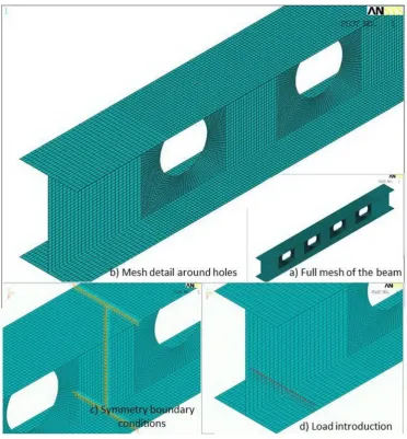
mesh was generated around the open holes (Figure 4b), as in these areas high strain gradients were expected. Boundary conditions were introduced at the supports in terms of displacement constraints in the y-direction. Furthermore, symmetry conditions around the y-axis were assumed in order to provide numerical stability during the solution process (Figure 4c). The total applied force of 9.8kN was distributed along two lines on the bottom flange, (Figure 4d). The beam material was represented by an elasto-plastic material model with kinematic hardening. Post-processing of the model results included calculating full-field displacement and strain contour plots for the beam, which were used for comparison with the corresponding experimental results at the selected region of interest.

Figure 4: Details of the mesh used for the computational model of the I-beam

3.

Decomposition of displacement and strain fields

6

However, even when a point-to-point comparison is achieved, it may lead to a result that is difficult to interpret from the point of view of model validation.

Since there is often a high level of redundancy in the raw data from both experiments and simulations, there is an opportunity to perform data compaction to retain only the 'useful' information before attempting a comparison process. An efficient means for performing this task is to handle strain and displacement data fields as images and apply image decomposition techniques based on orthogonal polynomials. Ideas

originating from image analysis and processing e.g. for fingerprint recognition [11] and human face recognition [12] can be appropriately adapted for this purpose. Orthogonal decomposition to reduce the dimensionality of ‘raw’ data has been recently applied to displacement and strain image decomposition [13-15], as well as to finite element model updating [16]. Orthogonal polynomials, such as Zernike, Tchebichef or Krawtchouk are advantageous because they are very effective in data reduction and are also invariant to scale, rotation and translation, thus enabling direct comparison of results regardless of whether the data fields are in the same coordinate system, have the same scale, orientation, or sampling grid. The decomposed feature vector should ideally comprise between twenty and hundred terms and be information-preserving, such that most of the useful information is retained, in order to permit a meaningful comparison of experimental results with those from simulation and to obtain an insight into the structural response.

The Zernike polynomial decomposition, which is applied in the current validation exemplar, is presented in more detail hereafter. Let represent a matrix containing the values of the quantity of interest at location

( , )

 

(1)

However, as reconstruction of an image using an infinite number of Zernike moments is not practical, an approximate reconstruction may be achieved by retaining a finite number of moments from the order 0 to order Nmax and discarding the remaining higher order Zernike polynomial terms:

(2)

In equations (1) and (2), are Zernike moment descriptors, given by

(3)

and

(4)

where, m and n are integers subject to constraints even and , while,

( , ) 

I

( , )

 

I I( , ) 

, , 0

( , ) n m n m( , ) n m

I

 

 

  



( , ) _{n m n m}( , ) n m

I

 

 

  



Z

( , )

( )

n m n m

V

 



R



e

nm m n 2 1 * , , 0 0 1 ( , ) ( , )

n m n m

n

Z I V d d



 

    





(5)

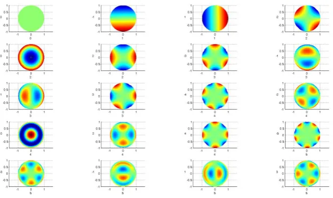
and n is a non-negative integer representing the order of the radial polynomial R(ρ). The first 20 terms of Zernike polynomials are shown schematically in Figure 5.

Figure 5: Schematic of the 20 first terms of the Zernike polynomials

Moreover, the rotational invariance of the Zernike polynomials can be further exploited by calculating only the positive terms (m≥0), [17]:

(6)

The quality of the reconstruction depends on the number, Nmax of Zernike moments used for the image

description. The appropriate selection of the Nmax value can be determined by using a predefined tolerance

when comparing the original image with its reconstruction. An increase in the value of this tolerance results in a higher image compaction by retaining fewer shape descriptors, but the potential loss of image information is higher. In order to assess the accuracy of the Zernike decomposition, the Pearson coefficient or correlation error [18] may be used

(7) where and are given as:

( )/2

2 ,

0

(

)!

( )

( 1)

!

!

!

2

2

n m

s n s

n m

s

n s

R

n

m

n

m

s

s

s











 

  









 





 







 



, 0

0

2 ( ) Re cos( ) Im sin( ) Re Im ( )

N M

n m n m n n

n m n

n m

I R  Z m Z m Z j Z R 



       





( , )

corr I I

 

 

 





2

ˆ ˆ ˆ

ˆ ˆ ( , )

I I I I dA

corr I I

I I dA I I dA

8

Alternatively, the normalized mean root square error,

e

(8)

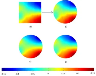
In the present study, 400 Zernike moments were used initially in the decomposition process, as when the maximum number of Zernike moments exceeds 450 to 500 terms, numerical instabilities may occur and special techniques e.g. [20, 21] are required. Further data compression was performed by retaining only the most important Zernike moments. It was assumed that a measure of a moment’s contribution to the image description was its magnitude and therefore to achieve further data compression only the highest terms were retained. In all cases, the number of Zernike moments needed for efficient image description depends on the image content and not on the number of data points which is controlled by the data acquisition processes. Αn example of the decomposition process for a ‘DIC image’, i.e. a strain data-field obtained using digital image correlation, is shown schematically in Figure 6. An interesting observation about the DIC image in Figure 6 is that despite the adjustment of the strain parameter in the DIC data post-processing, a significant amount of noise is still present Figure 6(a). Further noise reduction can be achieved by retaining less Zernike moment terms with the drawback of a higher reconstruction error Figure 6(b, c, d).

Figure 6: Schematic presentation of the decomposition process. a) Original DIC image or strain data-field b) Reconstructed unit disc image with 400 Zernike terms (e=0. 35%) c) Reconstruction with 16 terms (e=4%) d)

Reconstruction with 50 terms (e=1. 65%).

The moments can be collated together as terms in a vector, which is sometimes known as a feature vector. Then, the image data have been reduced in dimension from a two-dimensional matrix containing thousands of

, ˆ

ˆ  

 

 IdA  IdA

I I

dA dA

∬

∬

∬

∬

[

]

2

( , ) ( , )

( , ) D

D

I x y I x y dxdy

e

I x y dxdy

∬

∬

-=

elements to a one-dimensional vector containing tens of terms. It is important for the comparison process that the data fields from the finite element study and digital image correlation are decomposed using the same process resulting in a feature vector with the same number of terms; and a perfect alignment of regions of interest (ROI) between the experimental and the simulation images is an essential requirement.

The feature vector representing the data from experiment is created from the subset of m largest Zernike moments obtained from the decomposition, where m is the smallest number of moments that will give a correlation coefficient between the reconstructed and original image that is within the specified tolerance; and the corresponding feature vector representing the results from the simulation is created in the same way but from the n largest Zernike moments such that m and n are not necessarily equal and the rank order of the two sets of Zernike moments are not necessarily the same. Hence, before the two feature vectors from the experiment and the simulation are ready for comparison, some extra moments need to be appropriately selected, such that both vectors contain equal numbers of terms with one-to-one correspondence.

4. Methods for comparison experimental and simulation data

4.1 Qualitative data comparison

Typical plots of full-field displacement data calculated by the FE model and measured using DIC are shown in Figure 7 and it may be observed, that the open-holes in theDIC images appear to have a slightly larger diameter, because the digital image correlation process could not be extended to the hole edges due to the finite size of the facets. Therefore, a narrow annular region around the holes has to be excluded from the strain computation [8].

Figure 7: Maps of displacement (mm) in the x-direction from a) FE model b) DIC measurements

The presence of open holes in the web causes difficulties in decomposing the images using moment descriptors. Decomposition using orthogonal polynomials is possible for arbitrary geometry, even in cases of non-planar shapes including holes or cutouts, e.g. by using Adaptive Geometric Moment Descriptors (AGMD); however this is a highly case dependent process, which requires a specific treatment of each individual

10

to continuous circular or rectangular planar regions; for this reason data comparison was initially performed for two rectangular areas of the I-beam, namely “Region 1” and “Region 2”shown in Figure 2. Subsequently to achieve whole field validation, two techniques based on Zernike decomposition were considered in section 5, namely ‘patchwork’ and ‘hole-interpolation’.

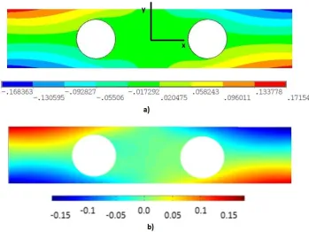
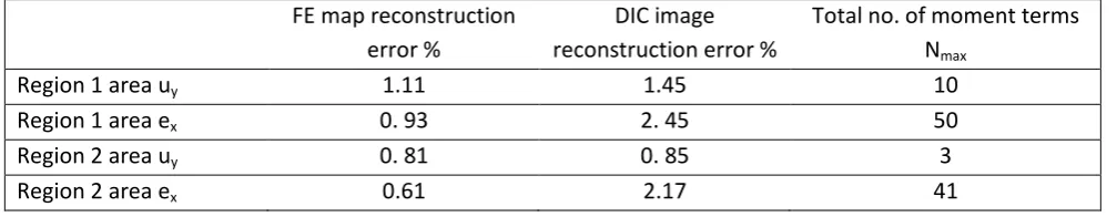
In Figure 8, both numerical and experimental data for displacements in the y-direction and normal strain in the x-direction, are shown for “Region 1” and “Region 2”. In Table 2, the total number of Zernike terms, Nmax, as well as the reconstruction errors for the decomposition process are presented and indicate that in all

the studied cases the reconstruction error is lower than the predefined tolerance of 3%. It can be also observed that the number of moment terms retained is small, ranging from 50 down to only 3 terms, thus enabling a more straightforward comparison and validation process.

Figure 8: Maps of y-direction displacement, uy (mm) and x-direction strain, x (%) from the finite element

model (top) and digital image correlation (bottom) for Regions 1 and 2, shown in Figure 2.

Figure 8 can be used for a qualitative comparison between the experimentally-derived and numerically-calculated data fields and it may be concluded that there is good agreement between the results from experiment and simulation. However, model validation requires quantitative assessment of the validity of computational models; three different methodologies to realize such quantitative comparisons are discussed in sections 4.2, 4.3 and 4.4.

Table 2: FE and DIC data: normalized reconstruction errors and number of retained terms FE map reconstruction

error %

DIC image reconstruction error %

Total no. of moment terms Nmax

Region 1 area uy 1.11 1.45 10

Region 1 area ex 0. 93 2. 45 50

Region 2 area uy 0. 81 0. 85 3

4.2 Error norm comparison

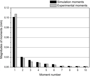
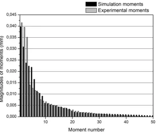
In Figure 9 the feature vector terms representing the displacement and strain fields, respectively, from the simulation and experiment are presented. A traditional way of comparing experimental and simulation results is to calculate differences using error norms. Adapting this approach to the present case and taking into account that the DIC and FE displacement and strain maps have been decomposed, the error norm of the feature vector terms has been calculated. The error norm calculation is much simpler after decomposition, because instead of millions there are only tens of values to be processed.

12

Figure 9b: Magnitude of the moments or terms in the feature vector representing the x-direction strain, x in Figure 8 for Region 1 in Figure 2.

The error norm is calculated as the average difference between the moments representing the results from the simulation, mSi and experiment, mEi, which is mathematically expressed as

(9)

In expression (9) all of the moments are considered to be equally important, resulting in a potentially distorted comparison. A more meaningful approach is to calculate the weighted average of differences, taking into account the contribution of each moment to the image reconstruction. Since the measure of a moment’s contribution is its magnitude, a normalization weighting parameter pi can be introduced, which takes into

consideration the importance of each moment, while the sum of all pi parameters must be equal to unity.

Therefore, each deviation di is multiplied by a respective weighting parameter pi resulting in the following

expression

(10)

For each moment, the weighting parameter is expressed by the ratio of the magnitude of the moment to the sum of all moments:

1

Average deviation 1 1 100%

N

i i mean i

i i

d d mS mE

N N  mE



 



1

Weighted average deviation

N wmean i i

i

d

d p



(11)

and

(12)

While this can be done independently for moments from the simulation and experiment, it is more appropriate to use an average value for the moment pair such that the sum of average values of the normalization parameters remains equal to unity, i.e.

(13)

Hence combining Equations (10) and (12) leads to the following expression for the weighted average deviation

(14)

The weighted and non-weighted average deviations for the displacements and strain fields in regions 1 and 2 are presented in Table 3, from which general indications about the model quality may be drawn, although the type of error norm applied (weighted or non-weighted) influences significantly the conclusion.

uexp

Region 1 u_y 11. 52% 8. 9% 2.69%

x 28. 36% 22. 93% 3.57%

Region 2 u_y 1. 05% 4. 98% 2.73%

x 27. 72% 12. 79% 3.97%

Table 3: Weighted and non-weighted average deviation based on equations (10) and (14) respectively, for the moments representing the displacement and strain data fields for the regions shown in Figure 2.

It should be noted that consideration of the average deviations of the results from simulation and experiment does not allow a definite decision about the validity of the simulation to be made. A further step is required, such as relating these deviations to the errors in the experimental results which can be evaluated from a calibration of the DIC system, the errors resulting from the image decomposition process, as well as any other uncertainties originating from either the simulation or experimental processes. The relative uncertainty, urel in in-plane DIC measurements have been assessed previously [9] to have an average value of 2.6% and this

1

Simulation normalized parameter _{i N} i

i i S

mS

mS





Experimental normalized parameter _{i N} i

i i E

mE

mE





i N N

i i i i mS mE p mS mE               





i i i i

w mean N N

i

i i

i i

d mS mE mS mE

mE mS mE                     







14

can be combined with the error in the decomposition process, udeco given in Table 2, to produce a measure of

the error or uncertainty in the experimental data, uexp where

𝑢_𝑒𝑥𝑝 = √𝑢_𝑟𝑒𝑙2 _{+ 𝑢} 𝑑𝑒𝑐𝑜

2 ₍₁₅₎

It may be remarked from Eq. (15), that when the DIC measurements have a high relative uncertainty urel, an

increase of the total experimental uncertainty occurs, resulting to a false increase of the level of fidelity of the simulation; a similar effect would occur with a large error from the decomposition / reconstruction process, e.g. when fewer number of moment descriptors are included in the reconstruction calculation, or if certain strain patterns are not well-represented by the Zernike moment descriptor. In order to avoid an artificial increase in the simulation accuracy due to an increase in the experimental uncertainty, independent

limitations were imposed on both uncertainty values urel and udeco, to keep them as small as possible, such that

the total experimental uncertainty (Eq. 15) is also kept very small. Specifically, in the present I-beam validation, reconstruction errors were kept to very small values, as shown in Table 2; furthermore, the experimental uncertainty was also low, i.e. 10μm for displacement and 30 με for strain measurements, respectively. The recently published CEN guide on validation [10] recommends that the error arising from the decomposition process should be less than the experimental uncertainty and highlights that minimum

measurement uncertainty in an experiment is likely a function of the cost of the experiment, i.e. the investment in equipment, training and time spent conducting the equipment.

In Table 3, it can be observed that the weighted and unweighted differences for the strain data in both regions are many times greater than the experimental uncertainty and hence it can be concluded that the differences are significant and the quality of the model is not good. The differences for the displacement data are smaller and for Region 2 of the same order as the experimental uncertainty, so it could be concluded that the difference is not significant and the model is a good representation of the experiment. This crude

assessment can be confirmed by qualitative visual inspection of the data fields in Figure 8.

4.3 Linear correlation comparison

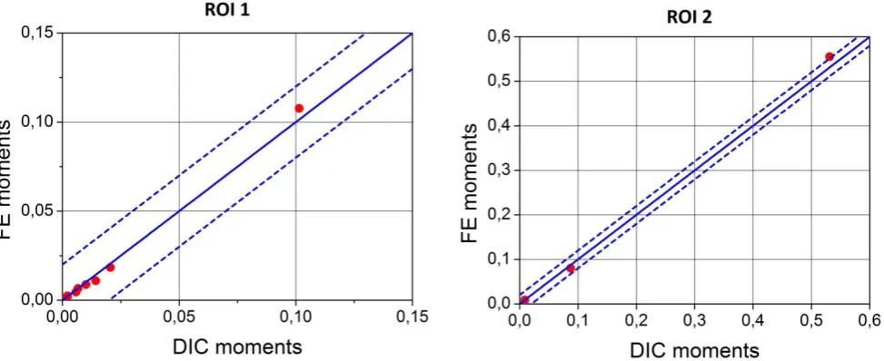
Figure 10a: Zernike moments representing y-direction displacement fields, uy from the FE model plotted as a

function of the Zernike moments representing the corresponding data field from the experiment for Regions 1 and 2 in Figure 2; the solid line is mE=mS and the broken lines show mS=mE2u.

Figure 10b: Zernike moments representing x-direction strain x from the FE model plotted as a function of

Zernike moments representing the corresponding data field from the experiment for Regions1 and 2 in Figure 2; the solid line is mE=mS and the broken lines show mS=mE2u.

It becomes evident from Figure10 that, despite the good correlation between experimental and

numerical results in most cases, the model cannot be considered completely valid, because the magnitudes of strain x in Region 1 and displacement uy in Region 2 do not fulfill the acceptance criterion. To achieve

16

mesh refinement or by calibrating material model parameters) and the comparison procedure repeated until all of the quantities of interest are within the acceptance limits.

4.4 Concordance correlation coefficient

The linear correlation comparison can be extended from the simple ‘go-no-go’ approach described in section 4.3 to a measure of the extent to which the results from the simulation represent those from the experiment by using a concordance correlation coefficient. Lin [22] proposed a concordance correlation coefficient which conflates deviation from the best-fit line, with measures of scatter and shift relative to the origin. Lin’s concordance correlation coefficient is defined as

𝜌_𝑐 = 𝑟𝐶 (16)

where ris Pearson’s correlation coefficient, which measures deviation from the best fit line and is defined as

𝑟 = 𝜎𝐸𝑀⁄𝜎𝐸𝜎𝑀 (17) Where E and M are the standard deviations of the Zernike moments representing the data from the

experiment and model respectively and EM is the covariance. C is a bias correction factor, which measures

deviation of the best fit line from a gradient of unity and is given by

𝐶 =_{(𝜈+1) (𝜈+𝜏⁄}2 ₂₎ (18)

in which ν = 𝜎𝑀⁄𝜎𝐸 is the scale shift (magnification of scale),  the location shift which measures the distance of the best fit line from equality line and is expressed as follows

𝜏 = (𝜇𝐸− 𝜇𝑀) √𝜎⁄ 𝐸𝜎𝑀 (19) where E and M are means of the two populations of moments describing the data-fields from the

experiment and model respectively.

Figure 11: Concordance correlation coefficient calculated using equation (16).

5. Approximate techniques for a whole-field validation

Full-field validation of a simulation model should ideally consider the entire region of the modeled structure. This was not achieved in the different comparisons of section 4 for various technical reasons, the most important of which are limitations related to the optical measurements (lack of DIC accessibility to the entire specimen area due to shadows, edges, etc.) and difficulties in the application of decomposition

techniques for complex geometry; in other cases issues related to the numerical analysis (e.g. element erosion in damaged areas) can also make a full-field comparison difficult.

In an effort to overcome the limitations related to the decomposition process, two alternative approaches for the validation of the entire I-beam area have been attempted. In the first approach, named ‘patchwork’, the full-field area was partitioned into seven rectangular Regions of Interest (ROI) as shown in

18

Figure 12: Division of the field in seven ROIs; ROIs 1, 2 and 3 have dimensions 60mmx50mm while ROIs 3, 4, 5, 6 and 7 have dimensions 35mmx12mm.

In a second route towards the validation of the entire I-beam area, termed ‘hole interpolation', the two circular openings in the I-beam were filled by interpolating the values of each variable across the holes from the known values along the surrounding edges and areas. In this way the entire field became a rectangular area, which could be treated by the previously discussed orthogonal decomposition methodologies. However, if the cutout areas are too big, or the gradient of the data values at their boundaries are severe, then the interpolation technique may add too much extrinsic information to the original image and in such cases should be avoided. Furthermore, the interpolation outcome should always be examined with care, in order to identify possible problems induced by the interpolation process. Appropriate checks are required to ensure that the interpolation process does not affect the reconstruction accuracy of the original image. These were performed by calculating not only the average residual error described by eqs. 7 and 8, but also confirming that there were no locations with a clustering of residuals greater than three times the measurement uncertainty, where a cluster is defined as a group of adjacent pixels comprising 0.3% or more of the total of number of pixels in the region of interest [10]. It was found that more moment terms needed to be retained when decomposition was performed for a ROI that included a cut-out over which the data had been interpolated compared to ROIs without cutouts, but this additional complexity is substantially less than the difficulty of irregular shape decomposition using Adaptive Geometric Moment Descriptors [23].

Figure 13: Strain field (x) from the simulation with linear interpolation (left) and natural neighbor interpolation (right) around an open hole in the I-beam

Figure 14: Whole-field displacement and strain plots, after hole interpolation using the ‘natural neighbour’ method.

20

plots); the corresponding value of the concordance correlation coefficient, ρc is also displayed in the plots. Figures 15 and 16 indicate that both techniques (patchwork and interpolation) result in the same conclusion about the acceptability of the simulation model using the approach described by Sebastian et al [6], i.e. the prediction of acceptable displacements in the x-direction are a good representation of the reality of the experiment because all of the data points lie within the lines defined by the uncertainty in the experiment; the observed consistency between the two techniques is also an indirect indication that the interpolated holes did not introduce any additional errors. However, some data points for displacements in the y-direction and both strain fields fall outside of the boundaries defined by the uncertainty and hence can be construed to be a poor representation of the reality of the experiment. However, it may be observed from Figure 10 and Figure 16

Figure 15: Comparison of moments representing x and y direction displacement fields using the patch-work method (left plots) and the interpolation method (right plots) with the corresponding values of the

22

Figure 16: Comparison of moments representing x and y direction strain fields using the patchwork method (left plots) and the hole interpolation method (right plots)with the corresponding values of the concordance

correlation coefficient.

5.

Conclusions

Current engineering practices tend to validate computational models by assessing the level of

agreement between predicted and measured data from experiments at hot-spots or critical areas and excludes large regions of the structure. In the present work, the treatment of displacement and strain data fields as images allows the application of image decomposition using orthogonal vectors to reduce the dimensionality of data-rich fields and enable more straightforward quantitative comparisons. An aluminum I-beam with open holes in the web under three point bending has been used as an exemplar.

The potential of Zernike polynomials for the decomposition of displacement and strain fields proposed previously [13 and 15] has been confirmed. An alternative approach was taken to the decomposition process by using a massive number of terms (400) in the polynomials and then selecting a subset of coefficients or moments to form the feature vector representing the original strain or displacement field. The subset was identified as the smallest number of the largest valued moments that gave a reconstructed data-field that was less than 3% different to the original field. This approach was found to be robust and typically resulted in feature vectors containing less than 50 elements that can be effectively compared and which represent a substantial compression of the data rich full-field plots of displacement and strain. In addition, it overcomes the problems arising from direct point-to-point comparison approaches, which are rather cumbersome due to the usually high number of experimental and model data points involved, as well as mismatches in the

coordinate systems, data point density, etc.

The linear comparison methodology which has been applied previously [6] to single data regions was extended here to a patchwork of regions, as well as to the whole surface of the component’s web. The capability to provide diagnostic information about the ‘correlated' and ‘non-correlated' regions makes the patchwork approach more effective for making a quantitative comparison than treating the web as a single field of view and interpolating across the holes in the data-field caused by the geometric features, in this case holes. However, both approaches to handling the complete data-field from the web overcome the current limitations of decomposing full-field data of arbitrary shaped large scale structures and were more effective than traditional approaches of calculating error norms, which can provide only indications about model validation with respect to experimental data.

Finally, it has been proposed that the concordance coefficient obtained from the feature vectors representing the data-fields from the simulation and experiment can be used to provide an estimate of the quality of the predictions.

Acknowledgment

The present work has received funding from the European Community Seventh Framework Programme and specifically under Grant Agreement no. NMP3-SA-2012-319116 ‘Validation of Numerical Engineering Simulations: Standardisation Actions’ (VANESSA).

E.A. Patterson is a Royal Society Wolfson Research Merit Award holder.

6.

References

24

2. Jin, H. et al, Full field characterization of mechanical behavior of polyurethane foams, ‘Int. J. Sol. Struct., 2007, 44:6930–6944.

3. Spranghers K et al., Identification of the plastic behavior of aluminum plates under free air

explosions using inverse methods and full-field measurements, Int. J. Sol.Struct., 2014, 51:210–226. 4. Siebert Th. et al, High Speed Image Correlation for Vibration Analysis. In: 7th Int. l Conf. Mod. Pract.

Stress Vibr. Anal., Cambridge, UK, 2009.

5. 'Advanced Dynamic Validations using Integrated Simulation and Experimentation'- ADVISE project, (Grant agreement SCP7-GA-2008-218595).

6. Sebastian, C et al, An approach to the validation of computational solid mechanics models for strain analysis, J. Str. Anal. Eng. Des., 2013, 48(1):36-47.

7. 'Validation of Numerical Engineering Simulations: Standardisation Action' (VANESSA), (EU FP7 Theme NMP.2012.4.0-2, Grant Agreement 319116) www.engineeringvalidation.org

8. ARAMIS v6. 3 software manual, GOM optical measuring techniques.

9. Sebastian, C., & Patterson, E.A., 2014, Calibration of a digital image correlation system, Exp. Tech., doi. 10.1111/ext.12005

10. CEN 16799, Validation of computational solid mechanics models, Comité Europeen de Normalisation, Brussels, 2014.

11. Ismail, R.A. et al, Multi-resolution Fourier-Wavelet descriptors for fingerprint recognition. Int. Conf. Comput. Sci. Inf. Tech., 2008, 951-955.

12. Nabatchian, A. et al, Human face recognition using different moment invariants: a comparative review. Congr. Imag. Signal Process., 2008, 661-666.

13. Wang, W. et al, Image analysis for full-field displacement/strain data: methods and applications, Apl. Mech. Mater., 2011, 70:39-44.

14. Patki, A.S., Patterson, E.A., Decomposing strain maps using Fourier-Zernike shape descriptors, Exp. Mech., 2012, 52(8):1137-1149.

15. Labeas, G., Pasialis V., A hybrid framework for non-linear dynamic simulations including full-field optical measurements and image decomposition algorithms, J. Str. Anal. Eng. Des., 2013, 48(1):5-15. 16. Wang, W. et al, Shape features and finite element model updating from full-field strain data, Int. J.

Sol. Struct. 2011, 48:1644-1657.

17. Liao, S.X., Image Analysis by moments, PhD thesis, 1993, University of Manitoba, Canada. 18. Wang W. et al, Mode-shape recognition and finite element model updating using the Zernike

moment descriptor. J. Mech. Syst. Signal Process. 2009, 23:2088–2112.

19. Liao S, Pawlak M., A Study of Zernike Moment Computing. Lecture Notes in Computer Science. Comput. Vis.-ACCV'98, 1997, 1351: 394-401.

20. Wee, C., Paramesran, R., On the computational aspects of Zernike moments, J. Image Vis. Comput., 2007, 25; 967-980.

21. Papakostas, G. et al, Numerical stability of fast computation algorithm of Zernike moments. J. Appl. Math. Comput., 2008, 195:326-345.

22. Lin, L. I-K., A concordance correlation coefficient to evaluate reproducibility, Biometrics, 1989, 45(1):255-268.

23. Burguete, R.L., Lampeas, G., Mottershead, J.E., Patterson, E.A., Pipino, A., Siebert, T., & Wang, W., 2014, Analysis of displacement fields from a high speed impact using shape descriptors, J. Strain Analysis, 49(4): 212-223, doi: 10.1177/0309324713498074.

Captions

Figure 1: Drawing of the aluminum I-beam specimen, loading and support rods (dimensions in mm).

Figure 2: Selected region and sub-regions of interest (ROI) for optical measurements.

Figure 3: Experimental setup for testing of I-beam.

Figure 4: Details of the mesh used for the computational model of the I-beam.

Figure 5: Schematic of the 20 first terms of the Zernike polynomials.

Figure 6: Schematic presentation of the decomposition process. a) Original DIC image or strain data-field b) Reconstructed unit disc image with 400 Zernike terms (e=0. 35%) c) Reconstruction with 16 terms (e=4%) d) Reconstruction with 50 terms (e=1. 65%).

Figure 7: Maps of displacement (mm) in the x-directionfrom a) FE model b) DIC measurements.

Figure 8: Maps of y-direction displacement, uy (mm) and x-direction strain, εx (%) from the finite element

model (top) and digital image correlation (bottom) for Regions 1 and 2, shown in Figure 2.

Figure 9a: Magnitude of the moments or terms in the feature vector representing the y-direction displacement, uy in Figure 8 for Region 1 in Figure 2.

Figure 9b: Magnitude of the moments or terms in the feature vector representing the x-direction strain, εx in Figure 8 for Region 1 in Figure 2.

Figure 10a: Zernike moments representing y-direction displacement fields, uy from the FE model plotted as a

function of the Zernike moments representing the corresponding data field from the experiment for Regions 1 and 2 in Figure 2; the solid line is mE=mS and the broken lines show mS=mE2u.

Figure 10b: Zernike moments representing x-direction strain εx from the FE model plotted as a function of

Zernike moments representing the corresponding data field from the experiment for Regions 1 and 2 in Figure 2; the solid line is mE=mS and the broken lines show mS=mE2u.

Figure 11: Concordance correlation coefficient calculated using equation (15).

Figure 12: Division of the field in seven ROIs; ROIs 1, 2 and 3 have dimensions 60mmx50mm while ROIs 3, 4, 5, 6 and 7 have dimensions 35mmx12mm.

Figure 13: Strain field (εx) from the simulation with linear interpolation (left) and natural neighbor

interpolation (right) around an open hole in the I-beam.

26

Figure 15: Comparison of moments representing x and y direction displacement fields using the patch-work method (left plots) and the interpolation method (right plots) with the corresponding concordance correlation coefficient.