An Environment for Simulating Kinematic Self-Replicating Machines
William M. Stevens Open University, England [email protected]
Abstract
A simulation framework is described in which a collection of particles moving in continuous two-dimensional space can be put together to build machines. A self replicating machine has been designed in this environment. It is proposed that an environment such as this may facilitate the fabrication of self-replicating manufacturing systems.
Introduction
Artificial self-replicating manufacturing systems may offer technological advantages in areas ranging from computer systems engineering to space exploration (Freitas 1981, Drexler 1985), but no system offering such advantages has yet been fabricated.
Research into artificial self-replicating systems began in the late 1940s with von Neumann's proposal for a universal constructor and computer embedded in a cellular automaton (CA) array, which could be programmed to build arbitrary objects in the CA array, with self-reproduction as a special case (von Neumann 1966).
Since then, several other self-replicating systems have been devised for a variety of reasons. Sipper gives a comprehensive list of these systems (Sipper 1998,2003). Artificial self-replicating systems typically possess one or more of the following attributes:
a. Simple implementation (e.g. Langton 1984) b. Constructional capability (e.g. von Neumann 1966) c. Computational capability (e.g. Tempesti 1995) d. Fast operation (e.g. Byl 1989)
e. Physical realism (e.g. Penrose 1959) f. Evolutionary potential (e.g. Sayama 1999) g. Reliable operation
h. Similarity to living systems
Any artificial self-replicating manufacturing system must at the very least possess attributes b and e. That is, it must be capable of being instructed to manufacture something other than itself, and it must actually exist in the physical world.
The simulation framework described in this paper was originally explored because it offers a greater degree of physical realism than the cellular automata frameworks
that are often used to investigate self-replicating systems. In addition, the self-replicating system that has been devised in this framework may have the potential for limited constructional and computational capabilities, though these capabilities have not yet been demonstrated.
The simulation framework and the self-replicating machine described in this paper are offered as catalysts for exploring attributes b and e in the above list, in the belief that simulations of self-replicating systems having these attributes can act as a bridge towards the fabrication of self-replicating manufacturing systems.
The NODES System
NODES is a system in which circular particles called nodes interact with each other in a two-dimensional universe. There are several different types of node. Each type performs a specific function. There are types that perform logical functions, types that join nodes together, and types that exert forces on nodes. Nodes have four terminals which are used to send and receive signals to and from other nodes.
The two-dimensional space in which nodes move is continuous and has no boundaries, each node has two spatial coordinates and an orientation. The motion of nodes is governed by Newtonian-like laws. In addition to these laws, there are also rules that determine how signals can pass between nodes, how nodes can be connected together and how they should behave when they are connected.
An Example
To help clarify all of this, here is an example. This example uses three different types of node.
Figure 1: The 'Insulator' type has no function. It simply obeys the laws of motion and can be connected up to other nodes, but has no inputs or outputs.
Figure 2: The 'Not' type functions as an inverter. When it receives no input signal, it outputs a signal. When it receives an input signal, it outputs nothing.
Figure 3: The 'Thrust' type exerts a force on itself when it receives an input signal. The force acts in the direction from the centre of the node towards its input terminal.
On the left hand side of figure 4, a 'Not' node is connected to a 'Thrust' node so that the output signal from the 'Not' node feeds into the 'Thrust' node. Two 'Insulator' nodes are connected to the other side of the 'Not' node. On the right hand side of the figure is a vertical line of 'Insulator' nodes, connected together.
Figure 4
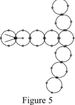
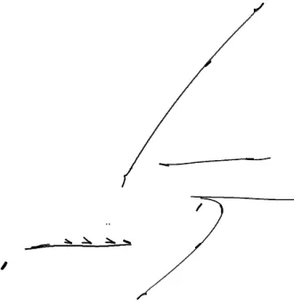
When the arrangement shown in figure 4 is simulated, the output from the 'Not' node activates the 'Thrust' node, which exerts a force on itself. This force ultimately gets transmitted along all of the nodes in the structure to which the 'Thrust' node belongs, and so the whole structure moves towards the right and collides with the vertical line of 'Insulator' nodes. Figure 5 shows this happening.
Figure 5
The vertical line of 'Insulator' nodes is pushed aside and comes to rest. Figure 6 shows the result.
Figure 6
Output
Input
A Concise Description of NODES
In NODES, time is discrete, and moves forward in steps of 1 unit. At a given instant of time, a single isolated 'Insulator' node can be described by its position, orientation, velocity and angular velocity. Every node has a mass of 1 unit and a moment of inertia of 1 unit.
All nodes in the universe experience a frictional force proportional to their velocity, and an angular frictional force proportional to their angular velocity.
Nodes have a radius of 1 unit and there is a repulsive force between any pair of overlapping nodes.
Nodes can be connected to other nodes. When two nodes are connected, they exert forces on each other in such a way as to bring themselves into proximity and alignment. Every node has four terminals evenly spaced around its edge which can be used to make connections with the terminals of other nodes. A line of connected nodes is called a filament.
Node Types and Signals
Three node types have already been introduced – these were the 'Insulator', 'Not' and 'Thrust' types. Signals were mentioned in the informal descriptions of these types.
The terminals which are used to connect nodes together are also used as inputs and outputs for passing signals between nodes. Nodes do not need to be connected in order for signals to pass between them. If an output terminal is near an input terminal, then any signal it is outputting will be received by the input terminal. Each terminal is either an input or an output. If a terminal has no explicit definition, it is effectively an output producing no signal.
Signals are 32-bit integer values. The absence of a signal corresponds to a value of zero.
A node's type determines how it responds to input signals, and whether it produces any output signals.
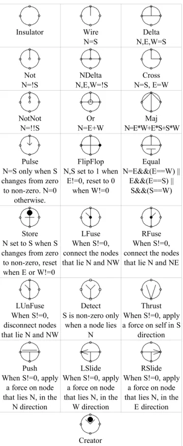
Table 2 gives an informal description of 22 commonly used node types. In table 2 the letters N,S,E and W (for North, South, East and West) are used to refer to terminals and also to indicate directions. The context should indicate which usage is meant.
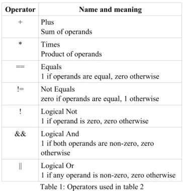
The notation used for expressions in table 2 is that used by the C programming language, summarized in table 1.
Operator Name and meaning
+ Plus
Sum of operands
* Times
Product of operands
== Equals
1 if operands are equal, zero otherwise
!= Not Equals
zero if operands are equal, 1 otherwise
! Logical Not
1 if operand is zero, zero otherwise && Logical And
1 if both operands are non-zero, zero otherwise
|| Logical Or
Insulator Wire N=S Delta N,E,W=S Not N=!S NDelta N,E,W=!S Cross N=S, E=W NotNot N=!!S Or N=E+W Maj N=E*W+E*S+S*W Pulse N=S only when S changes from zero to non-zero. N=0
otherwise.
FlipFlop N,S set to 1 when
E!=0, reset to 0 when W!=0 Equal N=E&&(E==W) || E&&(E==S) || S&&(S==W) Store N set to S when S changes from zero to non-zero, reset when E or W!=0
LFuse When S!=0, connect the nodes that lie N and NW
RFuse When S!=0, connect the nodes that lie N and NE
LUnFuse When S!=0, disconnect nodes that lie N and NW
Detect S is non-zero only
when a node lies N
Thrust When S!=0, apply a force on self in S
direction
Push When S!=0, apply
a force on node that lies N, in the
N direction
LSlide When S!=0, apply
a force on node that lies N, in the
W direction
RSlide When S!=0, apply
a force on node that lies N, in the
E direction
Creator
When S is non-zero, create a node in the N direction. The type and orientation or the new node depend on S
Table 2: Common node types
A Self Replicating Machine in NODES
The node types described in the previous section have been used to make a self replicating machine (SRM). This SRM is made from several smaller machines, which will be referred to by name. The names of these machines are: 'Instruction Tape', 'Tape Reader', 'Tape Copier', 'Dragger', 'Releaser' and 'End Finder and Reader' (EFR).
The SRM would be far more complex were it not for the 'Creator' node type. This type allows new nodes to appear from nowhere and is the least physically realistic part of the SRM.
Figure 7 shows the machine shortly after it starts. The Tape Reader is advancing along the Instruction Tape, creating a filament of nodes. Several filaments will be created, and will assemble themselves to form a 'Tape Copier', two 'End Finders and Readers' a 'Releaser' and a 'Dragger'. The Tape Copier makes a copy of the instruction tape. The Dragger takes the end of this copy, and pulls it to a new position in the universe. The Releaser disconnects the Dragger from the copy. Then, one of the 'End Finder and Reader' machines finds the end of the copy and starts the cycle again at the tape reading step. The second 'End Finder and Reader' machine does the same with the original tape. Figure 8 shows the system part way through the first replication cycle.
Figure 7: The SRM shortly after it is started. Note that only the rightmost part of the instruction tape is shown.
Figure 8:The SRM part way through the first replication cycle. The Dragger is dragging the new tape away from the original tape. The Tape Reader and the Tape Copier that worked on the original tape have finished their jobs and are outside the frame of this picture.
Instruction Tape
Tape Reader Newly created filament
EFR for original tape EFR for new tape
The following sections briefly describe the components of the self replicating machine. There is not room here for a complete description of these components. Further details can be discovered by obtaining the software required to simulate the system, details of which are given near the end of this paper.
The Instruction Tape
The instruction tape is a filament of Store nodes, the outputs of which lie along one side of the filament, as shown in figure 7.
The Tape Reader
The Tape Reader is a very simple component used only in the parent self-replicating machine. For all descendants of this parent, the function of the Tape Reader is included in the EFR components.
The job of the Tape Reader is to move along the Instruction Tape, passing the signals it encounters from the Store nodes in the Instruction Tape to a Creator node to create a sequence of nodes, which it joins together to form a filament. The Tape Reader also outputs a signal to act as a trigger to any filament that needs it.
The Tape Copier
The Tape Copier is the first component to become active after the Tape Reader has finished its task. The Tape Copier moves from its initial position towards the rightmost end of the Instruction Tape. When it touches the Instruction Tape it changes direction and begins to move along the tape, creating new Store nodes and connecting them together to make a second Instruction Tape.
Figure 9: The Tape Copier in action, copying the leftmost end of the original Instruction Tape. The V-shaped component just above Tape Copier is the Dragger, not yet fully assembled. To the right is the Releaser, assembled and waiting to be activated.
The Dragger
The Dragger is designed so that the time it takes to assemble is longer than the time taken for the Tape Copier
to finish its task. When it is active, the Dragger starts moving towards the leftmost end of the copy of the Instruction Tape. It connects itself near the end of this tape and then starts pulling it away from the original tape, as shown in figure 8. As the tape is pulled, it touches and activates the Releaser and the two EFRs.
The Releaser
After the Releaser is activated by contact with the second Instruction Tape, it proceeds to move along this tape, heading towards the Dragger. It moves very slowly, but eventually catches up with the Dragger. When the Releaser touches the Dragger, the Dragger disconnects itself from the tape.
The End Finder and Reader for the Copy
As the second Instruction Tape is dragged away from the original Instruction Tape, it brushes against this EFR. Before it is fully assembled, this component detects a signal from a Store node near the end of the Instruction Tape, and in response it connects itself to the end of this tape. It is then dragged along with the tape. When the Releaser causes the Dragger to let go of the tape, this EFR can finish assembling and then begin its task of reading the second Instruction Tape, starting another replication cycle.
The SRM in Action
Figure 10 illustrates the SRM in action. The original machine has produced three children, and is part way through making a fourth. The first child has produced a child of its own.
Figure 10: One SRM has produced several others. The separation between the SRMs has been reduced here to fit them all on the page.
Conclusion
A system has been demonstrated in which a self-replicating machine can be constructed. The laws of motion used in this system are based on Newton's laws. The particles in this system are simple, except for the 'Creator' type which can produce other particles out of nowhere. With further work, it may be possible to improve on the self replicating machine described here with respect to attributes b and e defined in the introduction.
It seems reasonable to suppose that the SRM described here can be modified so as to construct things other than copies of itself. To devise a SRM in NODES which is not dependant on the 'Creator' type seems much more challenging.
Obtaining NODES for your System
Source code, examples (including the self replicating machine described here) and a user guide for NODES are available by following the URL:
http://willsthings.mysite.freeserve.com/SRM/presentation.htm
NODES is written in C++ and has been compiled under Linux and under DOS (Using DJGPP)
References
Byl J. 1989. Self-Reproduction in small cellular automata. Physica D, Vol. 34, 295-299
Drexler K. E. 1985. Engines of Creation: The Coming Era of Nanotechnology. London: Fourth Estate.
URL: http://www.foresight.org/EOC/index.html
Freitas R. A. Jr. 1981. Report on the NASA/ASEE summer study on advanced automation for space missions. Journal of the British Interplanetary Society, Vol. 34, September 1981: 407-408.
Langton C.G. 1984. Self-reproduction in cellular automata. Physica D, Vol. 10: 135-144.
Penrose L.S. 1959. Self-reproducing machines. Scientific American, Vol. 200, No. 6: 105-114
Sayama H. 1998. Constructing Evolutionary Systems on a Simple Deterministic Cellular Automata Space. Ph. D Dissertation, Department of Information Science, Graduate School of Science, University of Tokyo.
Sipper, M. 1998. Fifty years of research on self-replication: An overview. Artificial Life, Vol. 4, No. 3: 237-257.
Sipper M. 2003. The Artificial Self-replication page. URL: http://www.cs.bgu.ac.il/~sipper/selfrep/
Tempesti G. 1995. A new self-reproducing cellular automaton capable of construction and computatioon. In F. Morán, A. Moreno, J.J. Merelo, and P. Chacón, editors, ECAL'95: Third European Conference on Artificial Life, volume 929 of Lecture Notes in Computer Science, pages 555-563, Berlin, Springer-Verlag.