Through connectivity in applied computer systems – ADMOS and MARWIN projects

(1)

Through connectivity in applied computer systems –

ADMOS and MARWIN projects

RODRIGUES, Marcos <http://orcid.org/0000-0002-6083-1303> and KORMANN, Mariza

Available from Sheffield Hallam University Research Archive (SHURA) at: http://shura.shu.ac.uk/10292/

This document is the author deposited version. You are advised to consult the publisher's version if you wish to cite from it.

Published version

RODRIGUES, Marcos and KORMANN, Mariza (2015). Through connectivity in applied computer systems – ADMOS and MARWIN projects. In: 5th Annual International Scientific Conference on Education, Science, Innovations ESI 2015, Pernik, Bulgaria, June 10-11, 2015. (Unpublished)

Copyright and re-use policy

See http://shura.shu.ac.uk/information.html

(2)

Through Connectivity in Applied Computer

Systems – ADMOS and MARWIN Projects

(3)

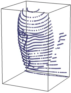
The GMPR 3D scanning technologies

3D with single image

Chapter 3 – Structured light scanning

[image:3.720.275.516.206.410.2] [image:3.720.557.680.224.384.2]

3.1 THE LAYOUT OF OUR SCANNER

Figure 3.1 illustrates the basic concept of a structured light scanner which utilizes a pattern of horizontal stripes. A projector is utilized to cast the pattern onto the surface of a target object, and a camera captures an image of the scene. Information retrieved from the image is combined with the geometric relationship between the projector and camera in order to reconstruct a cloud of points in 3D. This is possible because each stripe corresponds to a sheet of light originating from the centre of the projector lens and the image reveals where those sheets hit the target surface.

recorded image

←−

projector camera

target object

reconstructed point cloud

Figure 3.1: A series of parallel stripes is projected onto the surface of an object. A recorded image of this scene reveals the shape of the surface along those stripes, and can be used to reconstruct a 3D point cloud.

We define a Cartesian coordinate system spanning a 3D space in which the scanner is cali-brated and in which the surface can be reconstructed. Refer to Figure 3.2(a). The axes are chosen in relation to the projector such that: theX-axis coincides with the central projector

axis; the X–Y plane coincides with the horizontal sheet of light cast by the projector; and

the system origin is at an arbitrary, but fixed and known, distanceDp>0 from the centre of

the projector lens. We call the space spanned by these axes thesystem space.

29 Chapter 3 – Structured light scanning

3.1 THE LAYOUT OF OUR SCANNER

Figure 3.1 illustrates the basic concept of a structured light scanner which utilizes a pattern of horizontal stripes. A projector is utilized to cast the pattern onto the surface of a target object, and a camera captures an image of the scene. Information retrieved from the image is combined with the geometric relationship between the projector and camera in order to reconstruct a cloud of points in 3D. This is possible because each stripe corresponds to a sheet of light originating from the centre of the projector lens and the image reveals where those sheets hit the target surface.

recorded image

←−

projector camera

target object

reconstructed point cloud

Figure 3.1: A series of parallel stripes is projected onto the surface of an object. A recorded image of this scene reveals the shape of the surface along those stripes, and can be used to reconstruct a 3D point cloud.

We define a Cartesian coordinate system spanning a 3D space in which the scanner is cali-brated and in which the surface can be reconstructed. Refer to Figure 3.2(a). The axes are chosen in relation to the projector such that: theX-axis coincides with the central projector

axis; the X–Y plane coincides with the horizontal sheet of light cast by the projector; and

the system origin is at an arbitrary, but fixed and known, distanceDp>0 from the centre of

the projector lens. We call the space spanned by these axes the system space.

29

Each light plane is uniquely

(4)

The MARWIN Project

FP7 Research for the Benefit of SMEs

(5)

MARWIN: SHU work on various tasks

Marcos Rodrigues, Mariza Kormann

3D Scanner Development

Registration and fusion of 3D models

(6)

GMPR scanner design

A beam splitter allows for visible and

near-infrared cameras to be fitted

(7)

Full design integrated into a

robotic arm

(8)

(9)

Scanning a part with the robot

(10)

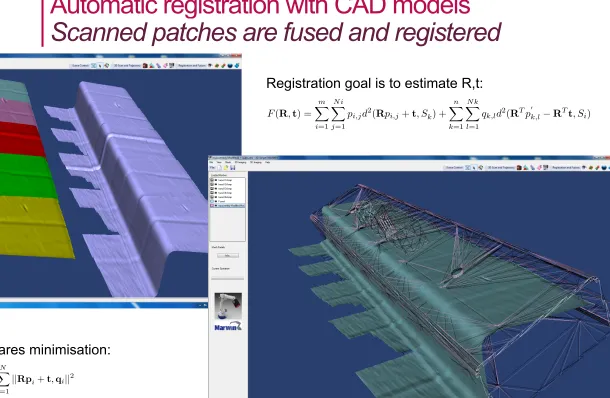
Automatic registration with CAD models

Scanned patches are fused and registered

Lecture Notes in Computer Science 7

the two sets of points pi andqi are paired to each other. The registration goal is to estimate the parameters (R,t) rotation matrix and translation vector by minimising the following objective function:

F(R,t) = m � i=1 N i � j=1

pi,jd2(Rpi,j+t, Sk) + n � k=1 N k � l=1

qk,ld2(RTp �

k,l−RTt, Si) (9)

From the objective function in (9) the distance minimisation between the two sets of points is performed in a least squares sense:

f(R,t) = 1

N

N �

i=1

||Rp_i+t,qi||2 (10)

[image:10.720.101.711.126.524.2]

When the transformation model (R,t) has been estimated, transform every point in the CAD model. This iteration is repeated until convergence to a minimum set threshold or when a predefined number of iterations is reached.

Fig. 4.Visibility constraints and registration. Top row (left and middle): model is re-oriented to display desired surface; (right): hidden surfaces are removed from a selected model. Bottom row (left): initial position; (right): after registration.

The proposed visibility constraints are necessary for partial registration, as the ICP is guaranteed to fail if one tries to register both sets of data without adequate constraints. The method is that the user will pre-orient the CAD model

Lecture Notes in Computer Science 7

the two sets of pointspi andqi are paired to each other. The registration goal is to estimate the parameters (R,t) rotation matrix and translation vector by minimising the following objective function:

F(R,t) = m � i=1 N i � j=1

pi,jd2(Rpi,j+t, Sk) + n � k=1 N k � l=1

qk,ld2(RTp �

k,l−RTt, Si) (9)

From the objective function in (9) the distance minimisation between the two sets of points is performed in a least squares sense:

f(R,t) = 1

N

�

i=1

||Rpi+t,qi||2 (10)

When the transformation model (R,t) has been estimated, transform every point in the CAD model. This iteration is repeated until convergence to a minimum set threshold or when a predefined number of iterations is reached.

Fig. 4.Visibility constraints and registration. Top row (left and middle): model is re-oriented to display desired surface; (right): hidden surfaces are removed from a selected model. Bottom row (left): initial position; (right): after registration.

The proposed visibility constraints are necessary for partial registration, as the ICP is guaranteed to fail if one tries to register both sets of data without adequate constraints. The method is that the user will pre-orient the CAD model

Registration goal is to estimate R,t:

(11)

Welding sequence

(12)

The ADMOS Project

(13)

ADMOS: SHU work on various tasks

Marcos Rodrigues, Mariza Kormann

Privacy Regulations

Modelling and System Design

Hardware and Electronics Design

Client Side Software Development: tracking, gender

and age estimation

(14)

Hardware and Electronics Design

Optics and lighting

(15)

Client Side Software Development

Firmware and control s/w development

Real time processing:

1. face detection and tracking

2. eye tracking

3. other feature tracking (mouth, nose)

4. cropping the various face-ROI

5. gender classification

6. age estimation

7. save statistical info to an xml file

(16)

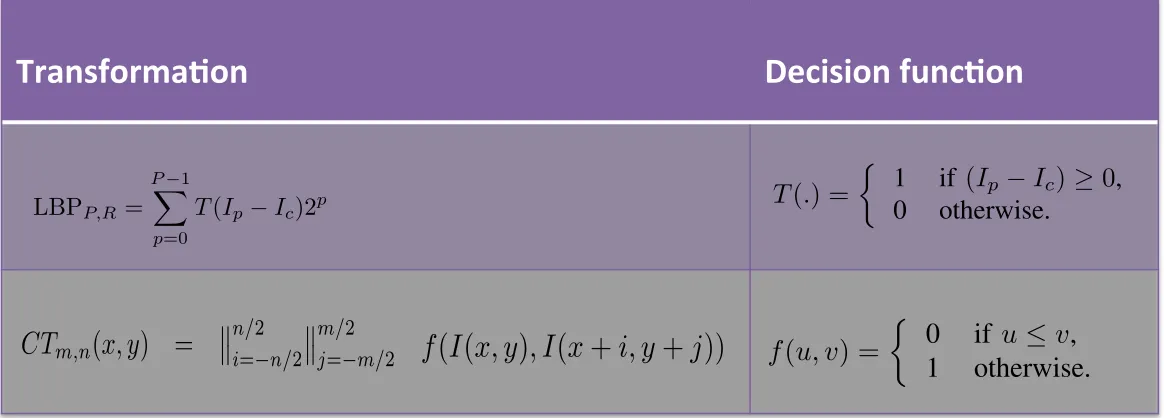
Transforma*on

Decision func*on

Binary patterns

LBP, CT and MCT

18TH INTERNATIONAL CONFERENCE ON CIRCUITS, SYSTEMS, COMMUNICATIONS AND COMPUTERS (CSCC 2014) 3

Fig. 1. The proposed method: histograms from LBP, CT and MCT are transformed by DCT. Both original histograms and their DCT are compared through SVM.

same images building training and test sets

for both classes, with kernel window size

3

×

3

;

4) Apply the discrete cosine transform to the

outputs from steps 1–3;

5) Use SVM for training and testing all data

from steps 1–4.

The proportion of data that is used for training

and testing can vary considerably; in this paper we

use 70–30 (70% of all data for training and 30%

for testing).

A. The Census Transform – CT

The Census Transform has been proposed in [14]

as a grey-level operator over a local neighbourhood.

It applies to an image kernel of size

m

×

n

:

CT

m,n

(

x, y

) =

�

n/2

i=−n/2

�

m/2

j=−m/2

(1)

f

(

I

(

x, y

)

, I

(

x

+

i, y

+

j

))

where the operator

||

is a bit-wise concatenation of

f

(

u, v

)

which is defined as

f

(

u, v

) =

�

0 if

u

≤

v

,

1 otherwise.

Various modifications have been suggested to

the original CT transform such as centre-symmetric

weighted kernel [15] and a modified CT using the

mean of the centre pixel [16]. Typical window sizes

are

3

×

3

,

5

×

5

and

9

×

7

as their concatenated binary

results fit into 8, 32 or 64 bit. Experiments have

shown (e.g. [17]) that using a kernel window of

5

×

5

is a good compromise between speed and accuracy.

The Modified Census Transform (MCT) as used

in this paper is similarly defined as in equation 1.

The difference is that instead of using the grey

level intensity of the centre pixel, the average of

the kernel window intensity is used.

B. Local Binary Patterns – LBP

Local binary patterns [2], [18], [19], [20] are

grey-scale operators defined over local

neighbour-hood pixels. It was originally defined using a

3

×

3

array of pixels, but many implementations

con-sider larger radii. The value of the centre pixel

is compared with its neighbours and the result

(greater or smaller) expressed as a binary number

and concatenated over all pixels considered. The

concatenated array of binary numbers is normally

converted to grey scale from which histograms are

produced. LBP can be expressed over

P

sampling

points on a circle of radius

R

where the value of

the centre pixel

(

x, y

)

is expressed as:

LBP

P,R

=

P

�

₋1

p=0

T

(

I

p

−

I

c

)2

p

,

(2)

where

I

p

−

I

c

is the difference of pixel intensity

in the grey level between a current pixel and centre

pixel of the kernel window.

P

is the number of

pix-els on a circle of radius

R

, and

T

is a thresholding

function defined as:

T

(

.

) =

�

1 if

(

I

p

−

I

c

)

≥

0

,

0 otherwise.

In order to improve the discriminating power

of LBPs, images are normally defined in blocks

MCT is similar to CT, except that it uses the average intensity of the kernel window as the intensity of the centre pixel.

18TH INTERNATIONAL CONFERENCE ON CIRCUITS, SYSTEMS, COMMUNICATIONS AND COMPUTERS (CSCC 2014) 3

same images building training and test sets for both classes, with kernel window size 3_×3; 4) Apply the discrete cosine transform to the

5) Use SVM for training and testing all data from steps 1–4.

The proportion of data that is used for training and testing can vary considerably; in this paper we use 70–30 (70% of all data for training and 30% for testing).

The Census Transform has been proposed in [14] as a grey-level operator over a local neighbourhood. It applies to an image kernel of size m_×n:

CTm,n(x, y) =

� �n/2

i=₋n/2 � �m/2

j=₋m/2 (1)

f(I(x, y), I(x+i, y+j))

where the operator _|| is a bit-wise concatenation of

f(u, v) which is defined as

f(u, v) =

�

0 if u_≤ v,

1 otherwise.

Various modifications have been suggested to the original CT transform such as centre-symmetric weighted kernel [15] and a modified CT using the mean of the centre pixel [16]. Typical window sizes are 3_×3, 5_×5 and 9_×7 as their concatenated binary results fit into 8, 32 or 64 bit. Experiments have shown (e.g. [17]) that using a kernel window of 5_×5 is a good compromise between speed and accuracy. The Modified Census Transform (MCT) as used in this paper is similarly defined as in equation 1. The difference is that instead of using the grey level intensity of the centre pixel, the average of the kernel window intensity is used.

B. Local Binary Patterns – LBP

Local binary patterns [2], [18], [19], [20] are grey-scale operators defined over local neighbour-hood pixels. It was originally defined using a 3_×3 array of pixels, but many implementations con-sider larger radii. The value of the centre pixel is compared with its neighbours and the result (greater or smaller) expressed as a binary number and concatenated over all pixels considered. The concatenated array of binary numbers is normally converted to grey scale from which histograms are produced. LBP can be expressed over P sampling

points on a circle of radius R where the value of

the centre pixel (x, y) is expressed as:

LBPP,R = P�−1

p=0

T(Ip −Ic)2p, (2)

where Ip − Ic is the difference of pixel intensity in the grey level between a current pixel and centre pixel of the kernel window. P is the number of

pix-els on a circle of radius R, and T is a thresholding

T(.) =

�

1 if (Ip−Ic)≥ 0, 0 otherwise.

In order to improve the discriminating power of LBPs, images are normally defined in blocks 18TH INTERNATIONAL CONFERENCE ON CIRCUITS, SYSTEMS, COMMUNICATIONS AND COMPUTERS (CSCC 2014) 2

lip detection algorithms. The method is described in Section II, experimental results are presented in Section III with a conclusion in Section IV.

II. METHOD

In order to perform real-time gender classifica-tion, a number of steps are necessary. First faces must be detected in the image and this is achieved through the Viola-Jones method [10], [11] available from OpenCV libraries. An unconstrained image may contain a number of faces and each region of interest ROI containing a face must be processed independently and the detected gender must be assigned to a corresponding data structure (to that region of interest). The data structure thus, will contain a gender attribute such that to avoid un-necessary multiple calls to the gender classification function if a particular tracked face has already a gender definition. This applies to the tracking of faces over multiple frames, but these aspects are not discussed further in this paper. Instead the focus is on sensitivity analysis over selected regions of the face.

Sensitivity analysis starts with testing aspect ratios of the ROI concerning the selected facial region. The Viola-Jones method yields a ROI with aspect ratio of 1 : 1. The method, however, suffers

from false positive detection: due to the simplicity of the Haar-like features used, some of the detected face objects are not faces at all. In order to verify whether or not it is a face, a number of constraints are imposed namely, a face must have two eyes and a lip. To verify the constraints each ROI is taken in turn. First eye detection is performed in the knowledge that right and left eyes are located in the first and second quadrants of the ROI, and lip detection in the knowledge that the lip is spread over the third and fourth quadrants. An example of a verified face is depicted in Figure 1. If the ROI satisfies these constraints then proceed to gender classification. Note that eye detection is a specific requirement of the ADMOS project but very useful in the context of sensitivity analysis presented here as the size of a larger ROI (of aspect ratio of 3:4) is determined from the eye locations.

Fig. 1. Face, eyes, and lip detection in real time with annotated face ROI of aspect ratio1 : 1

Local binary patterns [2], [4] are grey-scale operators useful for texture classification defined over local neighbourhood pixels. It was originally defined using a 3_×3 array of pixels. The value of

the centre pixel is compared with its neighbours and the result (greater or smaller) expressed as a binary number and summed over all pixels considered. LBP can be expressed over P sampling points on a circle of radius R where the value of the centre pixel (x, y) is expressed as:

LBPP,R = P�−1

p=0

T(Ip−Ic)2p, (1)

where Ip and Ic refer to the pixel intensity in the

grey level of the centre pixel and of P pixels on a circle of radiusR, andT is a thresholding function with T(.) = 1 if (Ip − Ic) ≥ 0 or T(.) = 0

otherwise. Normally images are defined in blocks from which individual LBPs are calculated and then concatenated into a single histogram. The analysis of such histograms can be used to differentiate tex-ture patterns. The size of the block under analysis can vary and this obviously will be reflected in the LBP histogram.

In order to improve the robustness and

discrimi-18TH INTERNATIONAL CONFERENCE ON CIRCUITS, SYSTEMS, COMMUNICATIONS AND COMPUTERS (CSCC 2014) 3

same images building training and test sets

3

×

3

;

from steps 1–4.

and testing can vary considerably; in this paper we

for testing).

m

×

n

:

CTm,n

(

x, y

) =

�

n/_i₌2₋_n/₂

�

m/_j₌₋2_m/₂

(1)

f

(

I

(

x, y

)

, I

(

x

+

i, y

+

j

))

where the operator

||

is a bit-wise concatenation of

f

(

u, v

)

which is defined as

f

(

u, v

) =

�

0 if

u

≤

v

,

1 otherwise.

are

3

×

3

,

5

×

5

and

9

×

7

results fit into 8, 32 or 64 bit. Experiments have

shown (e.g. [17]) that using a kernel window of

5

×

5

the kernel window intensity is used.

B. Local Binary Patterns – LBP

3

×

3

is compared with its neighbours and the result

(greater or smaller) expressed as a binary number

P

sampling

R

where the value of

the centre pixel

(

x, y

)

is expressed as:

LBP

P,R

=

P

�

−1

p=0

T

(

Ip

−

Ic

)2

p

,

(2)

where

Ip

−

Ic

P

is the number of

R

, and

T

is a thresholding

T

(

.

) =

�

1 if

(

Ip

−

Ic

)

≥

0

,

0 otherwise.

In order to improve the discriminating power

of LBPs, images are normally defined in blocks

18TH INTERNATIONAL CONFERENCE ON CIRCUITS, SYSTEMS, COMMUNICATIONS AND COMPUTERS (CSCC 2014) 3

same images building training and test sets

3

×

3;

from steps 1–4.

and testing can vary considerably; in this paper we

for testing).

m

×

n

:

CT

m,n

(

x, y

) =

�

n/2

i=₋n/2

�

m/2

j=₋m/2

(1)

f

(

I

(

x, y

)

, I

(

x

+

i, y

+

j

))

where the operator

||

is a bit-wise concatenation of

f

(

u, v

)

which is defined as

f

(

u, v

) =

�

0 if

u

≤

v

,

1 otherwise.

are

3

×

3,

5

×

5

and

9

×

7

results fit into 8, 32 or 64 bit. Experiments have

shown (e.g. [17]) that using a kernel window of

5

×

5

the kernel window intensity is used.

B. Local Binary Patterns – LBP

3

×

3

is compared with its neighbours and the result

(greater or smaller) expressed as a binary number

P

sampling

R

where the value of

the centre pixel

(

x, y

)

is expressed as:

LBP

P,R

=

P

�

−1

p=0

T

(

I

p

−

I

c

)2

p

,

(2)

where

I

p

−

I

c

P

is the number of

R

, and

T

is a thresholding

T

(

.

) =

�

1 if

(

I

p

−

I

c

)

≥

0,

0 otherwise.

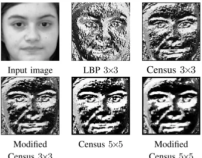
[image:16.720.70.652.222.431.2]

(17)

Applying binary patterns to face images

Visualizing the differences on images

18TH INTERNATIONAL CONFERENCE ON CIRCUITS, SYSTEMS, COMMUNICATIONS AND COMPUTERS (CSCC 2014)

5

Fig. 2. Examples of image data from the FEI database.

Input image

LBP

3

×

3

Census

3

×

3

Modified

Census

5

×

5

Modified

Census

3

×

3

Census

5

×

5

Fig. 3. LBP, Census and Modified Census over an input image.

and this is left for further studies. Here we report

on LBP, CT and MCT with constant

3

×

3

kernel

window.

Following results described in [13] we use the

face regions labeled as FULL face, TOP and

BOT-TOM half of the face. Histograms for LBP, CT

and MCT were evaluated as described in

Sec-tion II. From these we also built concatenated

histograms for FULL

||

TOP, FULL

||

BOTTOM, and

TOP

||

BOTTOM. Furthermore, we also built

con-catenated histograms of LBP

||

CT and LBP

||

MCT

for all cases. The histograms were then separated

into training and test sets and subject to the SVM

discrimination method.

TABLE I

A

CCURACY OF HISTOGRAM

-

BASED CLASSIFICATION

(%)

Face ROI &

LBP

||

LBP

||

Method

LBP

CT

MCT

CT

MCT

FULL

Female

80.6

87.1

67.7

83.9

77.4

Male

90.3

93.5

83.9

90.3

83.9

TOP

Female

83.9

87.1

74.7

83.9

80.6

Male

96.8

87.1

77.4

90.3

BOTTOM

Female

80.6

74.2

67.7

71.0

74.2

Male

93.5

96.8

93.5

FULL

||

TOP

Female

83.4

87.1

77.4

87.1

Male

93.5

87.1

96.8

87.1

FULL

||

BOTTOM

Female

83.9

87.1

64.5

71.0

77.4

Male

90.3

93.5

90.3

96.8

TOP

||

BOTTOM

Female

80.6

67.7

74.2

83.9

80.6

Male

96.8

100.0

90.3

93.5

Mean

87.9

87.6

79.0

86.3

85.2

STD

6.4

8.9

9.9

9.4

7.3

Mean Female

82.2

81.7

71.0

78.5

79.6

Mean Male

93.5

87.1

94.1

90.9

Abs difference

11.4

11.8

16.1

15.6

11.3

Results for histogram-based classification are

tab-ulated in Table I. The summary refers to training

on 60 data sets (30 female, 30 male) and 60 test

sets. The best result is for LBP applied to the TOP

half of the face, and this confirms previous results

as reported in [13]. Overall, the LBP technique

is shown to be superior to CT and MCT and the

concatenated combinations with the overall lowest

standard deviation of 6.4. Furthermore, it is

ob-served that there is a bias towards more accurate

male classification as reported in all papers in the

literature; this is the case for all combinations used.

The reasons for this behaviour are not yet clear.

[image:17.720.163.568.200.517.2]

(18)

LBP processing

(19)

ROI sensitivity analysis

Male subjects tend to be

classified with higher

accuracy.

This agrees with all results

reported in the literature.

No explanation for this

behaviour is offered at this

stage.

18TH INTERNATIONAL CONFERENCE ON CIRCUITS, SYSTEMS, COMMUNICATIONS AND COMPUTERS (CSCC 2014) 5

TABLE I

COMPARATIVE ANALYSIS OF IMAGE REGIONS

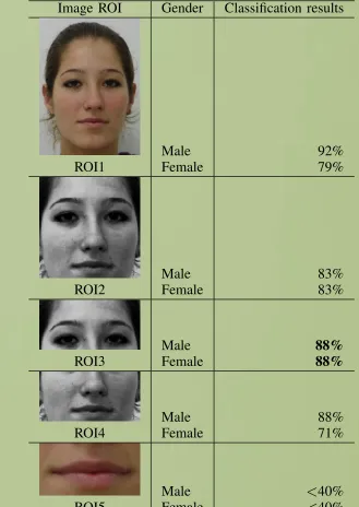
Image ROI Gender Classification results

Male 92%

ROI1 Female 79%

Male 83%

ROI2 Female 83%

Male 88%

ROI3 Female 88%

Male 88%

ROI4 Female 71%

Male <40%

ROI5 Female <40%

to detect both classes with good accuracy. ROI4

(consisting of the bottom half of ROI2) retained its

previous accuracy for male subjects at 88% but for

female the performance decreased substantially to

71%. This shows that the region does not contain

enough variation in texture to guarantee robust

classification, which is somewhat surprising. Before

testing this ROI, it was expected that, due to facial

hair and skin texture variations on either shaved and

unshaved faces, male and female subjects would be

detected with the highest degree of accuracy. Finally

ROI5 has proved to be problematic as automatic lip

detection failed in about half of the data (multiple

lip detection was deemed a failure). Thus the lack

of robust lip detection rendered this ROI unstable

and the statistics reported here at less than 40% are

just an indication of performance.

Since this research is only interested in the

minimum ROI with highest performance, results

demonstrate that ROI3 is the most promising one.

The high variance caused by skin texture, eyebrows,

eyes, and portions of hair mean that the region can

be further exploited for more robust classification.

With this information, it is now possible to focus

on improvements to LBP and to the classification

algorithms. The obvious avenues to explore include

the use the Fisher’s criterion and SVM-support

vec-tor machines. In particular, SVM holds the highest

promise as it is a technique designed to maximising

the margin between canonical hyperplanes

sepa-rating the two classes. With a higher margin, the

probability of misclassification naturally decreases

and it should be possible to achieve higher accuracy

for both male and female subjects.

IV. C

ONCLUSION

This paper has presented a sensitivity analysis of

gender classification based on LBP and

eigenvec-tor decomposition over 5 regions of interest. The

adopted methodology was directed towards testing

the LBP algorithm over the selected regions to

determine the smaller region of interest yielding

the best classification results. Images from a public

database were used on which automatic detection

of the face region, eyes, and lips were performed

resulting in the various regions of interest being

defined. Classification results show that the region

containing parts of the nose, eyes and front are the

most reliable, with an overall accuracy of 88% for

both male and female subjects.

[image:19.720.331.660.61.525.2]

(20)

Comparative analysis of binary patterns

DCT-Discrete Cosine Transform

The length of coefficients

y

is the same size as the original signal

z

.

18TH INTERNATIONAL CONFERENCE ON CIRCUITS, SYSTEMS, COMMUNICATIONS AND COMPUTERS (CSCC 2014) 4

from which individual LBPs are calculated and then

concatenated into a single histogram. The analysis

of such histograms can be used to differentiate

texture patterns. A number of variants to LBP have

been proposed in the literature (e.g. [3], [4], [5]).

In the experiments reported in this paper we only

consider the original LBP definition.

C. The Discrete Cosine Transform – DCT

The DCT transform and its variants have been

used in a number of contexts most notably in image

and video compression (e.g. [21], [22], [23]). DCT

is a close relative to the discrete Fourier transform

as it defines a sequence of data in terms of the

sum of the cosine functions at different frequencies.

There are many versions of the DCT and here

we use the unitary discrete cosine transform as

defined in Matlab [24]. The DCT transform of a

one-dimensional signal

z

(in our case

z

is an image

histogram) is expressed as:

y

(

k

) =

w

(

k

)

N

�

n=1

z

(

n

) cos(

π

(2

n

−

1)(

k

−

1)

2

N

)

(3)

for

k

= 1

,

2

, . . . N

where

N

is the length of the

signal and

w

(

k

) =

�

1

/

√

N

for

k

= 1

,

�

2

/N

for

2

≤

k

≤

N .

(4)

The length of the coefficients

y

is the same as

the original signal

z

. A useful property of the

DCT is that normally it is only necessary a few

coefficients to reconstruct the signal; most signals

can be described with over 99% accuracy by using

only a handful of coefficients. Here we choose to

use all coefficients for improved accuracy.

D. Support Vector Machines – SVM

In pattern recognition tasks, algorithms for linear

discriminant functions can be used either over the

raw or original data features or in a transformed

space that can be defined by nonlinear

transforma-tions of the original variables (e.g. DCT applied

to the LBP and CT histograms as proposed in

this paper). Support vector machines are algorithms

that implement a mapping of pattern vectors to a

higher dimensional feature space and find a ‘best’

separating hyperplane between the data set. The

best hyperplane is commonly referred to as the

maximal margin hyperplane, as it is defined where

the closest points between classes are at maximum

distance [25].

Given a set of

M

training samples (

l

i

,

x

i

) where

l

_i

is the associated class label (

l

_i

∈

{−

1

,

1

}

) of

vector

x

_i

where

x

_i

∈

R

N

, a SVM classifier finds

the optimal hyperplane that maximises the margin

between classes

l

i

:

f

(

x

) =

M

�

i=1

l

_i

α

_i

·

k

(

x

,

x

_i

) +

b

(5)

where

k

(

x

,

x

_i

)

is a kernel function,

b

is a bias and

the sign of

f

(

x

)

is used to determine the class

membership of vector

x

. For a two-class problem

(e.g. the case of gender classification) a linear SVM

might suffice. In this case, the kernel function is a

dot product in the input space.

III. E

XPERIMENTAL RESULTS

A public database as described in [13] is used

here, details of the database can be found in [26].

It contains 2,779 images of even balanced number

of male and female subjects captured with large

variations in pose and illumination. In [13] a set of

50 male and 50 female subjects were used; although

all subjects were not in strictly frontal pose, there

was not much variation in illumination in that

dataset. Here we expand the dataset by including

images with uneven illumination. We used the entire

set of 99 male and 99 female subjects (one subject

was removed from each original set of 100 as they

appear to be repeated). The selected data allows

the testing of algorithms in a realistic scenario of

uneven illumination. Examples of selected images

from the database are depicted in Figure 2.

First, we performed a visual comparison of LBP,

CT and MCT using a

3

×

3

kernel window. We

proceeded to perform a CT and MCT using a

5

×

5

window as shown in Figure 3. It is not clear

whether or not simply increasing the kernel size

would impact on gender classification performance

18TH INTERNATIONAL CONFERENCE ON CIRCUITS, SYSTEMS, COMMUNICATIONS AND COMPUTERS (CSCC 2014) 4

from which individual LBPs are calculated and then

concatenated into a single histogram. The analysis

C. The Discrete Cosine Transform – DCT

The DCT transform and its variants have been

There are many versions of the DCT and here

we use the unitary discrete cosine transform as

z

(in our case

z

is an image

y

(

k

) =

w

(

k

)

N

�

n=1

z

(

n

) cos(

π

(2

n

−

1)(

k

−

1)

2

N

)

(3)

for

k

= 1

,

2

, . . . N

where

N

signal and

w

(

k

) =

�

1

/

√

N

for

k

= 1

,

�

2

/N

for

2

≤

k

≤

N .

(4)

y

is the same as

the original signal

z

DCT is that normally it is only necessary a few

D. Support Vector Machines – SVM

discriminant functions can be used either over the

this paper). Support vector machines are algorithms

higher dimensional feature space and find a ‘best’

distance [25].

Given a set of

M

training samples (

l

i

,

x

i

) where

l

i

l

i

∈

{−

1

,

1

}

) of

vector

x

i

where

x

i

∈

R

N

between classes

l

i

:

f

(

x

) =

M

�

i=1

l

i

αi

·

k

(

x

,

x

i

) +

b

(5)

where

k

(

x

,

x

i

)

b

is a bias and

the sign of

f

(

x

)

membership of vector

x

. For a two-class problem

might suffice. In this case, the kernel function is a

III. E

XPERIMENTAL RESULTS

of male and female subjects captured with large

50 male and 50 female subjects were used; although

images with uneven illumination. We used the entire

was removed from each original set of 100 as they

First, we performed a visual comparison of LBP,

CT and MCT using a

3

×

3

kernel window. We

proceeded to perform a CT and MCT using a

5

×

5

18TH INTERNATIONAL CONFERENCE ON CIRCUITS, SYSTEMS, COMMUNICATIONS AND COMPUTERS (CSCC 2014) 4

from which individual LBPs are calculated and then

concatenated into a single histogram. The analysis

C. The Discrete Cosine Transform – DCT

The DCT transform and its variants have been

There are many versions of the DCT and here

we use the unitary discrete cosine transform as

z

(in our case

z

is an image

y

(

k

) =

w

(

k

)

N

�

n=1

z

(

n

) cos(

π

(2

n

−

1)(

k

−

1)

2

N

)

(3)

for

k

= 1

,

2

, . . . N

where

N

signal and

w

(

k

) =

�

1

/

√

N

for

k

= 1

,

�

2

/N

for

2

≤

k

≤

N .

(4)

y

is the same as

the original signal

z

DCT is that normally it is only necessary a few

D. Support Vector Machines – SVM

discriminant functions can be used either over the

this paper). Support vector machines are algorithms

higher dimensional feature space and find a ‘best’

distance [25].

Given a set of

M

training samples (

l

i

,

x

i

) where

l

i

l

i

∈

{

−

1

,

1

}

) of

vector

x

i

where

x

i

∈

R

N

between classes

l

i

:

f

(

x

) =

M

�

i=1

l

i

α

i

·

k

(

x

,

x

i

) +

b

(5)

where

k

(

x

,

x

i

)

b

is a bias and

the sign of

f

(

x

)

membership of vector

x. For a two-class problem

might suffice. In this case, the kernel function is a

III. E

XPERIMENTAL RESULTS

of male and female subjects captured with large

50 male and 50 female subjects were used; although

images with uneven illumination. We used the entire

was removed from each original set of 100 as they

First, we performed a visual comparison of LBP,

CT and MCT using a

3

×

3

kernel window. We

proceeded to perform a CT and MCT using a

5

×

5

Decomposes a signal and defines it as a

(21)

Comparative analysis of binary patterns

DWT-Discrete Wavelet Transform

2.4 The Discrete Wavelet Transform – DWT

The DWT transform [17, 41, 42, 43] is a time-scale representation of a signal obtained using digital filtering techniques in which the signal to be analysed is passed through filters with different cutoff frequencies at different scales. The technique is realised by iteration and the resolution of the signal which determines the amount of information in the signal can be controlled by subsampling (up and down) operations. For a given signal two sets of coefficients are computed referred to as theapproximation coefficientsA

and detail coefficientsD. The A coefficients are obtained by convolving the signal with a low-pass filter and the D are obtained

by convolving with a high-pass filter.

As the signal is decomposed by the half band filters this results in signals spanning only half the frequency band. This doubling of frequency resolution reduces uncertainty in frequency by half. Following Nyquist’s rule the signal can now be down sampled by discarding half the samples with no loss of information. The result is that while the half band low pass filtering removes half the frequencies thus halving the resolution, a decimation by 2 halves the time resolution and thus doubles the scale.

Convolving the signalz(n)with a half band digital low pass filter with impulse response h(n)can be defined in discrete time

as [44]:

x(n)h(n) = ∞ �

k=_−∞

x(k)h(n₋k) (5)

Applying the Nyquist rule by subsampling the signal by 2 can be represented as

y(n) = ∞ �

k=−∞

h(k) x(2n₋k) (6)

Equation 6 is used for both high pass and low pass filtering operations. This one level decomposition can be expressed as:

yhigh =

�

n

x(n)g(2k₋n) (7)

ylow =

�

n

x(n)h(2k₋n) (8)

where yhigh and ylow are the outputs of high and low pass filters after decimation by 2. In order to reconstruct the original signal the procedure is straightforward given that half-band filters form orthonormal bases. At every level of decomposition the signal is up sampled by two, filtered through high pass and low pass synthesis filters g�(n)and h�(n) and then summed over. Thus, for

every level of decomposition the recovered signal is represented as:

x(n) = ∞ �

k=_−∞

(yhigh(k).g(−n+ 2k)) (ylow(k).h(−n+ 2k)) (9)

It is important to note that if the filters are not ideal half band, then perfect reconstruction is not possible. While it is clear that ideal filters are not possible to realise, some filters under some conditions can provide perfect reconstruction. The most used and accurate ones are the Daubechie’s filters also known as Daubechies wavelets [42] and these are the ones used in the experimental results described in Section 4.

2.5 Eigenvector Decomposition

The set of measures for gender classification is defined by the histogram produced as a result of applying LBP/CT/MCT to the image ROI. It subsumes a large number of variables and the purpose is to identify which ones are more relevant to the problem at hand. Here the problem is approached by analysis of variance, or principal values. There are at least three ways a set of principal components can be derived [20]. Ifmi is the set of original variables, then they can be expressed as a linear combination ψ:

ψi = p �

j=1

aijmj (10)

The Hotelling approach as described in [20] is used in which the purpose is to find a linear separation for which the sum of the squares of perpendicular distances is a maximum, that is, the choice is to maximise the variance ofψ. This is a common approach to the problem based on first determining the scatter matrix S by subtracting all values from their mean. Then the covariance

matrix is estimated asΣ = SST_{. The principal components are determined by performing an eigenvector decomposition of the}

symmetric positive definite matrixΣand then using the eigenvalues as coefficients in a linear combination of the original variables

m.

In order to determine class membership, the method is to define a training set in which ground truth representative of male and female images are used and classified accordingly. The leave-one-out technique can be used at testing stage if the number of samples is small. The principle is that the closest vector in the database real class is the proposed class for the testing vector.

2.4 The Discrete Wavelet Transform – DWT

The DWT transform [17, 41, 42, 43] is a time-scale representation of a signal obtained using digital filtering techniques in which

the signal to be analysed is passed through filters with different cutoff frequencies at different scales. The technique is realised by

iteration and the resolution of the signal which determines the amount of information in the signal can be controlled by subsampling

(up and down) operations. For a given signal two sets of coefficients are computed referred to as the

approximation coefficients

A

and

detail coefficients

D

. The

A

coefficients are obtained by convolving the signal with a low-pass filter and the

D

are obtained

As the signal is decomposed by the half band filters this results in signals spanning only half the frequency band. This doubling

of frequency resolution reduces uncertainty in frequency by half. Following Nyquist’s rule the signal can now be down sampled

by discarding half the samples with no loss of information. The result is that while the half band low pass filtering removes half

the frequencies thus halving the resolution, a decimation by 2 halves the time resolution and thus doubles the scale.

Convolving the signal

z

(

n

)

with a half band digital low pass filter with impulse response

h

(

n

)

can be defined in discrete time

as [44]:

x

(

n

)

h

(

n

) =

∞

�

k=−∞

x

(

k

)

h

(

n

−

k

)

(5)

y

(

n

) =

∞

�

k=−∞

h

(

k

)

x

(2

n

−

k

)

(6)

y

high

=

�

n

x

(

n

)

g

(2

k

−

n

)

(7)

y

low

=

�

n

x

(

n

)

h

(2

k

−

n

)

(8)

where

y

high

and

y

low

are the outputs of high and low pass filters after decimation by 2. In order to reconstruct the original signal

the procedure is straightforward given that half-band filters form orthonormal bases. At every level of decomposition the signal

is up sampled by two, filtered through high pass and low pass synthesis filters

g

�

(

n

)

and

h

�

(

n

)

and then summed over. Thus, for

x

(

n

) =

∞

�

k=−∞

(

y

high

(

k

)

.g

(

−

n

+ 2

k

)) (

y

low

(

k

)

.h

(

−

n

+ 2

k

))

(9)

It is important to note that if the filters are not ideal half band, then perfect reconstruction is not possible. While it is clear that

ideal filters are not possible to realise, some filters under some conditions can provide perfect reconstruction. The most used and

accurate ones are the Daubechie’s filters also known as Daubechies wavelets [42] and these are the ones used in the experimental

results described in Section 4.

2.5 Eigenvector Decomposition

The set of measures for gender classification is defined by the histogram produced as a result of applying LBP/CT/MCT to the

image ROI. It subsumes a large number of variables and the purpose is to identify which ones are more relevant to the problem at

hand. Here the problem is approached by analysis of variance, or principal values. There are at least three ways a set of principal

components can be derived [20]. If

m

i

is the set of original variables, then they can be expressed as a linear combination

ψ

:

ψ

i

=

p

�

j=1

a

ij

m

j

(10)

The Hotelling approach as described in [20] is used in which the purpose is to find a linear separation for which the sum of the

squares of perpendicular distances is a maximum, that is, the choice is to maximise the variance of

ψ

. This is a common approach

to the problem based on first determining the scatter matrix

S

by subtracting all values from their mean. Then the covariance

matrix is estimated as

Σ

=

SS

T

. The principal components are determined by performing an eigenvector decomposition of the

symmetric positive definite matrix

Σ

and then using the eigenvalues as coefficients in a linear combination of the original variables

m

.

In order to determine class membership, the method is to define a training set in which ground truth representative of male

and female images are used and classified accordingly. The leave-one-out technique can be used at testing stage if the number of

samples is small. The principle is that the closest vector in the database real class is the proposed class for the testing vector.

2.4 The Discrete Wavelet Transform – DWT

and detail coefficientsD. The Acoefficients are obtained by convolving the signal with a low-pass filter and the D are obtained

Convolving the signalz(n)with a half band digital low pass filter with impulse responseh(n)can be defined in discrete time

as [44]:

x(n)h(n) =

∞

�

k=−∞

x(k)h(n−k) (5)

y(n) =

∞

�

k=−∞

h(k)x(2n₋k) (6)

yhigh =

�

n

x(n)g(2k₋n) (7)

ylow =

�

n

x(n)h(2k−n) (8)

whereyhigh and yloware the outputs of high and low pass filters after decimation by 2. In order to reconstruct the original signal

the procedure is straightforward given that half-band filters form orthonormal bases. At every level of decomposition the signal is up sampled by two, filtered through high pass and low pass synthesis filtersg�(n)andh�(n)and then summed over. Thus, for

x(n) =

∞

�

k=−∞

2.5 Eigenvector Decomposition

The set of measures for gender classification is defined by the histogram produced as a result of applying LBP/CT/MCT to the image ROI. It subsumes a large number of variables and the purpose is to identify which ones are more relevant to the problem at hand. Here the problem is approached by analysis of variance, or principal values. There are at least three ways a set of principal components can be derived [20]. Ifmi is the set of original variables, then they can be expressed as a linear combinationψ:

ψi = p

�

j=1

aijmj (10)

The Hotelling approach as described in [20] is used in which the purpose is to find a linear separation for which the sum of the squares of perpendicular distances is a maximum, that is, the choice is to maximise the variance ofψ. This is a common approach

to the problem based on first determining the scatter matrix S by subtracting all values from their mean. Then the covariance

matrix is estimated asΣ = SST. The principal components are determined by performing an eigenvector decomposition of the

m.

In order to determine class membership, the method is to define a training set in which ground truth representative of male and female images are used and classified accordingly. The leave-one-out technique can be used at testing stage if the number of samples is small. The principle is that the closest vector in the database real class is the proposed class for the testing vector.

2.4 The Discrete Wavelet Transform – DWT

anddetail coefficientsD. The Acoefficients are obtained by convolving the signal with a low-pass filter and theD are obtained

Convolving the signalz(n)with a half band digital low pass filter with impulse responseh(n)can be defined in discrete time

as [44]:

x(n)h(n) =

∞

�

k=_−∞

x(k)h(n₋k) (5)

y(n) =

∞

�

k=−∞

h(k)x(2n₋k) (6)

yhigh =

�

n

x(n)g(2k₋n) (7)

ylow =

�

n

x(n)h(2k₋n) (8)

whereyhigh and ylow are the outputs of high and low pass filters after decimation by 2. In order to reconstruct the original signal

the procedure is straightforward given that half-band filters form orthonormal bases. At every level of decomposition the signal is up sampled by two, filtered through high pass and low pass synthesis filtersg�(n)andh�(n)and then summed over. Thus, for

x(n) =

∞

�

k=_−∞

2.5 Eigenvector Decomposition

The set of measures for gender classification is defined by the histogram produced as a result of applying LBP/CT/MCT to the image ROI. It subsumes a large number of variables and the purpose is to identify which ones are more relevant to the problem at hand. Here the problem is approached by analysis of variance, or principal values. There are at least three ways a set of principal components can be derived [20]. Ifmiis the set of original variables, then they can be expressed as a linear combinationψ:

ψi = p

�

j=1

aijmj (10)

The Hotelling approach as described in [20] is used in which the purpose is to find a linear separation for which the sum of the squares of perpendicular distances is a maximum, that is, the choice is to maximise the variance ofψ. This is a common approach

to the problem based on first determining the scatter matrix S by subtracting all values from their mean. Then the covariance

matrix is estimated asΣ = SST. The principal components are determined by performing an eigenvector decomposition of the

m.

(22)

Comparative analysis

of binary patterns

Raw histograms

(23)

Tested on public databases

(24)

Classification results

(25)

Real time and privacy requirements

(26)

Conclusions

LBP + Eigenvector decomposition: top half of the face most significant Binary patterns + SVM: LBP is slightly superior to CT/MCT

Binary patterns + DCT + SVM: CT is clearly the superior technique Also, bias towards male subjects is removed

CT has the smallest standard deviation of all techniques Real-time performance: enabled by multiple threads using multi-level queues

http://shura.shu.ac.uk/information.html

http://shura.shu.ac.uk