Formal Methods and Tools Faculty of EEMCS
Master of Science Thesis
Quiescent
Transition Systems
Author:
Gerjan
Stokkink
, B.Sc.
Examination Committee:
Mw.dr. Mari¨
elle
Stoelinga
Mark
Timmer
, M.Sc.
Prof.dr.ir. Arend
Rensink
People talking without speaking People hearing without listening
People writing songs that voices never share And no one dared
Disturb the sound of silence
Abstract
Quiescence is a fundamental concept in modelling system behaviour, as it explicitly represents the fact that, in certain system states, no output is provided by the system. The notion of quiescence is also essential to model-based testing: if a particular implementation under test does not provide any output, then the test evaluation algorithm must decide whether to allow this behaviour, or not. A Suspension Automaton (SA) is a kind of labelled transition system in which observations of quiescence are explicitly represented with specialδ-transitions. SAs form the basic building block on which the well-knowniocomodel-based testing framework is based.
The SA model, however, has a number of flaws. First of all, a SA is not defined as an entity in itself, and cannot be built from scratch. Secondly, its properties have not been fully investigated yet. Thirdly, and most importantly, the SA model does not allow nondeterminism or divergence to occur, thereby limiting the number of systems that can be naturally modelled. To address these limitations, we introduce in this thesis the so-called Quiescent Transition Systems (QTSs), which form a fully formalised alternative to the existing SAs. We also introduce Divergent Quiescent Transition Systems (DQTSs), a more complex variant on QTSs which allow (state-finite) divergence to occur.
Acknowledgements
I would like to extend my sincere gratitude to my supervisors Mari¨elle, Mark and Arend, who have guided me patiently throughout the long process of writing this thesis with their sound advice, useful comments, and in particular their motivational support. Without their efforts I would never have been able to finish this thesis in time. In particular I would like to thank Mark for his outstanding work in reviewing every chapter of this thesis, some many times over, and his invaluable help with finishing some of the more complex proofs.
I would also like to thank my parents and sisters, for always being there for me. When the going got tough they were always there to support me. I am also very grateful to my student counsellor, Renate, who helped me tirelessly with many DUO-related issues. Many thanks also to Gijs for proofreading my thesis one last time.
Finally, the process of writing this thesis would have been far less enjoyable without the camaraderie of my colleagues in the Labruimte FMT and the many friends I made within the FMT group. In particular, I would like to thank (in no particular order) Tom, Marina, Lesley, Freark, Harold, Ronald, Vincent, Maarten, Jaco, Stefano, Stefan, and Axel, amongst many others. The fun times and lively discussions I have had with you all certainly made me feel at home at all times.
Table of Contents
1 Introduction 1
2 Background 5
2.1 Notational Preliminaries . . . 5
2.2 Labelled Transition Systems . . . 6
2.2.1 The LTS Model . . . 6
2.2.2 Operations . . . 8
2.3 Input-Output Transition Systems . . . 10
2.3.1 The IOTS Model . . . 11
2.3.2 Operations . . . 12
2.4 Input-Output Automata . . . 12
2.4.1 The IOA Model . . . 13
2.4.2 Operations . . . 15
2.5 Suspension Automata . . . 16
2.6 Summary . . . 17
3 Quiescent Transition Systems 19 3.1 The QTS Model . . . 19
3.2 Well-formedness . . . 21
3.3 Deltafication: from IOTS to QTS . . . 22
3.4 Operations . . . 24
3.4.1 Parallel Composition . . . 24
3.4.2 Action Hiding . . . 25
3.5 Properties . . . 25
3.5.1 Closure Properties . . . 25
3.5.2 Commutativity Properties . . . 30
3.6 Discussion of the Well-formedness Rules . . . 33
3.6.1 Rationale behind the Well-formedness Rules . . . 33
3.6.2 Alternatives to the Well-formedness Rules . . . 36
3.7 Summary . . . 37
4 Divergent Quiescent Transition Systems 39 4.1 The DQTS Model . . . 39
4.2 Well-formedness . . . 42
4.3 Deltafication: from IOA to DQTS . . . 43
4.4 Operations . . . 46
4.4.1 Parallel Composition . . . 47
4.4.2 Action Hiding . . . 48
4.5 Properties . . . 49
4.5.1 Closure Properties . . . 49
4.5.2 Commutativity Properties . . . 55
4.6 Summary . . . 61
5 Conclusions and Future Work 63 5.1 Conclusions . . . 63
5.2 Future Work . . . 64
Chapter
1
Introduction
Quiescence is a fundamental concept in modelling system behaviour. Quiescence explicitly represents the fact that, in certain system states, no output is provided by the system. The absence of outputs is often essential: an ATM, for instance, should deliver the requested amount of money only once, not twice (see Figure 1.1). This means that the ATM’s state just after paying out money (s0 in Figure 1.1) should be quiescent: it should not produce
any output until further input is given. On the other hand, the state before paying out (s3 in Figure 1.1) should clearly not be quiescent. Hence, quiescence can also sometimes
be considered erroneous behaviour. Consequently, the notion of quiescence is essential in model-based testing: if a particular implementation under test does not provide any output, then the test evaluation algorithm must decide whether to produce a pass verdict (allowing quiescence at this point) or a fail verdict (prohibiting quiescence at this point).
The notion of quiescence was first introduced by Vaandrager [Vaa91] to obtain a natural extension of the notion of a terminal or blocking state: if a system is input-enabled (i.e., always ready to receive inputs), then no states are blocking, since each state has outgoing input transitions. However, quiescence can still be used to denote the fact that a state would be blocking when considering only the output actions. In the context of model-based testing, Tretmans introduced the notion ofrepetitive quiescence[Tre96a, Tre96b]. Repetitive quiescence emerged from the need to continue testing, even in a quiescent state: in the ATM example above, we need to test further behaviour that arises from the (quiescent) state after providing money. To further accommodate these needs, Tretmans introduced the
Suspension Automaton(SA) as an auxiliary concept; an SA is a Labelled Transition System (LTS) in which the occurrence of quiescence is represented explictly using specialδ-labelled transitions.
Example 1.1. Consider the ATM automaton given in Figure 1.1. The statess0 and s1 are
quiescent, since they do not have any outgoing output transitions. To obtain the Suspension Automaton corresponding to such a system, Tretmans adds self-loops, labelled with the special quiescence labelδ, to each quiescent state.
While the papers mentioned above all convincingly argued the need for quiescence, none of them presents a comprehensive theory of quiescence. Firstly, quiescence is not treated as a first-class citizen: although the Suspension Automaton is used during testing, it is not defined as an entity in itself, and cannot be built from scratch. Therefore, quiescence cannot be used to specify systems, and neither is it clear what properties a SA satisfies or should
s0 insertCard? s1 requestMoney? s2 returnCard! s3
pay!
Figure 1.1: A very basic ATM.
satisfy. Since conformance relations such as ioco are defined based on ‘suspension traces’, which are the traces of a SA, it seems much more appealing to directly start from these Sus-pension Automata and base the theory on them. Secondly, essential compositional operators like parallel composition and action hiding have been defined for LTSs and some of their subtypes, but have not been studied for SAs at all. Therefore, it was still an open question to what extent these operators could be lifted to the setting of quiescence. Finally, the oc-curence of nondeterminism or divergence is explicitly disallowed for SAs, thereby essentially limiting the number of systems that can be naturally modelled using SAs.
In this thesis, we seek to remediate the shortcomings of previous work by introducing
Quiescent Transition Systems (QTSs). QTSs form a new class of LTSs in which quiescence can be represented explicitly using special δ-transitions, and are a fully-formalised alterna-tive to Tretmans’ Suspension Automata. Whereas SAs are always constructed by adding δ-transitions to existing LTSs and subsequently determinising [Tre08], QTSs are defined in a precise manner as stand-alone entities, can be built from scratch and need not necessarily be deterministic; divergence, on the other hand, is still disallowed. The introduction of QTSs is a first step towards a comprehensive theory of quiescence, and they form a solid basis that we subsequently extend by introducing Divergent Quiescent Transition Systems (DQTSs). DQTSs do allow (state-recurrent) divergence to occur, and therefore allow more modelling freedom. This comes at the cost of a more complex action hiding operation, however. To-gether, the QTS and DQTS models form the main contribution of this thesis. An earlier, less streamlined, version of the QTS model was introduced by the author in [STS12a, STS12b].
Starting point in our theory for both QTSs and DQTSs is the observation that, when treating quiescence as a first-class citizen, certain restrictions regarding the occurrence of δ-transitions need to be put in place. For instance, it should never be the case that a δ -transition is followed by an output, as this would contradict the meaning of quiescence. As another example, we do not allow aδ-transition to enable additional behaviour; after all, it would not make much sense if our observation of the absence of outputs impacts the system. In this paper we present and discuss four such rules, that restrict the domain of all possible (D)QTSs to the sensible subclass of well-formed (D)QTSs. In [Wil07], four similar, but more complex, rules for valid deterministic SAs are discussed. We show that the classes of well-formed (D)QTSs and valid SAs are equivalent in terms of expressible behaviour.
3
Labelled Transition Systems
Input-Output Transition Systems
Input-Output Automata
Suspension Automata
Quiescent Transition Systems
Divergent Quiescent Transition Systems
+ distinction between inputs and outputs
+ task partition and fairness constraint + quiescence support
+ quiescence support
+ quiescence support
+ nondeterminism support
[image:11.595.75.470.101.342.2]+ divergence support
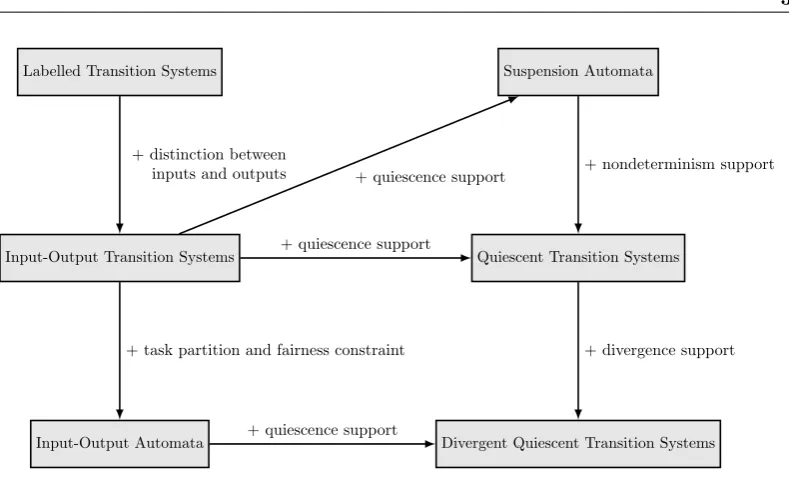
Figure 1.2: The various automata introduced in this thesis, and their main relationships.
Finally, we conclude our thesis by comparing the SA, QTS and DQTS models. Using (D)QTSs rather than SAs to model systems clearly offers several advantages. First of all, a wider range of systems can be modelled because the determinism and convergence require-ments of SAs have been dropped. Furthermore, the desirable compositional properties of (D)QTSs ensure that when using a testing framework likeioco, the specifications of com-plex systems can easily be divided up, modelled as separate components, and tested more efficiently. Hence, (D)QTSs look like a promising new formalism in the context of model-based testing.
Chapter
2
Background
In this chapter, we review three important system specification models from the literature: Labelled Transitions Systems (LTSs), which model systems using states, actions and tran-sitions; Input-Output Transition Systems (IOTSs), which extend LTSs by distinguishing between input and output actions; and finally Input-Output Automata, which further ex-tend IOTSs with multiple internal actions and action partitions to formalise the notion of fair executions. For each of these models, we will define the standard operations of determin-isation, parallel composition and action hiding. The IOTS and IOA models constitute the basis for the Quiescent Transition System (QTS) and Divergent Quiescent Transition System (DQTS) models that we will introduce in Chapter 3 and Chapter 4, respectively. We will also introduce Suspension Automata (SAs), which are an extension of IOTSs that support the notion of quiescence, i.e., the observation of an absence of outputs. At the end of this chapter, a short overview of the main properties of the different models will be given.
2.1
Notational Preliminaries
Before introducing the various models, we first need to establish some standard notations.
A sequence σ=a1a2 . . . an is a (possibly infinite) ordered list of elements from a setL. We define the length ofσ, denoted|σ|, asn. The empty sequence is denoted. We useL∗ to denote the set of all finite sequences overL, Lωto denote the set of all infinite sequences over L, andL∞ to denote the set of all sequences overL, i.e., L∞ =L∗ ∪ Lω. Given two sequences ρ∈L∗ and υ ∈L∞, we denote the concatenation of ρand υ as ρ ·υ or simply ρ υ. Note that·ρ=ρ·=ρ.
The projection of an element a ∈ L on L0 ⊆ L, denoted a
L0, equals a if a ∈ L0
and otherwise. The projection of a sequenceσ =a σ0 is defined inductively by σ L0 =
(a σ0) L0 = (aL0) · (σ0 L0). The projection of a set of sequences Z is defined as ZL0={σL0|σ∈Z}.
We use℘(L) to denote thepower set of the setL. A setP ⊂℘(L) such that ∅∈/ P is a
partition ofLifSP =L andp
6=qimpliesp∩q=∅for allp, q∈P.
Finally, we follow [BK08] in using the notation ∃∞ for ‘there exist infinitely many’.
Hence, the (valid) statement ‘there exist infinitely many integers greater than zero’ can be denoted as ∃∞j∈
Z. j >0.
s0
s1 s2
s3
s5
s4
s6
a a
τ
b
τ
c
(a)A
{s0}
{s1, s2, s3, s4}
{s5} {s6}
a
b c
(b)det(A)
s0
s1
s2
s4
s3
s5
a τ
τ
b τ
τ
c
[image:14.595.148.496.138.274.2](c)B
Figure 2.1: Visual representations of the LTSsA,det(A) andB.
2.2
Labelled Transition Systems
2.2.1
The LTS Model
Labelled Transition Systems (LTSs) are a well-known formalism for modelling the behaviour of processes or systems. A LTS consists of a set of states, a set of transitions between these states, and a set of actions. Each state of the LTS represents a particular state which the process or system may occupy during its operation. The set of transitions define how the LTS can move from one state to the other by executing particular actions from the set of actions. With every LTS a special label τ is associated, which represents an unobservable, internal action.
Definition 2.1. A Labelled Transition System (LTS) is a tuple A = hS, S0, L,→ i, such
that:
• S is a non-empty set of states;
• S0⊆S is a non-empty set of initial states;
• Lis a set of labels, each representing a different action. We requireτ /∈L;
• → ⊆S×(L ∪ {τ})×S is the transition relation, and defines the transitions that are possible between the states of the LTS. Each transition is marked with a label to indicate which action is responsible for the transition.
We defineLτ =L∪ {τ}.
Given a LTSA, we denote its components bySA,SA0,LAand→A; we omit the subscript
when it is clear from the context which LTS is referred to. We will use the terms label and action interchangeably.
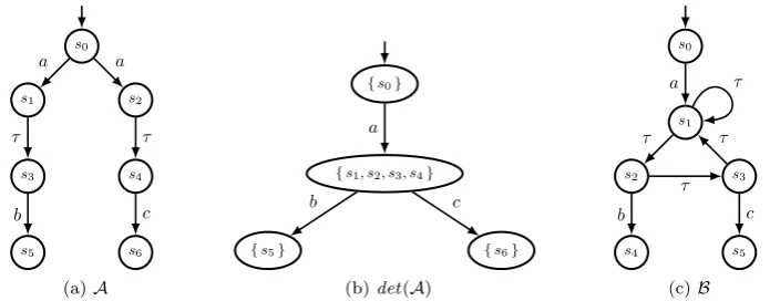
Example 2.2.Figure 2.1a visualises a LTSAwithSA={s0, s1, s2, s3, s4, s5, s6},SA0 ={s0},
andLA={a, b, c}. We represent states by circles and transitions by arrows; each arrow in
2.2. Labelled Transition Systems 7
Throughout this report, we use the following notations to describe transitions between states.
Definition 2.3 (Transitional notations). LetA=hS, S0, L,→ ibe an LTS withs, s0 ∈S,
a, ai ∈Lτ,b, bi∈L, and σ∈L∞, then
s−→a s0 =def (s, a, s0)∈ →
s−−−−−−a1·...·a→n s0 =
def ∃s0, . . . , sn∈S . s=s0−−a→ · · · −1 a−→n sn =s0 s−→a =def ∃s00∈S . s−→a s00
s 6−a
→ =def @s00∈S . s−→a s00
s=⇒ s0 =def s=s0 ors−τ−−−·...·→τ s0
s=⇒b s0 =def ∃s0, s1∈S . s=
⇒s0→−b s1=
⇒s0 s=b1·...·bn
====⇒s0 =
def ∃s0, . . . , sn∈S . s=s0=
b1
=⇒ · · ·=bn
=⇒sn=s0 s=σ⇒ =def ∃s00∈S . s=σ⇒s00
s=6σ⇒ =def @s00∈S . s=σ⇒s00
Ifs−→a for a s∈S anda∈Lτ, we say thataisenabled ins. We useL(s) to denote the set of all actionsa∈Lτ that are enabled in the states∈S, i.e.,L(s) ={a∈Lτ |s
−→ }a .
Example 2.4. Consider the LTSAin Figure 2.1a. The following statements all apply toA: s3−→b s5, s0−a τ b−−→s5, s4−→c , s3→6−c ,
s1=⇒ s3, s0=a b=⇒s5, s0=a c=⇒, s0=a b c==6 ⇒
Furthermore,L(s0) ={a}and L(s5) =∅.
We will use the following language notations to denote various aspects of LTSs and their behaviour.
Definition 2.5 (Language notations). LetA=hS, S0, L,→ ibe an LTS, then:
• A path in Ais an alternating sequence of states and actions that can be either finite or infinite. A finite path is a finite sequence π=s0a1s1a2s2 . . . sn such that for all 1 ≤ i ≤ n we have si−1 −−a→i si with si ∈ S, ai ∈ L. An infinite path is an infinite sequence π=s0a1s1a2s2. . . such that for alli≥1 we havesi−1−−a→i si withsi ∈S, ai∈L. A pathπ=s0a1s1a2s2 . . . is calledcyclic ifsi=sj for somei6=j.
• The set of all paths inAis denotedpaths(A). The path operator first yields the first state on a given path, e.g., for π=s0a1s1 we have first(π) =s0. The path operator
states yields the set of states that occur on a given pathπ, i.e.,states(π) =πS. For example, forπ=s0a1s1τ s0a2s2 we have states(π) ={s0, s1, s2}.
• For an infinite path π,ω-states(π) denotes the set of states that occur infinitely often on that path, i.e., for a pathπ=s0a1s1. . ., we define ω-states(π) ={s∈states(π)|
∃∞j . s
j =s}.
• The path operator trace yields the sequence of actions that is obtained by erasing all states and internal actions from a given path, i.e., trace(π) = π L. Such a sequence of actions is called a trace. For example, for π =s0a1s1τ s2a2s3 we have
trace(π) =a1a2.
• For every s∈S, traces(s) denotes the set of all traces of Athat correspond to paths that start in s, i.e., traces(s) = {trace(π) | π ∈ paths(A) ∧ first(π) = s}. The set of all traces that correspond to paths that start in one of the start states of Ais denotedtraces(A) =S
s∈S0traces(s). Two LTSsBandCaretrace equivalent, denoted
• For a finite traceσ and state s ∈ S, reach(s, σ) denotes the set of states in A that can be reached froms viaσ, i.e.,reach(s, σ) ={s0 ∈S |s=σ⇒s0}; for a set of states S0 ⊆S, reach(S0, σ) denotes the set of states that can be reached from a state inS0, i.e.,reach(S0, σ) =S
s∈S0reach(s, σ).
We add subscripts to these language notations to indicate the LTS they refer to, in case this is not clear from the context.
Example 2.6. First, consider again the LTSA in Figure 2.1a. Clearly, s0a s1τ s3b s5 and
s0a s2τ s4c s6 are finite paths of A. We have traces(A) ={, a, a b, a c}. Furthermore, we
find thatreach(s0, a) ={s1, s2, s3, s4}and reach({s1, s4}, ) ={s1, s3, s4}. Now, consider
the LTS B in Figure 2.1c. Both π1 =s0a s1τ s1τ s1 . . . and π2 =s1τ s2τ s3τ s1τ s2 . . .
are infinite paths of B. In this case, we have ω-states(π1) = {s1} and ω-states(π2) =
{s1, s2, s3}.
A fundamental concept in automata theory is the notion of determinism.
Definition 2.7 (Determinism). An LTSA isdeterministic if the following two conditions hold:
1. for alls, s0∈S anda∈Lτ, ifs
−→a s0 , thena6=τ;
2. for alls, s0, s00∈S anda∈L, ifs−→a s0 ands−→a s00, thens0=s00. Otherwise,Aisnondeterministic.
Example 2.8. The LTSA in Figure 2.1a is nondeterministic, since both of the transitions s0 −→a s1 and s0 −→a s2 are enabled in s0. Hence, if a is observed in state s0, we do not
know beforehand whether we end up in state s1 or s2. Furthermore, A contains several
τ-transitions.
When considering infinite paths, the notion of divergence (and convergence) is important. Definition 2.9 (Divergence). Let A be an LTS and letπ ∈ paths(A) be an infinite path in A. The path π isdivergent if it contains only internal transitions, i.e., ai =τ for every action ai on π. The set of divergent paths of A is denoted dpaths(A). If A contains any divergent paths, then it is called divergent; otherwise,Aisconvergent.
Example2.10. Consider the LTSBin Figure 2.1c. The infinite pathπ=s1τ s2τ s3τ s1τ s2. . .
of B is divergent, as it contains only internal transitions. Futhermore, since |states(π)| = |{s1, s2, s3}|= 3,πis bounded.
2.2.2
Operations
In this section, we take a look at some of the standard operations that can be applied to LTSs: determinisation, parallel composition and action hiding. It is a well-known fact from the literature that LTSs are closed under all three operations.
2.2. Labelled Transition Systems 9
a
τ
b
(a)A
a
τ
c
(b)B
a
τ τ
b τ τ c
τ
b c
τ
c b
[image:17.595.131.406.141.292.2](c)A k B
Figure 2.2: The LTSsAandB, and their parallel compositionA k B.
Definition 2.11 (Determinisation of LTSs). The determinisation of an LTS A = hS, S0, L,→
Aiis the LTSdet(A) =hSD, SD0, L,→Di, whereSD,SD0 and→Dare defined as
follows:
SD = ℘(S)\ ∅
S0
D = {S0}
→D = {(U, a, V)∈SD×L×SD | V =reachA(U, a) ∧ V 6=∅ }
Example 2.12. The determinisation of the nondeterministic LTSAin Figure 2.1a is shown in Figure 2.1b. In this case, the four individual statess1, s2, s3 ands4 ofA are condensed
into one single composite state indet(A), sincereach(s0, a) ={s1, s2, s3, s4}. Note also that
indeedA ≈tr det(A).
Next, we introduce the parallel composition operator. This operator is fundamental in modelling frameworks for component-based design. It allows one to build complex system models from smaller ones, thus breaking up the specification of a system into manageable pieces. Parallel composed LTSs synchronise on shared actions, and can execute the internal actionτ and non-shared actions indepedently from each other.
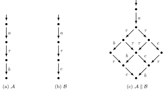
Definition 2.13 (Parallel composition of LTSs). Given two LTSs A=hSA, S0A, LA,→Ai
and B = hSB, SB0, LB,→Bi, the parallel composition of A and B is the LTS A k B =
hSAkB, SAkB0 , LAkB,→AkBi, where SAkB,SAkB0 , LAkBand→AkB are defined as follows:
SAkB = SA×SB
S0
AkB = SA0 ×SB0
LAkB = LA∪LB
→AkB = {((s, t), a,(s0, t0))∈SAkB×(LA∩LB)×SAkB | s−→a As0 ∧ t−→a Bt0}
∪ {((s, t), a,(s0, t))∈SAkB×((LA\LB)∪ {τ})×SAkB | s−→a As0}
∪ {((s, t), a,(s, t0))∈SAkB×((LB\LA)∪ {τ})×SAkB | t−→a Bt0}
The first clause of the definition of→AkB ensures that parallel composed LTSs
a
b τ
c
(a)A
τ
b τ
τ
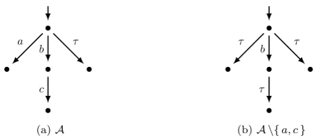
[image:18.595.206.435.136.236.2](b)A \{a, c}
Figure 2.3: The LTSsAandA \{a, c}.
Example 2.14. Figure 2.2 shows two LTSs Aand B, and their parallel compositionA k B. We have assumedLA={a, b, d}andLB={a, c, d}, henceLAkB={a, b, c, d}. Sinceaand
d are shared actions, the parallel composition A k B can only execute these actions when both component LTSs are able to, i.e.,A k Bsynchronises on theaanddactions. The other actions, including the internal action τ, can be executed independently.
Finally, it is often useful to hide certain actions of a LTS, thereby treating them as internal actions. For example, when parallel composing two LTSs, some actions are only used for synchronisation; after parallel composition, they are not needed anymore.
Definition 2.15 (Action hiding in LTSs). LetA=hS, S0, L,→Aibe an LTS andH ⊆LO
a set of output labels, then one canhideHinAto obtain the LTSA \H=hS, S0, LH,→Hi, whereLH and→H are defined as follows:
LH = L\H
→H = {(s, a, s0)∈ →A | a /∈H}
∪ {(s, τ, s0)∈S× {τ} ×S | ∃a∈H .(s, a, s0)∈ →A}
Hence, the hidden actions are removed from the set of actions, and all transitions for those actions become τ-transitions.
Example 2.16. Consider the LTSAin Figure 2.3a and assumeLA={a, b, c}. After hiding
the actionsaandc, the resulting IOTS isA \{a, c}, which is shown in Figure 2.3b. We have LA \{a,c}={b}.
2.3
Input-Output Transition Systems
2.3. Input-Output Transition Systems 11
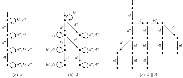
b?, c?
a?
a?, c?
b?
a?, b?, c?
d!
a?, b?, c?
(a)A
b?
a! d?
d?
b? c!
b?, d?
b?, d?
e!
b?, d?
b?, d?
a!
b?, d?
(b)A
a!
b?
c!
e!
d!
a!
b?
d!
b!
e! d!
d!
a!
d! a!
[image:19.595.87.451.140.296.2](c)A k B
Figure 2.4: The IOTSs Aand B, and their parallel composition A k B. Note that we have left out some of theb-labelled self-loops from the visualisation of A k Bto reduce clutter.
2.3.1
The IOTS Model
Definition 2.17 (Input-Output Transition Systems). An Input-Output Transition System
(IOTS) is a tupleA=hS, S0, LI, LO,→ i, such that: • S is a non-empty set of states;
• S0⊆S is a non-empty set of initial states;
• LI andLO are disjoint sets of input and output labels, respectively;
• → ⊆S×(LI∪LO∪ {τ})×S is the transition relation.
We defineL=LI∪LO andLτ=L∪ {τ}, and requireτ /∈L.
Remark 2.18. We often suffix a question mark (?) to input labels and an exclamation mark (!) to output labels, to help distinguishing the two types. These are, however, not part of the label.
The notations introduced in Definition 2.3 and Definition 2.5 for LTSs also apply to IOTSs. Compared to regular LTSs, IOTSs partition the set of labels into disjoint sets of input labels and output labels. Furthermore, we require every IOTS to beinput-enabled. Definition 2.19 (Input-enabledness). An IOTSA=hS, S0, LI, LO,→ iisinput-enabled if
s−→a for alls∈S and everya∈LI, i.e., Acan accept any input in any state.
Example 2.20. Figure 2.4a shows an IOTSAwithLI
A={a, b, c}andLOA={d}. Note that
Ais indeed input-enabled.
From now on, we assume that all given IOTSs are input-enabled, unless explicitly stated otherwise.
2.3.2
Operations
Similar to LTSs, IOTSs support the operations of determinisation, parallel composition and action hiding. Determinisation for IOTSs is exactly the same as for LTSs. Parallel compo-sition of IOTSs is different, since rather than synchronising on all shared actions like LTSs, parallel composed IOTSs synchronise on shared inputs and complementary input-output pairs, and cannot have shared outputs [DNS95]. Furthermore, when two inputs synchronise the result is an input transition in the composite automaton, and when a complementary input and output synchronise, the result is an output transition.
Definition 2.21(Parallel composition of IOTSs). Given IOTSsA=hSA, SA0, LIA, LOA,→Ai
and B=hSB, SB0, LIB, LOB,→Bisuch thatLOA∩LOB =∅, theparallel composition of Aand
B is the IOTSA k B =hSAkB, SAkB0 , LIAkB, LOAkB,→AkBi, whereSAkB, SAkB0 ,LIAkB, LOAkB
and→AkB are defined as follows:
SAkB = SA×SB
S0AkB = S0A×SB0
LIAkB = (LIA∪LBI)\(LOA∪LOB) LOAkB = LOA∪LOB
→AkB = {((s, t), a,(s0, t0))∈SAkB×(LA∩LB)×SAkB | s−→a As0 ∧ t−
a →Bt0} ∪ {((s, t), a,(s0, t))∈SAkB×((LA\LB)∪ {τ})×SAkB | s−→a As0}
∪ {((s, t), a,(s, t0))∈SAkB×((LB\LA)∪ {τ})×SAkB | t−→a Bt0}
We haveLAkB=LIAkB∪L
O
AkB=LA∪LB.
Example 2.22. Figure 2.4 shows two IOTSsAandB, and their parallel compositionA k B. We have assumed that LIA={a, b, c},LOA ={d}, LIB ={b, d}, andLOB ={a, c, e}. Note that indeedLOA∩LOB =∅, as required; henceLAkBI ={b}andLOAkB={a, c, d, e}.
Action hiding is exactly the same for IOTSs as for LTSs, except that only output actions can be hidden.
Definition 2.23 (Action hiding in IOTSs). LetA=hS, S0, LI, LO,→
Aibe an IOTS and
H ⊆ LO a set of output labels, then one can hide H in A to obtain the IOTS A \H =
hS, S0, LI, LO
H,→Hi, where LOH and→H are defined as follows: LO
H = LO\H
→H = {(s, a, s0)∈ →A | a /∈H}
∪ {(s, τ, s0)∈S× {τ} ×S | ∃a∈H .(s, a, s0)∈ →A}
Like LTSs, IOTSs are closed under the operations of determinisation, parallel composi-tion, and action hiding.
2.4
Input-Output Automata
2.4. Input-Output Automata 13
2.4.1
The IOA Model
Definition 2.24 (Input-Output Automata). AnInput-Output Automaton (IOA) is a tuple A=hS, S0, LI, LO, LH, P,→ i, such that:
• S is a non-empty set of states;
• S0⊆S is a non-empty set of initial states;
• LI,LO and LHare pairwise disjoint sets of input, output, and internal labels,
respec-tively;
• P is a partition of LO ∪ LH, i.e., a partition of the locally controlled actions, and is called the task partition;
• → ⊆S×(LI∪LO∪LH)×S is the transition relation.
We defineL=LI∪LO∪LH.
The intuition behind the task partition P is that each element of P represents the set of locally controlled actions under the control of a particular subcomponent of the whole system. Hence, an element of P may contain both outputs and internal transitions. The task partitionP plays an important role when it comes to the notion of fairness, as will be shown later on.
Similar to IOTSs, we require every IOA to be input-enabled. Clearly, for every IOTS A=hS, S0, LI, LO,→ i there exists a trace-equivalent IOA A0 =hS, S0, LI, LO, LH, P,→ i,
withLH={τ} andP ={LO∪ {τ} }.
Example 2.25. Let A be an IOA with LO
A = {a, b} and LHA = {c, d}. An example of a
partition of the locally controlled actions ofAwould bePA={ {a, c},{b, d} }. In this case,
Ais assumed to consist of two independent subcomponents, which control the sets of actions {a, c} and{b, d}, respectively.
Remark 2.26. IOAs are visualised in the same manner as IOTSs, with a question mark (?) for an input, and an exclamation mark (!) for an output. A label without a suffix is assumed to be an internal label.
The notations introduced in Definition 2.3 and Definition 2.5 for LTSs also apply to IOAs. However, since IOAs can have multiple internal labels, the transitional notation =⇒ is more general for IOAs than for LTSs and IOTSs, which only have one internal label (τ).
Definition 2.27 (Transitional notations for IOAs). LetAbe an IOA withs, s0 ∈S, then: s=⇒ s0 =def s=s0 or ∃a1, . . . , an∈LHA. s−−−−−−a1·...·a→n s0
The other transitional notations use this more general definition of =⇒ where applicable. Similarly, the definitions of determinism and divergence are more general for IOAs than for LTSs and IOTSs.
Definition 2.28 (Determinism in IOAs). An IOA A is deterministic if the following two conditions hold:
1. for alls, s0∈S anda∈L, ifs−→a s0 , thena /∈LHA;
s0
s1
s2
s4
s3
s5
a? b
b
e!
c d
f!
(a)A
s0
s2
s1 b
c!
a?
[image:22.595.206.439.137.275.2](b)B
Figure 2.5: The IOAs AandB. Note that suffixless labels indicate internal actions
Example 2.29. The IOAAin Figure 2.5a is nondeterministic, as it contains multiple transi-tions labelled with internal actransi-tions.
Definition 2.30 (Divergent path in IOAs). LetAbe an IOA andπ∈paths(A) an infinite path in A. The path π is divergent if it contains only transitions labelled with internal actions, i.e.,ai∈LHAfor every actionai onπ.
Example 2.31. Consider the IOAAin Figure 2.5a withLH
A={b, c, d}. Clearly, the infinite
pathss1b s1b s1 . . . ands1b s2c s3d s1b s2. . . are both divergent.
The notion of fairness plays an important role in IOAs (and Divergent Quiescent Tran-sition Systems, as will be explained in Chapter 4). The following definition of a fair path improves the notion of fair executions given in [LT87, LT89, DNS95], assuming that if an action from an element of P is infinitely often enabled in an infinite path, then an action from that same element of P must be executed infinitely often in that path.
Definition 2.32 (Fair path). Let A = hS, S0, LI, LO, LH, P,→ i be an IOA and π =
s0a1s1a2s2. . . a path of A. If π is an infinite path, then π is fair if, for every A ∈ P
such that ∃∞j . L(sj) ∩A 6= ∅, we have ∃∞j . a
j ∈A. Thus, if actions from A are in-finitely often enabled in the states of pathπ, then actions fromAare infinitely often executed in the pathπ. Ifπ is a finite path, thenπis fair by default. The set of all fair paths of an IOAAis denotedfpaths(A).
Hence, under this notion of fairness, each subcomponent of the system (represented by an element of the setP) that is infinitely often given the chance to execute some of its actions, will infinitely often execute some of its actions.
Example 2.33. Consider the IOABin Figure 2.5b. Clearly,π=s0b s0b s0 . . . is an infinite
path ofA. Now assume thatPA={ {b},{c} }; i.e., the internalb-action and thec-output
are controlled by two independent subcomponents. In this case, the pathπwould not be fair: the c-output, which belongs to a different partition than the internal b-action, is infinitely often enabled, but is never executed. The path π is only fair ifPA ={ {b, c} }. Hence, if
PA={ {b},{c} }, then fpaths(A) =∅, but ifPA={ {b, c} }, thenfpaths(A) ={π}.
2.4. Input-Output Automata 15
2.4.2
Operations
The determinisation of IOAs proceeds exactly the same as for LTSs and IOTSs. The op-eration of parallel compositon is also applicable to IOAs. However, since IOAs can have multiple internal actions and also have an associated partition of the locally controlled ac-tions, we need to impose some additional constraints to ensure that the component IOAs in a parallel composition do not use internal actions to communicate, and that every locally controlled action of the parallel composition is under the control of at most one component IOA [LT87, LT89]. Two IOAs that satisfy these constraints are said to be compatible.
Definition 2.34 (IOA compatibility). Two IOAsA=hSA, SA0, LAI , LOA, LHA, PA,→Aiand
B=hSB, S0B, LIB, LBO, LHB, PB,→Biare compatible if their sets of ouput actions are disjoint,
and no internal action of either appears as an input, output or internal action of the other, i.e.,AandBare compatible ifLOA∩LOB =∅,LHA∩LB=∅, andLHB ∩LA=∅.
Two compatible IOAs can be parallel composed in a similar way as IOTSs, as the next definition shows.
Definition 2.35 (Parallel composition of IOAs). LetA =hSA, S0A, LIA, LOA, LHA, PA,→Ai
and B =hSB, SB0, LIB, LOB, LHB, PB,→Bi be two compatible IOAs. The parallel composition
ofAandBis the IOAA k B=hSAkB, SAkB0 , L
I
AkB, L
O
AkB, L
H
AkB, PAkB,→AkBi, whereSAkB,
S0
AkB,L
I
AkB,L
O
AkB,L
H
AkB, PAkB and→AkB are defined as follows:
SAkB = SA×SB
S0
AkB = SA0 ×SB0
LI
AkB = (LIA∪LIB)\(LOA∪LOB)
LO
AkB = LOA∪LOB
LH
AkB = LHA∪LHB
PAkB = PA∪PB
→AkB = {((s, t), a,(s0, t0))∈SAkB×(LA∩LB)×SAkB | s−→a As0 ∧ t−→a Bt0}
∪ {((s, t), a,(s0, t))∈SAkB×(LA\LB)×SAkB | s−→a As0}
∪ {((s, t), a,(s, t0))∈SAkB×(LB\LA)×SAkB | t−→a Bt0}
We have LAkB=LIAkB∪LOAkB∪LHAkB=LA∪LB.
Hence, the partition of locally controlled actions for the parallel composition is simply the union of the partitions of the locally controlled actions of the component IOAs. The constraints imposed by the compatibility requirement ensure that this is indeed a valid partition.
The hiding of actions in an IOA is rather straightforward.
Definition 2.36(Action hiding in IOAs). Given an IOAA=hS, S0, LI, LO, LH, P,→ iand
a set of outputsH ⊆LO,hidingH in Ayields the IOAA \H =hS, S0, LI, LO
H, LHH, P,→ i, whereLO
H =LO\H and LHH=LH∪H.
Thus, the hiding operation simply removes the output labels that are to be hidden from the set of outputs, and adds them to the set of internal labels.
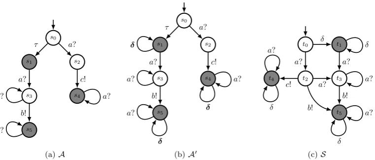
s0
s1 s2
s3
s5
s4
τ a?
a? a? b! c! a? a? (a)A s0 s1 s2 s3 s5 s4
τ a?
δ a? a? b! c! a? a? δ δ
(b)A0
[image:24.595.134.515.138.300.2]t0 t1 t2 t3 t4 t5 δ a? δ a? a? b! c! b! a? a? δ a? δ (c)S
Figure 2.6: Visual representation of the construction of the SA S that corresponds to the IOTSA, alongside the intermediate automatonA0.
2.5
Suspension Automata
As discussed in Section 2.3, Input-Output Transition Systems (IOTSs) can be used to model the reactive behaviour of a system in terms of inputs and outputs, but cannot explicitly express the observation of the absence of outputs, also called quiescence [Vaa91, Seg97]. For this, the so-called Suspension Automata (SAs) [Tre96a, Tre96b], an extension of regular IOTSs, are used. These automata can be used to model all possible observations for a par-ticular system, including quiescence, and can thus be thought of as ‘observation automata’. In this section, we give a short overview of SAs.
First of all, a concept that plays an important role in SAs is the so-calledquiescent state. A quiescent state from which the system cannot proceed autonomously, without inputs from the environment; i.e., a quiescent state is a state in which no output or internal transitions can be exceuted [Tre96a, Tre96b].
Definition 2.37 (Quiescent state). Let A be an IOTS. A state s ∈ S is quiescent if no outputs or internal transitions are enabled in that state, i.e., sis called quiescent if for all a∈LO∪ {τ} we haves
6−a →.
Example 2.38. Consider the IOTS A in Figure 2.6a. The states marked in gray are all quiescent, as these states have no outgoing output or internal transitions.
Rather than being built from scratch like regular IOTSs, a SA is constructed by taking an existing (convergent) IOTS and adding δ-labelled self-loops to its quiescent states, and determinising the result [Tre08]. Theδ-label is a special kind of output label that represents the observation of quiescence, and is not part of the actual output setLO.
Definition 2.39(Suspension Automata). Given an IOTSA=hS, S0
A, LI, LO,→ i, letA0 =
hS, S0
A, LI, LO,→0iwhere→0 = → ∪ {(s, δ, s)∈S× {δ} ×S|sis quiescent in A }. The
Suspension Automaton corresponding to Ais then the IOTSS =det(A).
Example 2.40. Figure 2.6 visualises how a SA is constructed for the IOTS A shown in Figure 2.6a. First, the automatonA0 is obtained fromAby introducing newδ-labelled
self-loops (marked in bold) for the quiescent states of A. Next,A0 is determinised, resulting in
2.6. Summary 17
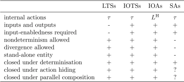
Table 2.1: Comparison of the features of LTSs, IOTSs, IOAs and SAs.
LTSs IOTSs IOAs SAs
internal actions τ τ LH τ
inputs and outputs - + + +
input-enabledness required - + + +
nondeterminism allowed + + +
-divergence allowed + + +
-stand-alone entity + + +
-closed under determinisation + + + +
closed under action hiding + + + ?
closed under parallel composition + + + ?
Since a SA captures all possible observations of a given IOTS, including quiescence, SAs are perfectly suited to model the behaviour of both specifications and implementations in model-based testing frameworks such as the industry-leading ioco [Tre96a, Tre96b] frame-work. The ioco framework, in turn, is used by well-known test generation tools likeTGV [JT05], theAgedis Tool Set[HN04],TestGen[HT99], andTorX[BFd+99, TB03].
However, SAs have some major limitations [Tre08]. First of all, SAs can only be con-structed for convergent IOTSs, since it is not clear how the notions of divergence and quies-cence can be reconciled. Furthermore, SAs must necessarily be deterministic. Both of these requirements clearly limit the number of systems that can be effectively modelled as SAs. SAs are also implicitly defined: they can only be constructed by taking an existing IOTS and applying the transformations described in Definition 2.39; they cannot be built from scratch. Finally, the closure properties of SAs regarding parallel composition and action hiding have not been investigated, and are therefore unknown. Hence, there is no fully formalised theory for SAs. In the next chapter, we introduce Quiescent Transition Systems (QTSs), which also extend IOTSs with the notion of quiescence, and address all these shortcomings of SAs, except the convergence requirement. This requirement will in turn be lifted by Divergent Quiescent Transition Systems (DQTSs), which will be introduced in Chapter 4.
2.6
Summary
In this chapter, we have introduced Labelled Transition Systems (LTSs), Input-Output Tran-sition Systems (IOTSs) and Input-Output Automata (IOAs). LTSs are used to model the behaviour of systems using states, transitions, a set of actions, and a special internal ac-tion τ. IOTSs extend LTSs by distinguishing between input actions and output actions. IOAs further generalise IOTSs by allowing multiple internal actions and partitioning the set of locally controlled actions (output actions and internal actions) to formalise the notion of fair executions.
Chapter
3
Quiescent Transition Systems
This chapter introduces Quiescent Transition Systems (QTSs). Like the Suspension Au-tomata (SAs) described in Section 2.5, QTSs are a specialisation of regular IOTSs that sup-port the notion of quiescence. However, a QTS need not necessarily be deterministic, and can be built from scratch, whereas SAs are implicitly defined and have to be deterministic.
Furthermore, in this chapter we also closely examine several closure and commutativity properties of QTSs with regards to the determinisation, parallel composition and action hiding operations, something which has not been done for SAs. Finally, we also define what exactly it means for a QTS to be well-formed, thus establishing the semantic validity of the model. Note that the convergence requirement of SAs also applies to QTSs. This requirement will be lifted by the Divergent Quiescent Transition Systems (DQTSs) introduced in the next chapter.
Remark 3.1. A basic variant of QTSs was already used in [TBS11] in a testing framework. An earlier version of the QTS model described here has been published previously by the author in [STS12a, STS12b].
3.1
The QTS Model
As mentioned earlier, QTSs, like SAs, are a specialisation of regular IOTSs in which the observation of quiescence is explicitly modelled with a specialδ-label.
Definition 3.2 (Quiescent Transition Systems). A Quiescent Transition System (QTS) is a tupleA=hS, S0, LI, LO,→ i, where:
• S is a non-empty set of states;
• S0⊆S is a non-empty set of initial states;
• LI and LO are disjoint sets of input and output labels, respectively. As for regular
IOTSs, we require τ /∈LI ∪LO. Furthermore, δ /∈LI ∪LO is a special output label
that is used to denote the observation of quiescence; • → ⊆S×(LI∪LO∪ {τ, δ})×S is the transition relation.
As for IOTSs, we defineL=LI ∪LO and Lτ =L ∪ {τ}. Given a QTSA, we denote its components bySA, SA0, LIA, LOA and →A; we omit the subscript when it is clear from the
context which QTS is referred to.
s0
s1 s2
s3
s5
s4
s6
τ τ
a?, c?
c?, δ a?
a?, c?
b!
a?, δ c?
a?, c?
d!
a?, c? a?, c?
[image:28.595.252.392.129.284.2]δ δ
Figure 3.1: Visual representation of a QTSA. The gray states are quiescent.
Like regular IOTSs, QTSs must be input-enabled. All other definitions introduced in Section 2.3 for IOTSs also apply to QTSs. As an important restriction, we do not allow divergent paths to occur in (regular) QTSs. As said earlier, this restriction will be lifted in DQTSs, which will be introduced in Chapter 4. Note that, similar to theδ-label of SAs, the δ-label is a special output label and is not part of LO, the set of regular outputs.
Example3.3.Figure 3.1 visualises a nondeterministic QTSA. Note theδ-labelled transitions, which represent the observations of quiescence, i.e., the absence of enabled outputs.
As mentioned in Definition 2.37, we distuinguish a special kind of state in IOTSs: the so-called quiescent state. For convenience’ sake, we repeat the definition here and apply it to QTSs, and also introduce a notation for such states. Recall that a δ-labelled transition originating from such a state represents the absence of locally controlled behaviour, i.e., the observation of quiescence.
Definition 3.4 (Quiescent states of IOTSs or QTSs). LetAbe an IOTS or QTS. A state s ∈ S is quiescent, denoted q(s), if no locally controlled actions are enabled in that state, i.e.,q(s) if for alla∈LO∪ {τ}we haves 6−a
→. The set of all quiescent states ofAis denoted
q(A).
Example 3.5. Consider again the QTSAin Figure 3.1. Statess1,s2,s5ands6are quiescent,
since no locally controlled actions (in this case, the internal actionτ and the outputsband d) are enabled in those states. Note that state s0 is not quiescent, as the internal action is
enabled in this state.
A system in a quiescent state will be idle until a new input is supplied, and hence quies-cence may be observed in such a state.
An important detail to note: we consider a states in which aτ-transition is enabled to not be quiescent, even if there is no regular output a ∈ LO that is enabled in s. In this,
3.2. Well-formedness 21
δ a?
δ
a?
b!
c!
a?, δ
a?, δ a?
a?
(a)A
δ
a?
δ
a?
a?
b!
c! d! d! b!
a?
a?, δ a?, δ a?, δ
a?
b!
a?
a?, δ a?, δ
δ
[image:29.595.117.426.140.280.2](b)B
Figure 3.2: The QTSs AandBthat do not satisfy rule R3 and R4, respectively.
3.2
Well-formedness
In the previous sections, we have introduced QTSs, quiescent states andδ-transitions, but have not yet imposed any restrictions regarding the occurrence ofδ-transitions. For instance, it is possible for a QTS to have a δ-transition that leads to a state in which outputs are enabled, but that would contradict the semantics of theδ-transition. As a consequence, the observable behaviour of a syntactically correct QTS might not correspond to any realistic specification or implementation. To exclude such situations, we define four additional rules that define exactly which QTSs exhibit correct behaviour. Such QTSs are calledwell-formed. Definition 3.6 (Well-formedness for QTSs). A QTSA=hS, S0, LI, LO,→ iiswell-formed
if it satisfies the following four rules for all statess, s0, s00∈S and inputsa∈LI:
Rule R1(Quiescence should be observable): ifq(s), thens−→δ .
This rule requires that each quiescent state has an outgoingδ-transition, since in these states quiescence may be observed, as discussed earlier.
Rule R2(Quiescent state after observation of quiescence): ifs−→δ s0, thenq(s0).
This rule demands that a quiescent state is entered after a δ-transition, i.e., no output or internal transition may take place before a new input is provided. Note that a δ -transition may still take place. Since the notion of timing plays no role of QTSs, there is no particular observation duration associated with quiescence. Hence, a δ-transition means that the system has not produced any outputs indefinitely; therefore, enabling any outputs after aδ-transition would clearly be erroneous. Internal transitions are also not allowed directly after aδ-transition, as this simplifies the theory and ensures consistency with Definition 3.4. Again, since internal actions are not observable, this restriction does not affect the possible external (observable) behaviour of the system.
Rule R3(Quiescence introduces no new behaviour): ifs−→δ s0, thentraces(s0)⊆traces(s).
This is counterintuitive, since there is no notion of timing associated with the QTS model. Hence, behaviour is enabled either immediately or not at all, but quiescence should never enable new behaviour.
Rule R4 (Continued quiescence preserves behaviour): if s −→δ s0 and s0 −→δ s00, then
traces(s00) =traces(s0).
This rule ensures that the behaviour that can be observed after a single observation of quiescence, is the same as the behaviour that can be observed after multiple observations of quiescence in a row. This rule prohibits a situation as in the QTSB in Figure 3.2b. Here, the behaviour after two δ-transitions differs from the behaviour after the first. Since quiescence represents the fact that no outputs are observed and there is no notion of timing in the QTS model, there can be no difference between observing it once or multiple times in succession.
From now on, we assume that all given QTSs are well-formed.
Note that a trace of a QTS can contain a sequence of δ-actions. Although this might seem odd, it corresponds to the practical testing scenario of observing a time-out rather than an output more than once in a row.
In Section 3.6, we fully discuss the rationale behind these well-formedness rules and look at some alternative rules.
Remark 3.7. In [Wil07] a definition forvalid deterministic SAs is given, alongside four condi-tions to which valid SAs should conform. These rules, although denoted differently, coincide exactly with the (less complex) rules R1, R2, R3 and R4 given above. Hence, valid SAs and well-formed QTSs form the same subclass of quiescence-enabled IOTSs.
3.3
Deltafication: from IOTS to QTS
Usually, the specification and implementation of a system are given as IOTSs, rather than QTSs. During testing, however, we typically observe the outputs of the system generated in response to inputs from the environment; thus, it is useful to be able to refer to the absence of outputs (i.e., quiescence) explicitly. Hence, we need a way to convert an IOTS to a QTS that captures all possible observations of it, including quiescence; this conversion is called deltafication and similar to the way SAs are constructed from IOTSs.
Definition 3.8 (Deltafication of IOTSs). Let A = hS, S0, LI, LO,→
Ai be an IOTS with
δ /∈L. The deltafication of Ais the QTS δ(A) =hS, S0, LI, LO,→
δi, where →δ is defined as follows:
→δ = →A ∪ {(s, δ, s)∈S× {δ} ×S|s∈q(A)}
Thus, the deltafication of an IOTSA simply adds δ-labelled self-loops to all quiescent states inA.
Example 3.9. Consider the IOTS Ain Figure 3.3a. The quiescent states ofAares1,s3, s5
and s6, and have been marked gray. As a result, these states acquire aδ-labelled self-loop
in the deltafication ofA, i.e.,δ(A), as shown in Figure 3.3b.
3.3. Deltafication: from IOTS to QTS 23
s0
s1 s2
s3 s4
s5 s6
b! a?
a?
a?
τ
τ
a? a?
a? a?
(a)A
s0
s1 s2
s3 s4
s5 s6
b!
a?, δ
a?
τ a?
τ δ
a? a?
a?, δ a?, δ
[image:31.595.97.441.137.274.2](b)δ(A)
Figure 3.3: Deltafication of an IOTSA.
Proof. Let A = hS, S0, LI, LO,→Ai be an IOTS such that δ /∈ L, and let δ(A) =
hS, S0, LI, LO,→δi be its deltafication, as defined in Definition 3.8. To show that δ(A) is a well-formed QTS, we need to prove thatδ(A) satisfies each of the rules R1, R2, R3 and R4. In the following, we usetracesδ(s) to denote the set of all traces ofδ(A) starting in the states∈S.
1. To prove thatδ(A) satisfies rule R1, we must show that for all statess∈S:
ifq(s), thens−→δ δ
Let s ∈ S be any state such that q(s) holds in δ(A). Since deltafication doesn’t change any existing transitions,q(s) then also holds in A. By Definition 3.8, we have (s, δ, s)∈ →δ after deltafication and therefores−→δ δ.
2. To prove thatδ(A) satisfies rule R2, we must show that for all statess, s0∈S:
ifs−→δ δ s
0, then q(s0)
Consider any transition s −→δ δ s
0 in δ(A) with s, s0 ∈ S. By Definition 3.8, we have
s=s0, and s(and therefore alsos0) is quiescent.
3. To prove thatδ(A) satisfies rule R3, we must show that for all statess, s0∈S:
ifs−→δ δ s
0, thentraces
δ(s0)⊆tracesδ(s)
Consider any transition s −→δ δ s
0 in δ(A) with s, s0 ∈ S. By Definition 3.8, we have
s=s0, and thereforetracesδ(s0)⊆tracesδ(s).
4. To prove thatδ(A) satisfies rule R4, we must show that for all statess, s0, s00∈S:
ifs−→δ δ s
0 ands0
−δ →δ s
00, thentraces
δ(s00) =tracesδ(s0)
Consider any pair of transitions s−→δ δ s
0 and s0
−δ →δ s
00 with s, s0, s00 ∈ S. By
δ
a? b?
a?, b?
c!
a?, b?
d!
δ a?, b?
δ
a?, b?
(a)A
a!
b!
δ
(b)B
a!
b! c!
c!
δ
b!
δ
[image:32.595.169.475.133.288.2](c)A k B
Figure 3.4: The QTSsA, B, and their parallel compositionA k B.
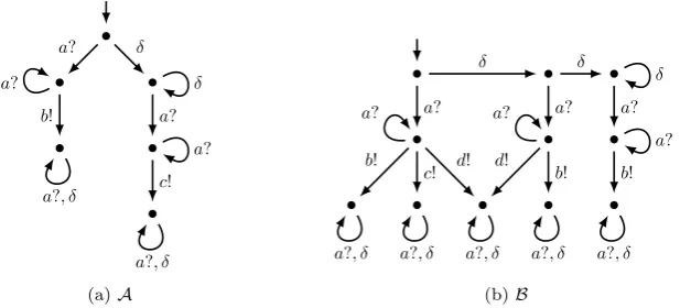
3.4
Operations
Since QTSs are a specialisation of IOTSs, all operations that are applicable to IOTSs (such as determinisation, parallel composition and hiding of actions) are also applicable to QTSs. Determinisation for QTSs is exactly the same as for IOTSs, but there are some minor differ-ences for parallel composition and action hiding.
3.4.1
Parallel Composition
Similar to IOTSs, we require parallel composed QTSs to synchronise on shared inputs and complementary input-output pairs. However, we also require QTSs to synchronise on δ -transitions, as a parallel composition of two QTSs can only be quiescent when both compo-nent QTSs are.
Definition 3.11 (Parallel composition of QTSs). LetA=hSA, S0A, LIA, LOA,→AiandB=
hSB, SB0, LIB, LOB,→Bi be two QTSs such thatLOA ∩ LOB = ∅. The parallel composition of
A andB is the QTSA k B=hSAkB, S0AkB, LIAkB, LOAkB,→AkBi, whereSAkB,SAkB0 , LIAkB,
LOAkB and→AkB are defined as follows:
SAkB = SA×SB
SAkB0 = SA0 ×SB0
LIAkB = (LIA∪LBI)\(LOA∪LOB) LOAkB = LOA∪LOB
→AkB = {((s, t), a,(s0, t0))∈SAkB×((LA∩LB)∪ {δ})×SAkB | s−→a As0 ∧ t−
a →Bt0} ∪ {((s, t), a,(s0, t))∈SAkB×((LA\LB)∪ {τ})×SAkB | s−→a As0}
∪ {((s, t), a,(s, t0))∈SAkB×((LB\LA)∪ {τ})×SAkB | t−→a Bt0}
As with parallel composed IOTSs, we have LAkB=LIAkB∪L
O
AkB=LA∪LB.
The first clause of→AkBensures that parallel composed QTSs synchronise both on shared
3.5. Properties 25
s0 s1
s2
a!
τ b!
(a)A
s0 s1
s2
τ
τ b!
(b)A \{a}
Figure 3.5: The QTSsAandA \{a}.
Example 3.12. See Figure 3.4 for two QTSs AandB, and their parallel compositionA k B. Note the synchronisation on theδ-transitions.
3.4.2
Action Hiding
The hiding of outputs in QTSs is exactly the same as for IOTSs, except that we do not allow the special output labelδ to be hidden, as this label doesn’t represent a specific output but rather (the observation of) a lack of outputs. Furthermore, since we disallow divergent paths in QTSs, we do not allow the hiding of output labels to lead to the creation ofτ-loops, i.e., cyclic divergent paths.
Definition 3.13 (Action hiding in QTSs). Let A = hS, S0, LI, LO,→
Ai be a QTS and
H ⊆ LO a set of output labels. If A does not contain a cyclic path s
0a1s1a2 . . . such
that for all ai we have ai ∈ H ∪ {τ}, then one can hide H in A to obtain the QTS A \H =hS, S0, LI, LO
H,→Hi, whereLOH and→H are defined as follows: LOH = LO\H
→H = {(s, a, s0)∈ →A | a /∈H}
∪ {(s, τ, s0)∈S× {τ} ×S | ∃a∈H .(s, a, s0)∈ → A}
Example 3.14. Consider the QTS Ain Figure 3.5a and assume LA={a, b}. After hiding
the output actiona, the resulting QTS is A \{a}, which is shown in Figure 3.5b. We have LA \{a} ={b}. Note that we cannot hide both the output actions a andb, as this would
result in theτ-loops0τ s1τ s2τ s0.
3.5
Properties
In this section, we present several important results regarding QTSs. First, they are closed under all operations mentioned previously. Second, they have many useful commutativity properties regarding function composition of deltafication and the other operations.
3.5.1
Closure Properties
It turns out that well-formed QTSs are closed under all operations defined thus far: deter-minisation, parallel composition, and action hiding. Therefore, these operations are indeed well-defined for well-formed QTSs.
Proof. Let A = hS, S0, LI, LO,→
Ai be a well-formed QTS and let det(A) =
hSD, SD0, L
I, LO,→
Di be its determinisation, as defined in Definition 2.11. To prove that
well-formed QTSs are closed under determinisation we must show that det(A) is a well-formed QTS, i.e., that it satisfies each of the rules R1, R2, R3 and R4. In the following, we usetracesD(U) to denote the set of all traces ofdet(A) starting in the stateU ∈SD.
1. To prove thatdet(A) satisfies rule R1, we must show that for all statesU ∈SD:
ifq(U), thenU −→δ D
LetU ∈SD be any state such that q(U) holds in det(A). This implies that all states
s ∈ U are quiescent in A. From rule R1 it follows that for every state s ∈ U there exists another state s0 ∈ S such that s −→δ A s0. Therefore reachA(U, δ) 6= ∅. By
Definition 2.11, we then have (U, δ,reachA(U, δ))∈ →D. Thus,U→−δ D.
2. To prove thatdet(A) satisfies rule R2, we must show that for all statesU, V ∈SD:
ifU −→δ DV, thenq(V)
Consider any transitionU −→δ DV withU, V ∈SD. IfU −→δ DV, then, by Definition 2.11,
V =reachA(U, δ) andV 6=∅. Hence, for every states0 ∈V there exists a state s∈U
such thats−→δ As0. Using rule R2 we can then conclude that everys0 ∈V is quiescent
inA, thusq(V) holds indet(A).
3. To prove thatdet(A) satisfies rule R3, we must show that for all statesU, V ∈SD:
ifU −→δ DV, thentracesD(V)⊆tracesD(U)
Consider any transition U −→δ D V with U, V ∈ SD. Assume σ ∈ tracesD(V). We
must show that alsoσ∈tracesD(U). If σ∈tracesD(V), then there clearly must exist
a state s0 ∈ V such that s0 =σ⇒A. Since U −→δ D V, it follows from Definition 2.11
that V = reachA(U, δ) andV 6=∅. Hence, there must exist a state s∈ U such that
s −→δ A s0. Using rule R3 we can then conclude that tracesA(s0) ⊆ tracesA(s), and
therefores=σ⇒A. Sinces∈U, it follows thatσ∈tracesD(U).
4. To prove thatdet(A) satisfies rule R4, we must show that for all statesU, V, W ∈SD:
ifU −→δ DV andV −
δ
→DW, thentracesD(W) =tracesD(V)
Consider any pair of transitionsU −→δ DV andV −
δ
→DW, withU, V, W ∈SD. To prove
thattracesD(W) =tracesD(V), we must show that bothtracesD(W)⊆tracesD(V) and
traces(V)⊆tracesD(W). The former follows directly from rule R3, so all that’s left to
prove is thattracesD(V)⊆tracesD(W).
Assumeσ∈tracesD(V). We must show that alsoσ∈tracesD(W). Ifσ∈tracesD(V),
then there clearly must exist a states0∈V such thats0=σ⇒A. SinceU −→δ DV, it follows
that there exists as∈U such thats−→δ As0. Furthermore, it follows from rule R2 that
V is quiescent, and therefore all states inV are quiescent, includings0. SinceV −→δ DW,
3.5. Properties 27
Theorem 3.16. Well-formed QTSs are closed under parallel composition, i.e., given two well-formed QTSsA andB,A k Bis also a well-formed QTS.
Proof. LetA =hSA, SA0, LIA, LOA,→Ai and B =hSB, SB0, LIB, LOB,→Bi be two well-formed
QTSs such thatLO
A∩LOB =∅. Furthermore, letA k B=hSAkB, SAkB0 , LIAkB, LOAkB,→AkBi
be their parallel composition, as defined in Definition 3.11. To prove that well-formed QTSs are closed under parallel composition we must show thatA k B is a well-formed QTS, i.e., we need to prove thatA k Bsatisfies each of the rules R1, R2, R3 and R4.
1. To prove thatA k Bsatisfies rule R1, we must show that for every state (s, t)∈SAkB:
ifq((s, t)), then (s, t)−→δ AkB
Let (s, t)∈ SAkB be any state such thatq((s, t)) holds in A k B. In this case, there
is no a∈LOAkB∪ {τ}such that (s, t)−→a AkB. Since both Aand Bare input-enabled, it follows from Definition 3.11 that there is no a∈LO
A∪ {τ} such thats−→a Aand no
a∈LO
B ∪ {τ} such thatt−→a B. Hence, both sandtare quiescent, and by rule R1 we
have s−→δ Aandt→−δ B. From Definition 3.11 it then follows that (s, t)−→δ AkB.
2. To prove that A k B satisfies rule R2, we must show that for all pairs of states (s, t),(s0, t0)∈SAkB:
if (s, t)−→δ AkB(s0, t0), thenq((s0, t0))
Consider any transition (s, t)−→δ AkB (s0, t0) with (s, t),(s0, t0)∈SAkB. From Definition
3.11 it then follows thats−→δ As0 andt→−δ Bt0. By rule R2, boths0 andt0 are quiescent.
Thus, by Definition 3.11,q((s0, t0)) holds inA k B.
3. To prove that A k B satisfies rule R3, we must show that for all pairs of states (s, t),(s0, t0)∈SAkB:
if (s, t)−→δ AkB(s0, t0), thentracesAkB((s0, t0))⊆tracesAkB((s, t))
Consider any transition (s, t) →−δ AkB (s0, t0) with (s, t),(s0, t0) ∈ SAkB. Assume σ ∈
tracesAkB((s0, t0)). We have to show that also σ∈tracesAkB((s, t)). Since (s, t)−→δ AkB
(s0, t0), it follows from Definition 3.11 thats−→δ As0 andt−→δ B t0. By rule R3, we then have tracesA(s0)⊆tracesA(s) andtracesB(t0)⊆tracesB(t).
Additionally, note thatσ∈tracesAkB((s0, t0)) implies that there is a path
π= (s00, t00)−a−→1
AkB(s 0
1, t
0
1)−a−→2 AkB. . .−
an−1
−−−→AkB(s 0
n−1, t
0
n−1)−a−→n AkB(s 0
n, t
0
n) for some n ≥ |σ|, where (s00, t00) = (s0, t0) and trace(π) = σ. Note that some of the actionsai can be equal toτ, and that not all statessi andti have to be distinct. We prove by induction on the length of the pathπthat (1)s0=ρA=⇒As0nandt0 =
ρB =⇒Bt0n, where ρA = σ (LA ∪ {δ}) and ρB = σ (LB ∪ {δ}), that (2) s =ρA=⇒A and
t =ρB=⇒B, and that (3) (s, t) =
σ
⇒AkB (sm, tm) for every pair (sm, tm)∈reachA(s, ρA)×
reachB(t, ρB). Note that the last part implies thatσ∈tracesAkB((s, t)), which is what
Base case. Let|π|= 0, i.e.,πis the empty path and (sn0 , t0n) = (s0, t0). This implies that σ = ρA =ρB = , and hence s0 =
ρA
=⇒A s0n and t0 =ρB=⇒B t0n. Also, s =ρA=⇒A and t =ρB=⇒B since ∈ tracesA(s) and ∈ tracesB(t). To see why (s, t) =σ⇒AkB (sm, tm) for every (sm, tm)∈reachA(s, ρA)×reachB(t, ρB), note that sinceσ=ρA=ρB =,
reachA(t, ρA) andreachB(t, ρB) contain precisely all states that can be reached froms
andt, respectively, by only takingτ-transitions. By Definition 3.11, theseτ-transitions (if any) can also be executed in all possible interleavings starting from (s, t), since A andBdo not synchronise onτ-transitions.
Inductive case. Let π0 be the path from (s00, t00) to (s0n−1, t0n−1), and let σ0 =
trace(π0). Assume that (1) s0 =ρ 0 A
=⇒A s0n−1 and t0 =
ρ0 B
=⇒B t0n−1, where ρ0A = σ0
(LA ∪ {δ}) and ρ0B = σ0 (LB ∪ {δ}), that (2) s =
ρ0A
=⇒A and t =
ρ0B
=⇒B, and that
(3) (s, t) =σ=⇒0 AkB(sm, tm) for every pair (sm, tm)∈reachA(s, ρ0A)×reachB(t, ρ0B). Let
σ=σ0a=trace(π). Sinceσ∈tracesAkB((s0, t0)), we havea∈LAkB∪ {, δ}. We look
at the casesa=,a∈LA\LB,a∈LB\LA, anda∈(LA∩LB)∪ {δ}separately.
• Ifa=, then apparentlyan=τandσ=σ0=σ0. By Definition 3.11, this implies that eithers0n−1=s0n andt0n−1−→τ B t0n, ort0n−1=t0n ands0n−1−
τ
→As0n. Both cases imply that s0 =ρA
=⇒A s0n and t0 = ρB
=⇒B t0n, since ρi = ρ0i · (a (LA ∪ {δ})) =
ρ0i · ( (LA ∪ {δ})) = ρ0i for i ∈ { A,B } and we assumed s0 = ρ0A
=⇒A s0n−1 and t0=ρ
0 B
=⇒Bt0n−1. Also, sinceρ0i=ρiandσ0=σ, by the induction hypothesis we have s=ρA=⇒A,t=
ρB
=⇒B, and (s, t) =
σ
⇒AkB(sm, tm) for every (sm, tm)∈reachA(s, ρA)×
reachB(t, ρB).
• If a∈LA\LB, then an =aand (s0n−1, t0n−1)−a−→n AkB (s0n, t0n) implies, by Defini-tion 3.11, thats0n−1−→a As0n andt0n−1=t0n. Sinces0=ρ
0 A
=⇒As0n−1 andρA=ρ0A·a,
this implies that s0 =ρ=A⇒A s0n, and since t0 = ρ0B
=⇒B t0n−1 and ρ0B = ρB, we have
t0 =ρB=⇒B t0n. Since tracesA(s0) ⊆ tracesA(s) and tracesB(t0) ⊆ tracesB(t), also
s=ρA=⇒A andt=ρB=⇒B. Clearly, reachB(t, ρB) =reachB(t, ρ0B), sinceρB =ρ0B.
Fur-thermore, for every statev∈reachA(s, ρA) there exists a stateu∈reachA(s, ρ0A)
such that u=a⇒Av. Hence, since (s, t) ==σ⇒0 AkB(sm, tm) for every pair (sm, tm)∈
reachA(s, ρ0A)×reachB(t, ρ0B), by Definition 3.11 also (s, t) =
σ
⇒AkB (sn, tn) for every pair (sn, tn)∈reachA(s, ρA)×reachB(t, ρB).
• Ifa∈LB\LA, the proof is symmetrical to the previous case.
• If a∈LA ∩LB ora=δ, then an =aand (s0n−1, t0n−1)−
a−→n
AkB (s0n, t0n) implies, by Definition 3.11, that s0n−1−→a As0n andt0n−1 −→a B t0n. Since s0 =
ρ0A
=⇒As0n−1 and
ρA = ρ0A · a, this implies that s0 =
ρA
=⇒A s0n; t0 = ρA
=⇒B t0n follows symmetrically. Since tracesA(s0) ⊆ tracesA(s) and tracesB(t0) ⊆ tracesB(t), also s =
ρA
=⇒A and
t =ρB=⇒B. Furthermore, for every state v ∈ reachA(s, ρA) there exists a state
u∈ reachA(s, ρ0A) such that u=
a
⇒A v; for reachB(t, ρB) the same property (but
with reachB(t, ρ0B) rather than reachA(s, ρ0A)) holds. Hence, since (s, t) =
σ0 =⇒AkB (sm, tm) for every pair (sm, tm)∈reachA(s, ρ0A)×reachB(t, ρ0B), by Definition 3.11