Static traffic Assignment with Junction Modelling

STATIC TRAFFIC ASSIGNMENT WITH JUNCTION MODELLING

G

RADUATION

T

HESIS

H

ELEEN

M

UIJLWIJK

Dr. G.J. Still

Prof. Dr. M.J. Uetz

Dr. Ir. W.R.W. Scheinhardt

Ir. M.P. Schilpzand

March 2012

1

T

ABLE OF

C

ONTENTS

Preface ... 3

1 Introduction ... 5

1.1 Background ... 5

1.2 Research question ... 6

1.1 Organization of the Thesis ... 7

2 Problem Formulation ... 9

2.1 Notations of Transportation Network ... 9

2.2 Mathematical Formulations of the TAP ... 11

2.2.1 Optimization Problem ... 11

2.2.2 Variational Inequality Problem ... 14

2.2.3 Equivalence Problem Formulations and User Equilibrium ... 16

2.3 Existence and Uniqueness ... 20

2.4 OmniTRANS ... 22

2.5 Junction Modelling ... 24

2.5.1 Turns in the Network ... 24

2.5.2 Junction Modelling in OmniTRANS ... 25

2.6 Turns in a Network ... 32

2.6.1 From a link solution to a path solution ... 32

2.6.2 Most Likely Path Solution... 34

2.7 Final Problem Formulation ... 37

3 Methods in OmniTRANS ... 41

3.1 All-or-Nothing Assignment ... 41

3.2 Frank-Wolfe Algorithm ... 42

3.3 Method of Successive Averages ... 43

3.4 Line Search ... 44

4 Limitations and Adaptations ... 47

4.1 Objective Function not Defined ... 47

4.1.1 Adaptations ... 50

4.2 Non-Diagonally Dominant Turn Costs ... 55

4.2.1 The Existence of Different Equilibria ... 56

4.2.2 Adaptations ... 64

2

5.1 Diagonalization ... 67

5.2 Other possibilities ... 68

5.2.1 Link-based and Path-based Algorithms ... 69

5.2.2 Bush-based Algorithms ... 70

6 Conclusion ... 73

7 Discussion ... 75

7.1 Recommendations for Further Research ... 76

7.2 Recommendations for Omnitrans International... 76

References ... 79

Appendix I: Notation ... 81

Appendix II: Differentials of Cost Function ... 83

3

P

REFACE

With this graduation thesis I finish my master’s degree, which was a combination of mathematics, psychology and teacher education. This final research project was a valuable experience to me. It was my first experience in business, which complemented to my experience as a teacher. Omnitrans International provided me an interesting research topic and was a great workplace. I have learned I like the role of a mathematician in a company.

Within this research project, I tried to make a connection between theory and practice. I used mathematical theory to explain the behaviour of practical transport modelling software. Mathematics was the fundamental to my research, but I had to understand both the theoretical and the practical perspective to draw the right conclusions. The tension between theory and practice was often notable. In a conversation with my supervisor of the university, naturally a theorist, he said to me: “At this point we mathematicians usually stop. The function does not exist, so this is it. But when practice necessarily wants to use it, we can only say: be careful!”. Although it was a tough job, I enjoyed it to ‘translate’ between theory and practice.

I am proud of this final thesis, but I could not have done it alone. I want to thank in the first place all my supervisors. Georg Still and Marc Uetz, always ‘side by side’, for their great enthusiasm and patience. Maarten Schilpzand, for the weekly meetings and a lot of fun at Omnitrans International. And Werner Scheinhardt, for reading my final work. Also I want to thank my colleagues at Omnitrans International, especially Michiel Bliemer, Edwin, Wim, Feike, Mike and Peter, for always being helpful and eager to share and explain. I owe many thanks to Michiel Rutjes, my parents, my brother Ronald, my aunt José, and my friends for always supporting me, asking the right questions and slowing me down when necessary. Finally, I want to thank Gerard Rutjes for revising my thesis.

For any questions or comments on this thesis, with respect to further research or for other purposes, please feel free to contact me.

In this version I have added extra explanation for non-mathematicians. These green texts, which are written in Dutch, can be skipped without loss of continuity.

5

1

I

NTRODUCTION

1.1

B

Modelling traffic can have many purposes, for example predicting the effects on a road network when building a new residential area, predicting the effects of construction work, or visualizing congestion in the morning and evening peaks.

Modelling traffic consists roughly of four steps, this is known as the ‘four-step model’. The first step is ‘trip generation’. It determines the frequency of trips that are going in and out of zones as a function of socio-economic data. For example, a zone containing a lot of shops will generate many trips going into that zone. The second step is ‘trip distribution’. It matches origins and destinations, in such a way that it determines how much travellers will be travelling from a specific origin to a specific destination. Thus a trip matrix is obtained. Often a gravity model is used in this step, based on the fact that masses attract each other: the bigger the mass (higher frequency of trips) and the smaller the distance between the masses (smaller distance between origins and destinations), the bigger the attraction (more trips are made). The third step is ‘modal split’, where the trips are assigned to different modes, for example cars, bicycles or public transport. The fourth and final step is the traffic assignment. It determines which routes will be chosen by travellers, given their origins and destinations. In this step the travellers are ‘placed’ on the network, and a resulting load on every road is obtained. This last step, known as the Traffic Assignment Problem (TAP), is the subject of this study.

Dit onderzoek gaat over het modelleren van verkeer. Verkeersmodellen worden onder andere gebruikt door gemeentes, om de invloed te onderzoeken op een verkeersnetwerk van bijvoorbeeld een nieuwe brug, een extra woonwijk, of wegwerkzaamheden. Het modelleren van verkeer bestaat uit verschillende stappen. Onder andere moet berekend worden hoeveel verkeer er van een bepaalde herkomst naar bestemming wil. Dit onderzoek gaat over de laatste stap in de verkeersmodellering, namelijk de toedeling. In deze stap wordt berekend welke route reizigers zullen kiezen, en hoe de uiteindelijke verkeersstromen zullen lopen.

The assignment is based on some assumptions on the network. Firstly, we can assume congestion in the network, meaning that the travel time increases when it gets busier. If we ignore congestion, the travel time is the same, regardless how busy it is. Secondly, we can assume that travellers have perfect knowledge about the network and the travel times, so everyone knows what the shortest routes are and agrees about that. In this case we deal with a deterministic model. Or we can assume that travellers may have different perceptions about the network and their travel times, this is a stochastic model.

The four different categories of ‘equilibrium-based’ assignment methods are shown in Table 1. This study concerns deterministic models, and we assume congestion in the network, so equilibrium assignment methods are the subject of this study.

TABLE 1: CATEGORIES OF ASSIGNMENT METHODS

Deterministic Stochastic

6

The TAP can be applied on either a static or a dynamic traffic models. In this study we consider static models. In static models the demand is a fixed value of travellers per time unit, for example vehicles per hour, and time does not play a role. Contrary, in dynamic models the demand, and also the load, is a function of time. Summarizing, this study concerns a static, user equilibrium-based TAP with deterministic route choice.

Er zijn allerlei manieren om verkeer te modelleren, gebaseerd op verschillende aannames. Dit onderzoek richt zich op statisch modellen, dat betekent dat de tijd geen rol speelt. Files kunnen dus niet ontstaan of oplossen, ze zijn er gewoon. De verkeerstromen worden uitgedrukt in voertuigen per uur, en dat is het. Ook wordt er vanuit gegaan dat alle reizigers precies weten wat de korste route is, en die ook nemen. Zelfs als er een route is die één seconde sneller is, wordt die gekozen. Verder gaan we ervan uit dat er een ‘gebruikersevenwicht’ ontstaat, dat is een situatie waarin niemand zijn reistijd nog kan verkorten (anders had hij dat wel gedaan). Tot slot gaan we uit van ‘congestie’: hoe drukker het is op de weg, hoe langer de reis zal duren.

Beckmann, McGuire and Winsten (1956) stated the Traffic Assignment Problem as an optimization problem, and the first algorithm that solves the TAP was developed also in 1956 (Frank & Wolfe, 1956). This algorithm, the Frank-Wolfe (FW) algorithm, is traditionally the standard way of solving the TAP. Later on, especially in the last decade, several other algorithms have been developed. Some of them are improvements of the FW algorithm, but also new algorithms have been developed based on paths or bushes instead of links.

This study is done on behalf of Omnitrans International. This company makes transport planning software called OmniTRANS. They use the FW algorithm (and some variations) for the assignment, and they want to explore other possibilities for the assignment in their software. However, OmniTRANS contains an extensive junction modelling module, which makes the assignment of traffic more complicated.

Dit onderzoek is gedaan in opdracht van Omnitrans International. Zij maken software om verkeer te modelleren, genaamd OmniTRANS. Zij gebruiken een standaard algoritme (oplossingsmethode) voor de toedeling, maar ze zijn benieuwd of dit sneller en beter kan, vooral omdat er de laatste jaren veel nieuwe algoritmes voor de toedeling zijn ontwikkeld. Echter, het is niet zeker dat zij zomaar alle algoritmes kunnen gebruiken, omdat zij een uitgebreide kruispuntmodellering in hun verkeersmodellen hebben, wat de toedeling moeilijker kan maken.

This leads to the following research question.

1.2

R

In the static user equilibrium-based Traffic Assignment Problem with deterministic route choice,

expanded with junction delays, which algorithm converges the fastest[1] to an accurate[2] solution,

within limited memory capacity?

[1] _{in terms of calculations time}

[2] _{the solution must be unique, stable, path-based, and the duality gap must be small enough (<10}-6₎

SUB QUESTIONS

1. a) What is the standard TAP?

7 c) When does the TAP with junction delays have a unique solution? What assumptions

may be needed to make it have a unique solution? 2 What are the requirements of the assignment algorithm a) resulting from the addition of junction delays?

b) resulting from the junction modelling in OmniTRANS and the practical implementation of the algorithm in OmniTRANS?

3 What are the possible algorithms for solving the standard TAP, including the developments in the last decade? Are these algorithms capable to cope with junction delays?

4 Which (existing or new) algorithm is the best way for solving the TAP with junction delays, in OmniTRANS?

Dit heeft geleid tot de volgende onderzoeksvraag: ‘Voor de toedeling in verkeersmodellen met kruispuntmodellering, welk algoritme werkt goed (geeft een juiste oplossing) en werkt het snelst (zodat je computer geen dagen aan het rekenen is)?’ Voordat deze vraag beantwoord kan worden, moeten er eerst wat deelvragen beantwoord worden, zoals: ‘Welke invloed heeft de kruispuntmodellering eigenlijk op het model en op de toedeling?’ en ‘Waar moet het algoritme dus aan voldoen?’.

1.1

O

T

The remainder of this thesis is organized as follows. In Chapter 2 the problem is formulated. First the mathematical formulations of the TAP are given, then the influence of junction delays on the TAP is discussed. Also the existence and uniqueness of solutions are considered. We will zoom in on junction modelling in OmniTRANS. Chapter 2 concludes with a final problem formulation.

9

2

P

ROBLEM

F

ORMULATION

2.1

N

T

N

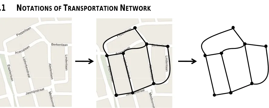
FIGURE 1: TRANSPORTATION NETWORK REPRESENTED AS A GRAPH

For studying the TAP, we need to introduce some notation. We consider a graph = ( , )

representing a transportation network, with nodes and links. The links represent roads, the set of links is denoted as and a link as . The nodes represent intersections of links. The set of nodes are denoted as and a node as . On the nodes we can define junctions. For a detailed explanation of junctions in the model, see Section 2.5. The traffic flow on the network is represented as load on the links, in vehicles per hour, denoted by . The cost of travelling experienced by the user is dominated by travel time. In our model other variables, such as distance and toll, are ignored, and we set the travel costs equal to travel time. We consider congested networks, this means when it gets busy on a road, the travel time increases. Therefore the travel time on link is a monotonically increasing function ( ), which we call the cost function of link . Later on, we will generalize the model by setting cost functions to ( ), where is a vector of all link loads = ( , ∈ ).

Een verkeersmodel is natuurlijk gebaseerd op een echt verkeersnetwerk, met wegen en kruispunten. We geven dit vereenvoudigd weer, de kruispunten zijn punten, daartussen lopen lijnen die de wegen weergeven, zie Figuur 1. Aan die lijnen (wegen) ‘hangen’ we een kostenfunctie, die berekent de reistijd, geven de hoeveelheid verkeer op de weg. Deze kostenfuncties zullen een centrale rol spelen in dit onderzoek.

There are several ways to define the cost function ( ). The conventional approach is the Bureau of Public Roads (BPR) function:

( ) = _max 1 + ,

(2.1)

where

is the length of link ;

max _{is the maximum speed on link ;}

is the load on link ;

is the capacity of link and

10

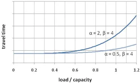
Note that _max corresponds to the ‘free flow travel time’, that is the travel time when there is no load on a link. is usually set on 4. The value of depends on the type of road. For highways a low value of is used, for example = 0.5, for urban roads usually a higher value of is used, for example

= 2. In Figure 2, the graphs of two BPR functions are shown.

FIGURE 2: GRAPH OF BPR-FUNCTION

Furthermore, notation with respect to paths, origins and destinations is needed. Travellers begin their journey at their origin, denoted by , and end at their destination, denoted by . The set of all origins is denoted by and the set of all destinations by , and is called an -pair. The set of all -pairs is denoted as . The demand is the amount of travellers that wants to travel from to , and is denoted by . A path from to is denoted by , the set of all paths from to is denoted by . All paths are in the set . Load is not solely defined on links, but also on paths. The relation between the link loads and path loads is given by the link-path incidence relationship

= _,

∈ ,

, _(2.2)

where

, =

1, if link is on path connec ng and ; 0, otherwise and is the load on a path connec ng and .

11

2.2

M

F

TAP

When choosing a specific TAP, one has to quantify a goal. That is, state some characteristics of the final flow on the road network. In traffic modelling, we want to assign traffic in a way that it approximates reality. We assume that in a realistic situation every traveller behaves independently and seeks to minimize his own travel time. Wardrop (1952) stated in his ‘first principal’ that this leads to User Equilibrium (UE), which means that traffic will distribute over the network in a way that no individual can decrease his travel time by changing his route. So our goal is to assign traffic such that UE is obtained.

We gaan ervan uit dat we in de verkeersmodellen een ‘gebruikersevenwicht’ moeten krijgen, een situatie waarbij niemand zijn eigen reistijd nog kan verkleinen. Wardrop heeft in 1952 al gezegd dat dit een realistische situatie is. We willen dat het verkeersmodel een realistisch verkeerspatroon geeft, dus we nemen gebruikersevenwicht als doel van de toedeling. In de formules hieronder wordt beschreven hoe je kunt controleren of de situatie een gebruikersevenwicht is. Eén van de dingen die bijvoorbeeld moet gelden is: als er verkeer over een route gaat, dan moet die route wel een optimale reistijd hebben, anders had niemand die route gekozen. En als er geen verkeer over een route gaat, dan moet die minstens zo lang duren als de optimale route, anders zou iemand die route wel gekozen hebben. Ook zijn er nog wat vanzelfsprekende eisen, zoals: er mag geen negatieve hoeveelheid verkeer over een route rijden.

UE is obtained, when a path flow solution ̅= ( ̅ , ∈ , ∈ ), satisfies the following Wardrop equilibrium conditions:

̅ _{̅ − = 0, ∀ ∈ , ∀ ; (2.3)}

̅ ≥ , ∀ ∈ , ∀ ; (2.4)

∑ ̅ = , ∀ ∈ , ∀ ; (2.5)

̅ _{≥0, ≥0, ∀ ∈ , ∀ , (2.6)}

where is the optimal travel time from to . This is also known as the complementarity problem.

Equation (2.3) has to hold at equilibrium because either a route has no load on it: ̅ = 0, or there is load on a route and the travel time of that route equals the optimal travel time: ̅ − = 0. Equation (2.4) holds at equilibrium because all routes from to have either the optimal travel time or the travel time is longer. Equation (2.5) concerns flow conservation, it ensures that the total flow from to always meets the demand. Finally non-negativity constraints (2.6) have to hold.

In the remainder of this section two mathematical formulations of the TAP are given, first as an optimization problem, then as a Variational Inequality Problem. Also, proofs are given that these formulations are equivalent, and that solutions to both formulations are UE flows.

2.2.1 OPTIMIZATION PROBLEM

12

The UE-based ‘Beckmann formulation’ of the TAP is as follows.

min ( ) =∑ ∫ ( ) , (2.7)

subject to ∑ = , ∀ ∈ , ∀ ; (2.8)

≥0, ∀ ∈ , ∀ ; (2.9)

=∑ _{, , ,} , ∀ . (2.10)

This optimization problem has an objective function ( ), see equation (2.7), which is nonlinear and convex, and the constraints are linear. Constraint (2.8) is the flow conservation constraint. Constraint (2.9) ensures that the load is positive. The link-path incidence relationship is added as a constraint (2.10). A solution is a certain traffic flow pattern, and is said to be feasible if it meets the constraints. The set of all feasible form the feasible region, which is a polyhedron on a hyper plane. The optimal solution ̅, which minimizes the objective function, is the flow pattern at user equilibrium. Actually, a solution to the Beckmann formulation is both an and an . We simply call ̅ user equilibrium when ( ̅, ̅) satisfies (2.8) – (2.10) and ̅ satisfies the Wardrop equilibrium conditions as stated in equation (2.3) – (2.6). Why ̅ is user equilibrium will be explained with an example in Section 2.2.1.1, and the proof will be given in Section 2.2.3.

Zo’n toedeling, hoe doe je dat eigenlijk? Hoe beschrijf je het als een opgave, of zoals wiskundigen zeggen liever ‘probleem’, en hoe los je het op? Beckmann beschreef het probleem in 1956 als een optimalisatie probleem. Hij gaf daarmee gelijk ook een hint voor het oplossen: optimaliseren zou moeten werken. Het optimalisatie probleem stelt dat er allerlei oplossingen zijn, maar dat er één optimale oplossing is. Met een oplossing bedoelen we een bepaald verkeerspatroon, bijvoorbeeld zeven mensen rijden linksom en twee mensen rijdt rechtsom, of ze rijden alle negen rechtsom. Er zijn vaak meerdere oplossingen die ‘kloppen’, dat betekent dat er aan eisen wordt voldaan zoals: iedereen komt vanuit zijn herkomst aan op zijn bestemming, er is geen negatieve hoeveelheid verkeer, etc. Maar welke van die ‘kloppende’ oplossingen is nu het gebruikersevenwicht waar we naar op zoek zijn? Die oplossing kun je krijgen door een bepaalde functie (vergelijking (2.5)) te minimaliseren. We noemen deze functie de doelfunctie. In deze functie wordt de oppervlakte onder de grafieken van de kostenfuncties gebruikt (zie Figuur 4). Om precies te zijn, als je de som van de oppervlakte onder de grafieken minimaliseert, dan vind je een situatie waarbij reistijden gelijk (en dus optimaal) zijn, en dat is het gebruikersevenwicht.

The objective function ( ) in the Beckmann formulation above is expressed in link flows, but via the link-path incidence relationship =∑ _{, , ,} , also a path flow solution can be obtained. Note that the path flow solution is not necessarily unique. The relation between link flows and path flows will be discussed in Section 2.6.

2.2.1.1 BECKMANN FORMULATION AND USER EQUILIBRIUM

In this example it is explained why minimizing the objective function ( ) =∑ ∫ ( ) of the Beckmann formulation yields user equilibrium.

FIGURE 3: EXAMPLE NETWORK

r

s

1

13 Let us consider the case of a simple network shown in Figure 3, with one origin , one destination , and two links between them. Assume the cost function of the links are: c = 10 + 3 and

c = 15 + 2 .

FIGURE 4: BECKMANN TRANSFORMATION AND USER EQUILIBRIUM

In Figure 4(A) the two cost functions are shown in one coordinate system. The load is shown on the -axis, where a point on the -axis is corresponding to a flow pattern. The sum of all loads meets the demand, that is + = . The load is shown from left to right, and the load is shown from right to left. For example, the left hand side of the x-axis corresponds to the case where all flow is send through link 2, and nothing through link 1. The cost functions are plotted. At user equilibrium the travel time on all used paths must be equal. This is at the intersection of the cost functions, marked as ‘user equilibrium’ in the figure. This intersection (and the corresponding flow pattern) is obtained by minimizing the surface under the graphs. Figure 4(B) shows that choosing a different flow pattern (represented by another value on the x-axis), yields a higher value of the surface under the graphs. Therefore, the minimization of the surface yields user equilibrium.

A formal proof of the equivalence of the Beckmann formulation and UE is given in Section 2.2.3.

2.2.1.2 USER EQUILIBRIUM VERSUS SYSTEM OPTIMUM

The Beckmann formulation of the TAP can be formulated for two purposes, to yield either a System Optimum (SO-based TAP) or a User Equilibrium (UE-based TAP). In the SO-based TAP the aim is to minimize the sum of all travel times, the solution is ‘optimal for the system’. Still, it is not necessarily optimal to an individual. In this example the difference between the SO and UE is explained.

Given the network presented in Figure 3, with demand = 12. First consider the UE solution. Substituting the cost functions in the Beckmann formulation yields to

min ( ) =∑ ∫ ( )

=∫ (10 + 3 ) +∫ (15 + 2 )

= 10 + + 15 + ,

subject to + = 12 ;

≥0, ∀ .

14

min ( ) = 10 + + 15(12− ) + (12− ) , ≥0, ∀ .

Differentiating ( ) and equate to zero, leads to the solution ̅ = 5.8 and ̅ = 6.2. Since this flow pattern is User Equilibrium, the travel time on both paths should be the same. We can check this, on both paths the travel time is 10 + 3∙5.8 = 15 + 2∙6.2 = 27.4. For comparison with the System Optimum described below, note that the total travel time is ̅ + ̅ = 5.8(10 + 3∙5.8) +

6.2(15 + 2∙6.2) = 328.8.

Now let’s consider the System Optimum in this network. In the System Optimum, the aim is to minimize the total travel time, so the optimization problem becomes

min ( ) =∑ ( )∙

= (10 + 3∙ ) + (15 + 2∙ )

= 10 + 3 + 15 + 2 ,

subject to + = 12 ;

≥0, ∀ .

Substituting = 12− in the above formulation yields to

min ( ) = 10 + 3 + 15(12− ) + 2(12− ) , ≥0, ∀ .

Differentiating ( ) and equate to zero, leads to the solution ̅ = 5.3 and ̅ = 6.7. Note that the travel times on both paths are different: = 10 + 3∙5.3 = 25.9 and = 15 + 2∙6.7 = 28.4. A traveler at path 2 could feel disadvantaged, knowing that travelling along path 1 is faster. Still, the total travel time of the system is ( ̅) = ̅ + ̅ = 5.3(10 + 3∙5.3) + 6.7(15 + 2∙6.7) =

327.55, and that is smaller than the total travel time in the User Equilibrium (where + =

328.8).

Summarizing, optimizing group performance usually results in different flow patterns and travel times than optimizing individual performance. It depends on the goal which model is used.

2.2.2 VARIATIONAL INEQUALITY PROBLEM

The Beckmann formulation of the TAP as discussed above, deals with costs = ( ) solely depending on the load on link . Generalizing, we can imagine cases where there is interaction of traffic between links, so the cost of a link also depends on load on other links in the network, for example at junctions or with two-way traffic. Then the cost function becomes non-separable, that is,

= ( ) where is a vector of all link loads = ( , ∈ ). In other words, the Jacobian of ( )

has zero off-diagonal entries. When junctions are modelled, some cost functions become non-separable, because the cost function of a turn also depends on the load on an conflicting turn.

15 switch to a generalized formulation of the optimization problem, namely the Variational Inequality Problem.

Mooi, dat optimalisatieprobleem van Beckmann, maar het blijkt niet altijd een toerijkende omschrijving. De doelfunctie die geminimaliseerd moet worden gebruikt de oppervlakte onder een grafiek, en die krijgen we door te integreren. Helaas kunnen we niet alle functies integreren, en dat is geen onvermogen, maar de integraal bestáát soms gewoon niet.

De functies die we zouden moeten integreren zijn de kostenfuncties, die voor elke weg een reistijd berekenen. Normaalgesproken is dat geen probleem, deze functies kunnen we integreren en we kunnen dus het optimalisatieprobleem van Beckmann gebruiken. Maar als de reistijd niet alleen bepaald wordt door het verkeer op de weg zelf, maar ook beïnvloed wordt door verkeer op andere wegen, zoals het geval is op kruispunten, dan zou dit wel eens problematisch kunnen worden... De kostenfuncties worden dan namelijk ‘niet-seperabel’, en als ze ook nog eens asymmetrisch zijn dan is integreren onmogelijk. Wat asymmetrie van een functie precies is is niet belangrijk voor het verhaal, zie het als een willekeurig kenmerk van de kostenfunctie.

Als integreren onmogelijk is bestaat de doelfunctie niet meer, en in dat geval zouden we over moeten stappen naar een algemenere formulering van de toedeling, namelijk de ‘variationele ongelijkheid’. Dafermos heeft in 1980 als eerste laten zien dat de toedeling ook zo omschreven kan worden. Die beschrijving van de toedeling als variationele ongelijkheid is lekker kort door de bocht: ‘Voldoet je oplossing aan deze ongelijkheid? Dan heb je de optimale oplossing gevonden!’. Zie vergelijking (2.12).

TEXTBOX 1: BECKMANN AND ASYMMETRICAL COSTS

In the objective function of the Beckmann formulation we look for a function ( ) such that

∇ ( ) = ( ).

THEOREM

Let ( ) be a twice continuously differentiable function. ( ) exists if and only if ∇ ( ) is symmetric.

PROOF

First we will proof: If ( ) exists → if ∇ ( ) is symmetric.

If ( ) exists then the following equation has to hold, obtained by differentiating both sides:

∇ ( ) =∇ ( ).

∇ ( ) is symmetric, because every Hessian is symmetric. Therefore, also ∇ ( ) has to be symmetric.

Second we have to proof: if ∇ ( ) is symmetric → ( ) exists. For this proof, we refer to ‘Poincaré’s Lemma’.

▪

16

In general, a VIP seeks a feasible solution ̅ ≥0 such that the following Variational Inequality (VI) holds:

∇ ( ̅)( − ̅)≥0, ∀ ∈feasible set. (2.11)

The TAP formulated as a Variational Inequality (VI) is: seeks a feasible solution ̅ ≥0 such that

( ̅) ( − ̅)≥0, ∀ ∈feasible set, (2.12)

where ( ) is a vector of all cost functions ( ) = ( ( ),∀ ∈ ). The solution ̅ is the optimal flow pattern, and corresponds to UE.

In the case of symmetric cost functions, it is proven that ̅ is the solution of the VI if and only if ̅ is the optimal solution of the Beckmann formulation. We will show this in the next section.

2.2.3 EQUIVALENCE PROBLEM FORMULATIONS AND USER EQUILIBRIUM

In this section a proof is given about the equivalence of the Beckmann transformation, the Variational Inequality formulation of the TAP and UE. An overview of the theorems is shown in Figure 5.

FIGURE 5: OVERVIEW THEOREMS

By introducing some new notation,

is the path-OD matrix, where an element _, = 1, if path ∈ ; 0, otherwise;

∆ is the link-path incidence matrix, where an element _, = 1, if link is on path ; 0, otherwise; is a vector of all path loads, that is = { ,∀ ∈ };

is a vector of all link loads, that is = { ,∀ ∈ };

is a vector of the demand, that is = { ,∀ ∈ },

we can rewrite the Beckmann transformation like this, under the assumption that ∇ ( ) = ( ),

min ( ) =∑ ∫ ( ) , (2.13)

subject to = , (2.14)

∆ = , (2.15)

− ≤0. (2.16)

The Lagrangian of this optimization problem is

x

x

x

x

2

3

1a

1b

17

( , , , , ) = ( ) + ( − ) + (∆ − )− , (2.17)

≥0, ≥0, (2.18)

where , , are Lagrange multipliers (also called dual variables), and have dimensions ∈ ℝ| |, ∈ ℝ| | and ∈ ℝ| |.

The optimizer of the optimization problem is denoted by ̅, and the corresponding dual parameters are denoted by , where = { , , }. As a property of the Lagrangian, the optimum is a saddle point of , that is, it is the minimum with respect to and maximum with respect to , so

( ̅, )≤ ( ̅, )≤ ( , ), ∀ , ∈feasible region. (2.19)

THEOREM 1

a) If is the optimal solution of the Beckmann transformation then it satisfies the KKT conditions.

b) If is convex and satisfies the KKT conditions then is the optimal solution of the Beckmann transformation.

PROOF OF 1A

A well known result from Karush, Kuhn and Tucker is that, under the slater condition, which are satisfied because the constraints are linear, at a minimum necessarily the first order conditions, called the Karush, Kuhn and Tucker (KKT) conditions, must hold:

= 0, (2.20)

= 0, (2.21)

= 0, = 1,2, (2.22)

= 0, ≤0, (2.23)

≥0. (2.24)

For the Beckmann transformation, these conditions are

=∇ ( )− = ( )− = 0, _(2.25)

=− +∆ − = 0, (2.26)

= 0, ≥0, (2.27)

≥0. (2.28)

PROOF OF 1B

A well known result from convex programming is: if the first order conditions hold, and z is convex, then we have obtained the optimum.

18

THEOREM 2

A feasible is a UE flow pattern if and only if satisfies the KKT conditions.

PROOF OF 2

We will show that we can rewrite the KKT conditions to UE.

We can rewrite equation (2.26) in the following way.

− +∆ − = 0, (2.29)

=∆ − , (2.30)

Using condition (2.25), we can rewrite this as

=∆ ( )− . (2.31)

Because of condition (2.27) and (2.28)

= = 0, if > 0;

≥0, if = 0. (2.32)

Also, the link costs are transformed into path costs using

∆ ( ) = ( ). (2.33)

Using (2.32) and (2.33) in equation (2.31), we obtain

=∆ ( )− = ( )− (2.34)

Recall an entry in is 1 if path is connecting -pair . Because a path can only connect one OD-pair, but an OD-pair can be connected by more paths, ∈ ℝ| |×| | has the form:

=

⎣ ⎢ ⎢ ⎢ ⎢

⎡1₁ 0 0_{0 0}

0 1 0

0 1 0

⋯ 0

⋮

0

⋱ 1

0 1⎦

⎥ ⎥ ⎥ ⎥ ⎤

For a specific and ∈ , equation (2.34) is

= [∆ ( )] − = ( )− = = ( ), if > 0;

≤ ( ), if = 0. (2.35)

This is exactly UE, since the costs of a path are equal for all used paths, and an unused path has equal or higher costs.

▪

THEOREM 3

The feasible ̅ is a solution of the Variational Inequality formulation of the TAP if and only if the feasible ̅ is a User Equilibrium.

PROOF OF 3

First we will proof that: ̅ is UE → ̅ is solution of VI.

If is UE, with corresponding ̅ the equilibrium conditions hold

19

̅ ≥ , ∀ ∈ , ∀ ; (2.37)

∑ ̅ = , ∀ ∈ , ∀ ; (2.38)

̅ _{≥0, ≥0. (2.39)}

Also, the constraints hold

∑ ̅ = , ∀ ∈ , ∀ ; (2.40)

̅ _{≥0, ∀ ∈ , ∀ ; (2.41)}

̅ =∑ _{, , ,} ̅ , ∀ . (2.42)

From equations (2.36) and (2.37) and (2.39), we know

̅ − ≥0. (2.43)

Subtracting (2.36) from (2.43) we obtain:

− ̅ ̅ − ≥0, (2.44)

̅ _{− ̅ − − ̅ ≥0. (2.45)}

Summing over paths yields

̅ − ̅

,

− − ̅

,

≥0, _(2.46)

̅ − ̅

,

− − ̅ ≥0. _(2.47)

From flow conservation constraint (2.38) the latter term vanishes, therefore

̅ − ̅

,

≥0. _(2.48)

This is the Variational Inequality formulation, with respect to , namely

̅ _{− ̅ ≥0, ∀ feasible .} (2.49)

For the proof that: ̅ is solution of VI → ̅ is solution of Beckmann transformation, we refer to Florian and Hearn (1995). From Theorem 1a and Theorem 2 we know that if ̅ is solution of Beckmann transformation, then ̅ is UE. This completes the proof.

20

2.3

E

U

In this section, the TAP is considered with respect to the existence and uniqueness of solutions.

In the case of TAP with separable costs, Beckmann et al. (1956) showed that if the cost function is monotonically increasing function of , the optimal solution is unique, and is obtained by solving an optimization problem as in equations (2.7) – (2.10).

When adding junction delays to the TAP, the cost functions become non-separable. Considering the Jacobian of the cost function,

= , (2.50)

non-separable costs yields non-zero off-diagonal entries. The Jacobian has several properties, can be symmetrical, that is

= , ∀ , (2.51)

and can be diagonally dominant, that is

≥ , ∀ (row dominance), _(2.52)

and ≥ , ∀ (column dominance). _(2.53)

Note that a diagonal dominant Jacobian implies a positive semi-definite Jacobian. A matrix is positive semi-definite if

≥0, ∀ ≠0. (2.54)

A positive semi-definite Jacobian is a sufficient condition for convexity of the problem. Dafermos (1971) showed that if the Jacobian is symmetric and positive definite, the TAP has a unique solution which is obtained by a minimization problem. Later Dafermos (1980) showed that the TAP can also be expressed as a VIP, and she showed that also in the case of an asymmetric Jacobian the solution of the VIP is globally unique, under the assumption of a globally positive definite Jacobian. Diagonally dominance is a stronger criterion for the existence of a unique solution.

21 In a realistic transportation network, taken junctions into account, in general the cost functions are non-separable, the Jacobian is asymmetric and the Jacobian may be non-diagonally dominant. Consider for example a priority junction. The influence of a major road (priority) on a minor road (no priority) is not equal to the influence of a minor road on a major road, and therefore the cost functions are asymmetric. Further, the cost function on a turn from a minor road crossing a major road can be dominated by the load on the major road instead of the load on the minor road itself. In this situation the cost function is non-diagonally dominant.

Therefore, when junction delays are modelled realistic, non-diagonally dominant cost functions exist, and a unique solution is not guaranteed. This means that, in reality, multiple equilibrium solutions may exist, which corresponds to different traffic flow patterns.

Als we kijken naar de reistijd (of beter gezegd: vertraging) die opgelopen wordt op kruispunten in de realiteit, dan wordt deze enerzijds beïnvloed door de hoeveelheid verkeer op de weg waar je zelf op rijdt. Hoe drukker het is in ‘jouw’ verkeersstroom, hoe langer je bij een kruistpunt staat te wachten. Anderzijds wordt de vertraging ook bepaald door de hoeveelheid verkeer op andere wegen. Hoe drukker het is op de kruisende verkeersstromen, hoe langer je staat te wachten. Sterker nog, er zijn voldoende situaties denkbaar, bijvoorbeeld op voorrangskruispunten, waarbij de kruisende verkeersstroom een grotere invloed heeft op de vertraging dan je eigen verkeersstroom. Dit betekent in wiskundige termen dat de kostenfunctie niet-diagonaal dominant is.

Dit betekent dat er in de realiteit geen unieke oplossing is gegarandeerd, en kunnen meerdere gebruikersevenwichten bestaan, verschillende verkeerspatronen waarin toch niemand zijn reistijd kan verkleinen.

One can question the goal of modelling traffic. Should the model approach reality as close as possible, even if it adopts the existence of several equilibria? That would imply that the model could result in different flow patterns, depending on for example its initialization or the solving method. In that case the given solution is not necessarily the same as the real situation, since there are more solutions. Also when comparing different scenarios, a fair comparison could be problematic. For these reasons, one can state it is better for the model to always converge to the same unique solution. But on the other hand, when a unique solution is required, convexity of the problem is needed. That implies no non-diagonal dominant turn costs are accepted, and that is not always realistic. Concluding, if one states the turn costs must be as accurate as possible, one has to take the existence of several local minima for granted.

22

2.4

O

TRANS

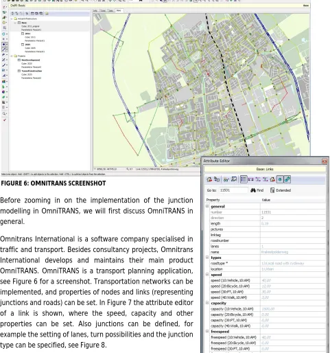
Before zooming in on the implementation of the junction modelling in OmniTRANS, we will first discuss OmniTRANS in general.

Omnitrans International is a software company specialised in traffic and transport. Besides consultancy projects, Omnitrans International develops and maintains their main product OmniTRANS. OmniTRANS is a transport planning application, see Figure 6 for a screenshot. Transportation networks can be implemented, and properties of nodes and links (representing junctions and roads) can be set. In Figure 7 the attribute editor of a link is shown, where the speed, capacity and other properties can be set. Also junctions can be defined, for example the setting of lanes, turn possibilities and the junction type can be specified, see Figure 8.

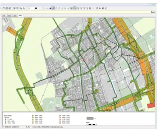
In OmniTRANS an assignment can be executed. The solution can be visualized, by ‘plotting’ the load on the network. An example is shown in Figure 9. The colour and the thickness of the links represent selected information, for example the load, the costs or the load / capacity ratio. Using this visualization, congestion and bottlenecks can easily be examined.

FIGURE 6: OMNITRANS SCREENSHOT

23

FIGURE 8: JUNCTION EDITOR

24

2.5

J

M

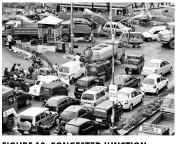
In congested urban networks, relatively much of the time spent on a journey is incurred by queuing and turning at junctions. In most traffic models junction delays are ignored, or average delays are used. For highway modelling, still accurate solutions are obtained, but in urban networks the lack of accurate junction delays in the model can lead to significant errors. To illustrate the importance of the contribution of junction delays to the total travel time, see Figure 10. No one would easily ignore the delay at this junction when calculating the travel time of a route passing this junction.

FIGURE 11: EXPANDED JUNCTION

A common way to model junctions in a network, is to expand the junction nodes. All possible turns become extra links and all branches of the junction get a node. An example of an expanded junction with four branches is shown in Figure 11. On each turn a cost function is defined, which is a function of the load on the turn itself and the load on conflicting turns. In the next section an explanation is given of the specific junction modelling in OmniTRANS.

Bij de toedeling spelen reistijden een belangrijke rol. We ‘zoeken’ immers naar een situatie waarin alle reizigers een minimale reistijd ervaren van hun herkomst naar hun bestemming. Een goede en waarheidsgetrouwe berekening van de reistijden is dus van groot belang. In stedelijke verkeersnetwerken wordt een groot deel van de reistijd over de hele route opgelopen bij kruispunten. Het is daarom belangrijk dat de kruispuntvertragingen accuraat meegenomen worden in de berekening van de reistijden.

In de meeste verkeersmodellen wordt de kruispuntvertraging genegeerd, of wordt er gewerkt met vaste waardes voor kruispuntvertragingen, ongeacht de drukte op een kruispunt. Echter, OmniTRANS gebruikt een hele uitgebreide module voor de kruispuntmodellering, die gegeven de hoeveelheid verkeer op de eigen en kruisende verkeersstromen een vertraging berekent in seconden. De berekeningen die hiervoor gemaakt worden staan beschreven in paragraaf 2.5.2. Hoe ‘zitten’ deze kruispuntvertragingen eigenlijk verwerkt in het verkeersmodel? We hebben eerder gezien dat er aan wegen een kostenfunctie werd ‘gehangen’, die gegeven de hoeveelheid verkeer de reistijd berekende. Hetzelfde doen we voor ‘turns’, dat zijn afslagbewegingen op een kruispunt. Turns worden gerepresenteerd als een lijn in het netwerk, zie Figuur 11. Aan elke turn wordt ook een kostenfunctie ‘gehangen’, die de vertraging voor die turn geeft.

25 2.5.2 JUNCTION MODELLING IN OMNITRANS

OmniTRANS contains an extensive junction modelling module, where all types of junctions can be defined, namely equal junctions, priority junctions, signalized junctions and roundabouts. Also, a number of lanes on every branch of the junction and possible turning movements on those lanes can be defined, see Figure 12 for some examples. Calculations are made per lane, per turn, or per lane

group. A lane is a road section used for a turn or a combination of turns. Turns are movements of one branch to another, possible turns are left, through and right. Lane groups are circled in Figure 12. Note that if more turning movements are possible from one lane, the turning movements are in the same lane group. Also, if the same turning movement can be made from different lanes, those lanes are in the same lane group.

Generally, the capacity is calculated per lane group and the delay is calculated per lane. In the formulas the lanes are denoted by , the lane groups are denoted by and the turns are denoted by . The calculation of the capacity and the delay differs per junction type, the main differences are between signalized and unsignalized junctions. Besides capacity and delay, also the setting of traffic lights are (optionally) calculated in OmniTRANS. In the next sections, the main calculations are given.

For clearness, these calculations are simplified in a sense that all the parameters are omitted. We maintain the ´structure´ of the formulas, in a way that it is workable and relevant for our purposes. For a complete overview of the calculations in junction modelling in OmniTRANS, see the documentation of OmniTRANS ‘Explanation of Junction Modelling’ (Brandt & Schilpzand, 2007). These calculations are partially based on the formulas for capacity and delay in the Highway Capacity Manual (Transportation Research Board, 2000).

Next to omitting parameters, also a variable is omitted, namely the ‘apparent conflict’ variable. Apparent conflicts are situations where a driver unnecessary waits for another driver. This could happen for example when driver A wants to enter a roundabout, but is waiting for driver B, who is going to exit the roundabout. Driver B forgot his turning signal, so actually there is no conflict, but still driver A experiences a conflict situation and is waiting unnecessarily for driver B. In this study no apparent conflicts, but only real conflicts are taken into account.

First the calculations of capacity and delay of unsignalized junctions are discussed. Thereafter, the calculation of a signalized junction, including the setting of traffic lights, is discussed. Finally, a general cost function of a turn is given.

(A)

(E) (D)

(C) (B)

26

2.5.2.1 UNSIGNALIZED JUNCTIONS CAPACITY

The calculation of the capacity of a lane group at an unsignalized junction is as follows

=max − ∑ _∈ , _min , (2.55)

where

is capacity of lane group ; is saturation flow;

is load on lane group ;

is set of lane groups conflicting with lane group and

min is minimal capacity of lane group .

The saturation flow is the capacity when there are no conflicting movements. The minimal capacity is used to avoid total congestion.

The calculation of the capacity at a priority junction is extended with some extra terms. Those terms provide the decrease of the capacity as a result of the difficulty of crossing a priority junction for a minor road. Those terms are fixed values for every junction, and therefore omitted.

The delay depends on the capacity. The delay is calculated per lane, whereas the capacity is calculated per lane group. We can obtain the capacity per lane by dividing the capacity of the lane group proportionally over the lanes. For the complete calculation, see Brandt and Schilpzand (2007).

DELAY

The general formula for the delay (cost function) at an unsignalized junction is as follows

= min _, + _, + _, , _, , (2.56)

where

is average delay on lane ; , is uniform delay on lane ; , is incremental delay on lane ; , is geometric delay on lane and

, is maximal delay on lane .

, is used to avoid total congestion.

The uniform delay _, and the incremental delay _, are calculated as follows

, =

1

, (2.57)

, =

⎩ ⎪ ⎨ ⎪ ⎧

−1 + −1 +

( ) , if > ;

0, if ≤ ,

27 where

is load on lane ; is capacity of lane and

is a parameter usually set on 0.5.

Both uniform delay and incremental delay are proportional with the load on the lane , and inversely proportional with the capacity . Note that the incremental delay is only taken into account when the ratio ⁄ is greater than , which is usually 0,5.

The geometric delay , is calculated per junction type as follows:

equal junction: _, = 1, if > 0;

0, if = 0, (2.59)

priority junction: _, =

1, if > 0 and branch is major road;

adjusted

,if > 0 and branch is minor road;

, if = 0,

(2.60)

unsignalized roundabout: , = , (2.61)

where

adjusted= left+ through+ right , with left is load on left turn movements, through is load on through movements, right is load on right turn movements; is load on lane ;

is usually set on 7.

Note that in the adjusted load _adjusted the load on left and right movements have a greater weight than the trough movement.

Considering the Traffic Assignment Problem, the cost function of a turning movement at a junction is relevant. Generally, the cost function is a monotonically increasing function of the load on its own turning movement and the load on conflicting movements. The influence of the load on the conflicting movements is via the capacity: when load on conflicting movements increases, the capacity decreases, and therefore the cost function increases.

2.5.2.2 SIGNALIZED JUNCTION

28

CAPACITY AND SETTINGS OF TRAFFIC LIGHTS

The calculation of the capacity at a signalized junction is done as follows. First, the capacity of a turn is set on the saturation flow,

= , (2.62)

where

is base capacity of turn and is saturation flow of turn .

Then the capacity per lane is calculated from the capacity per turn as follows,

=∑ on lane

ℎ , (2.63)

where

is base capacity of lane and ℎ is number of turns on lane .

Naturally the final capacity of a lane depends on the green time, which is the period the traffic light is green for that lane, so that the travellers can pass the junction. The green time is the same for all lanes in one lane group. For calculating the green time, information is needed about the conflicting lane groups. A conflict matrix is used, where conflicts between all pairs of lane groups are given. Then ‘maximum conflict groups’ are obtained, these are maximum groups consisting of lane groups which are in conflict with all the other lane groups in the group. For every conflict group, the signal cycle time is calculated, it is set on the minimum time period such that the junction can ‘digest’ all the traffic in the conflict group. The normative conflict group is the conflict group with the highest signal cycle time. This cycle time is used for the junction. This is limited by a maximum cycle time, to avoid a very high value. Then the green times of the lane groups are calculated. First the green times of the normative conflict group are calculated, thereafter the green times of the other conflict groups. For a more specific explanation of the calculation of conflict groups, cycle times and green times, see Brandt and Schilpzand (2007).

The final capacity of a lane is the base capacity times the fraction of green time the lane gets, that is

= , (2.64)

where

is capacity of lane ;

is fraction green time of lane of total cycle time and is base capacity of lane .

DELAY

29

= min _, + _, + _, , _, , (2.65)

where

is average delay on lane ; , is uniform delay on lane ; , is incremental delay on lane ; , is geometric delay on lane and

, is maximal delay on lane .

At a signalized junction uniform delay , is calculated as follows

, = ∙

(1− )

1−min 1, ∙ , (2.66)

where

is fraction green time of lane of total cycle time; is cycle time;

is load on lane and is capacity of lane .

For explaining how is calculated, we need to introduce phases, which we denote by . The cycle time consists of phases, and a phase is a time period where a set of lanes gets green. is the set of lanes that get green in phase . The fraction of green time of lane is calculated as follows

=

max ∈

∑ max

∈

, (2.67)

where

is load on lane ;

is base capacity of lane and

is the set of lanes that get green in phase .

This can be interpreted as follows. In a certain phase the lane with the highest load / capacity ratio is obtained. The proportion of this load / capacity ratio of the sum of all maximum load / capacity ratios of all phases, is the proportion of green time it gets. So green times are proportionally divided based on the maximum load / capacity ratio of all the phases.

The incremental delay _, is calculated in the same manner as at an unsignalized junction, so

, =

⎩ ⎪ ⎨ ⎪ ⎧

−1 + −1 +

( ) , if > ;

0, if ≤ ,

(2.68)

where

30

The geometrical delay _, is calculated roughly the same way as at an unsignalized junction,

, =

adjusted

, if > 0;

, if = 0,

(2.69)

where

adjusted= left+ through+ right , with left is load on left turn movements, through is load on through movements, _right is load on right turn movements;

is load on lane and is usually set on 7.

Concluding, as at an unsignalized junction, also at a signalized junction the cost function is a monotonically increasing function of the load on its own turning movement and the load on conflicting movements, although the cost function is slightly different.

2.5.2.3 COST FUNCTIONS FOR A TURN AT A JUNCTION

For simplicity, we assume that every lane corresponds to one turn, see Figure 12(D), we omit the minimal capacity, the maximal delay and the geometric delay ( , ).

Wat we vooral van deze berekeningen kunnen leren is dat de kruispuntvertragingen heel precies worden berekend. En hieronder staat dan dé kostenfunctie voor een ongeregeld kruispunt (vergelijking (2.70)) en voor een geregeld kruispunt (vergelijking (2.71)). Hoewel deze sterk vereenvoudigd zijn, is de ‘structuur’ van de functies behouden, zodat we deze exemplaren kunnen gebruiken om te kijken of ze voldoen aan de eisen voor een goede toedeling.

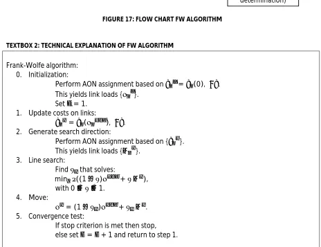
In total, the simplified cost function for a turn on a unsignalized junction is as follows.

= _, + _,

= 1 + −1 + −1 +

( )

= 1

− ∑ _∈ + − ∑ _∈ −1 + − ∑ _∈ −1 + _{− ∑}

∈

.

(2.70)

The simplified cost function for a turn on a signalized junction is

= _, + _, + _,

= ∙ (1− )

31

= ∙ (1− )

1−min 1, ∙ + −1 + −1 +( ) . (2.71)

where

is cost function (delay) on turn ; , is uniform delay on turn ; , is incremental delay on turn ; , is geometric delay on turn ; is capacity on turn ;

is saturation flow on turn ; is load on turn ;

is set of turns conflicting with turn ;

is fraction of green time of turn of total cycle time and is cycle time.

Note that when the signalized junctions are specified ‘manual’, and are fixed. When the signalized junctions are specified ‘automated’ or ‘actuated’, is a monotonically decreasing function of , because the more load on the conflicting movements, the less percentage of green time the total turn gets:

= =

max ∈

∑ max

∈

=

max ∈

max

∈ +∑ where gets green max∈

, (2.72)

where

is load on lane ;

is base capacity of lane ;

is the set of lanes that get green in phase and lanes are denoted by and .

Because all lanes get green in another phase as lane , lane is in conflict with lane by definition. So load , where ∈ , is in conflict with lane , where is the set of conflicting loads with lane .

Concluding, the cost function of a turn at a junction is, at both unsignalized and signalized junctions, a monotonically increasing function of the load on its own turning movement and the load on conflicting movements , where ∈ .

32

2.6

T

N

There are several interpretations when adding turns, with its load and cost, to a network. As we have seen in Section 2.5 in OmniTRANS the addition of turns is implemented as an extension of the network. The junctions are expanded, all turns become extra links and every branch of a junction gets a node, see Figure 11. Implemented in this manner, the solution of the assignment directly provides turn loads and costs.

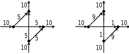
Considering the addition of turns to the network, naturally a question rises, namely can we construct the turn loads from the link loads? Although this is not relevant for OmniTRANS, it is still an interesting issue.

FIGURE 13: JUNCTION WITH UNKNOWN TURN LOADS

For example, in the junction in the Figure 13, the link loads are given. Ten travellers are approaching the junction from the West, ten from the South. Furthermore, ten travellers are leaving the junction to the North, and ten to the East. Can we determine how many travellers making specific turns, such that load fits with the link loads? There are multiple feasible solutions to this problem, two solutions of this instance are shown in a schematic representation in Figure 14.

FIGURE 14: POSSIBLE SOLUTIONS FOR TURN LOADS

A way to construct turn loads from link loads is via the path solution. In a path solution, the variables are paths instead of links and so the loads and costs are calculated per path. Therefore, the portion of travellers from one link to another is known, and the turns loads can be extracted.

2.6.1 FROM A LINK SOLUTION TO A PATH SOLUTION

As discussed in Section 2.2.1, the link solution and path solution are related by the link-path incidence relationship

=∑ _{, , ,} , (2.73)

where

10

10

10

10

10

10

10 10

10

10

10 5 5 10

5 ₅ 1 ₉

33 is the load on link ;

is the load of path connecting and ;

, =

1, if link is on path connec ng and and

0, otherwise.

Although a path solution uniquely determines a link solution, this does not hold for the reverse. Given a link solution, the path solution is not unique. And also, as shown in Figure 14, given a link solution the turn loads are not uniquely defined. This becomes more clear in the following two examples.

In example 1, a network is shown with one OD-pair, one junction and four possible routes. Given the link solution, two possible path solutions are given, in such a way that the link-path incidence relationship holds. Next to the path solution, the resulting turn loads on the junction are given. Example 2 contains an other network, with two OD-pairs, two junctions and two possible routes per OD-pair. Also two path solutions and the resulting turn loads on the left junction are given.

EXAMPLE 1:MORE PATH SOLUTIONS GIVEN A LINK SOLUTION

Network with link solution

= 20

Expanded junction

Path solution 1(a) With turn loads

Path solution 1(b) With turn loads

r s

10

10 10

10

r

10

10

0 0

r

r

r

s s

s s

0

10 10

0

r

5

5

5

5

r

r

r

s s

s s

5

5 5

34

EXAMPLE 2:MORE PATH SOLUTIONS GIVEN A LINK SOLUTION

Network with link solution

= 10_{= 20}

Expanded (left) junction

Flow solution 2(a) With turn loads

on left junction

Flow solution 2(b) With turn loads

on left junction

Considering the fact that a link solution does not uniquely determine a path solution, and thus turn loads, we can state that, given a link solution, a path solution has to be chosen according to some strategy. Naturally, we search for the ‘most likely’ path solution, given the link solution.

2.6.2 MOST LIKELY PATH SOLUTION

Larsson, Lundgren, Rydergren and Patriksson (2001) studied most likely path flows, given a link flow solution. They state that travellers are indifferent to which route they use, among all equal cost routes. Therefore, all route choices are equally probable. Using general principles from information theory, the most likely path solution is the one with the highest entropy.

The entropy value is, by definition,

− ln

∈

, _(2.74)

where is the load of path connecting and .

r s

20 10

20 10

p 9 q

21

11

p _q

s r

s r

q p

9 0 10

10

0 11

9

14

p _q

s

r

s

r

q p

6 3 7

7

3 14

35 A solution with a maximum, or ‘sufficiently high’, entropy value is also referred to as a path proportional solution.

To illustrate the meaning of the entropy value, the entropy value is calculated for the two examples above. In example 1, the entropy value for path solution 1(a) is

− ∑ ∑ _∈ ln = 2(10∙ln 10) + 2(0∙ln 0)≈ −46.05,

and the entropy value for path solution is 1(b) is

− ∑ ∑ _∈ ln = 4(5∙ln 5)≈ −32.19.

In example 2, the entropy value for path solution 2(a) is

− ∑ ∑ _∈ ln = 10∙ln 10 + 0∙ln 0 + 11∙ln 11 + 9∙ln 9≈ −69.18,

and the entropy value for path solution is 2(b) is

− ∑ ∑ ∈ ln = 7∙ln 7 + 3∙ln 3 + 14∙ln 14 + 6∙ln 6≈ −64.61.

The path solution of 1(b) and 2(b) has a higher entropy value than respectively the path solution of 1(a) and 2(a). These path solutions are indeed more likely path solutions, because the loads are more equally distributed over all possible paths.

The problem of finding the most likely path solution given a link solution, is the maximum entropy problem, which is as follows

max − ∑ ∑ _∈ ln , (2.75)

subject to ∑ _∈ = , ∀ ; (2.76)

∑ _{, , ,} = , ∀ ; (2.77)

≥0, ∀ , ∀ ∈ , (2.78)

where

is the load on link ;

is the load of path connecting and ;

, =

1, if link is on path connec ng and ; 0, otherwise, and is the demand from to .

In the maximum entropy problem the entropy value is maximized under the equilibrium constraints and the link-path incidence relationship. This is a strictly convex problem. Note that is the given link solution, and therefore is an input parameter.

Several solution methods of the maximum entropy problem are given by Larsson et al. (2001). Also Freund and Saxena (1984) give a solution method, the complexity of this algorithm is in order ( ), where is the number of paths.

36

37

2.7

F

P

F

Our problem is the static user equilibrium-based Traffic Assignment Problem with deterministic route choice, which we referred to as TAP, expanded with junction delays. In this section an overview is given of all implications of the addition of junction delays, as implemented in OmniTRANS, to the TAP.

We hebben in Hoofdstuk 2 bekeken wat voor soort probleem de toedeling eigenlijk is, hoe kruispuntmodellering dat kan beïnvloeden, en hoe kruispunten gemodelleerd zijn in OmniTRANS. In deze laatste paragraaf komt dat samen en presenteren we een uiteindelijke probleem formulering.

(NON-)SEPARABLE COST FUNCTIONS

When adding junction delays to the TAP, the nodes are expanded, and all turns become extra links, as we have seen in Section 2.5. On all links, both ‘normal’ links (representing roads) and ‘turn’ links (representing turns) a cost function is defined. The cost function of a ‘normal’ link is the BPR function

( ) = _max 1 + , (2.79)

the simplified cost function of a ‘turn’ link is, in the case of an unsignalized junction

( ) = 1

− ∑ _∈ + − ∑ _∈ −1 + − ∑ _∈ −1 + _{− ∑}

∈

, (2.80)

and in the case of a signalized junction

( ) = ∙ (1− )

1−min 1, ∙

+ −1 + −1 +

( ) ,

where

(2.81)

is the cost function (delay) on link ; is the length of link ;

max _{is the maximum speed on link ;} is the load on link ;

is the set with links conflicting with ; is the capacity of link ;

and are constants defined for every link; is the saturation flow;

is the load on conflicting movements with link ;

is fraction green time of link of total cycle time (we assume this to be fixed) and is cycle time (we assume this to be fixed).

38

vertraging niet alleen afhankelijk is van de eigen verkeersstroom, maar ook van de conflicterende verkeersstromen. We noemen deze kostenfuncties niet-seperabel.

The cost function of ‘normal’ links and the cost function of a turn at a signalized junction (assuming a fixed setting of traffic lights) are separable. Only the cost function of a turn at an unsignalized junction is non-separable, meaning that the delay depends on the load on the turn itself and also on the loads of conflicting turns.

DIAGONAL DOMINANCE

We know from Section 2.3 that, if the cost function is global diagonally dominant, we can guarantee there exists a globally unique equilibrium solution.

We zagen al eerder in paragraaf 2.3 dat als de kostenfunctie niet-diagonaal dominant is, dat we geen unieke oplossing kunnen garanderen. Ook constateerden we dat een realistische kruispuntvertraging inderdaad niet-diagonaal dominant is, omdat er situaties denkbaar zijn waarin de conflicterende verkeersstroom meer invloed heeft op de vertraging dan de eigen verkeersstroom. We kunnen nu verder nog stellen dat de kruispuntmodellering zoals die is geïmplementeerd in OmniTRANS ook niet perse diagonaal dominant is, en dat we het bestaan van meerdere gebruikersevenwichten in de verkeersmodellen in OmniTRANS dus niet kunnen uitsluiten.

Recall that diagonal dominance means

≥ , ∀ (row dominance), _(2.82)

and ≥ , ∀ (column dominance). _(2.83)

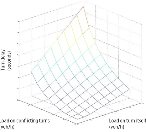
For inspecting the cost function of an unsignalized junction with respect to its diagonal dominance, we first extend the function with all the (relevant) parameters,

( ) = 3600

0,8 −0,99∑ _∈ +

900

⎝ ⎜ ⎜ ⎛

0,8 −0,99∑ _∈ −1

+ ⎷ ⃓ ⃓ ⃓ ⃓ ⃓ ⃓ ⃓ ⃓ ⃓

0,8 −0,99∑ _∈ −1 + 0,5

⎝ ⎜

⎛0,8 −0,99∑ _∈

0,8 −0,99∑ _∈

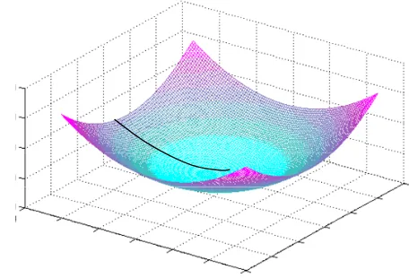
⎠ ⎟ ⎞ ⎠ ⎟ ⎟ ⎞ . (2.84)

This function is plotted in Figure 15, the and axis are respectively the load on the turn itself and the load on all the conflicting turns ∑ _∈ . The load is measured in vehicles per hour, and