Cost and Emissions Implications of Coupling Wind and Solar Power

Cost and Emissions Implications of Coupling Wind and

Solar Power

Seth Blumsack, Kelsey Richardson

John and Willie Leone Family Department of Energy and Mineral Engineering, Pennsylvania State University, University Park, USA.

Email: [email protected]

Received July 11th, 2012; revised August 22nd, 2012; accepted August 30th, 2012

ABSTRACT

We assess the implications on long-run average energy production costs and emissions of CO2 and some criteria pol-

lutants from coupling wind, solar and natural gas generation sources. We utilize five-minute meteorological data from a US location that has been estimated to have both high-quality wind and solar resources, to simulate production of a coupled generation system that produces a constant amount of electric energy. The natural gas turbine is utilized to pro- vide fill-in energy for the coupled wind/solar system, and is compared to a base case where the gas turbine produces a constant power output. We assess the impacts on variability of coupled wind and solar over multiple time scales, and compare this variability with regional demand in a nearby load center, and find that coupling wind and solar does de- crease variability of output. The cost analysis found that wind energy with gas back-up has a lower levelized cost of energy than using gas energy alone, resulting in production savings. Adding solar energy to the coupled system in- creases levelized cost of energy production; this cost is not made up by any reductions in emissions costs.

Keywords: Wind Energy; Solar Energy; Air Emissions

1. Introduction

The integration of renewable electric generation re- sources, particularly solar and wind, into existing energy production and delivery systems, is considered to be a major technical and economic challenge. Variability of both wind and solar resources introduces additional sto- chastic components to the operational objective of bal- ancing supply and demand across power control areas on a real-time basis; and presents planning challenges to system operators and generating companies that must make investment portfolio decisions to accommodate increased renewable energy penetration. Integration costs are expected to rise along with penetration levels, with recent reports suggesting costs of $2/MWh to $9/MWh [1] once wind penetration reaches 20% [2].

A number of different operational strategies are possi- ble to achieve large-scale penetration of wind and solar energy. One such strategy would expand the use of fre- quency regulation and balancing energy services to compensate for unforecasted deviations in wind and solar power output. These so-called ancillary services are cur- rently utilized in large-scale electricity systems to bal- ance unexpected deviations in the supply-demand bal- ance caused by volatile electricity demand or unplanned outages at generation or transmission assets. Such ancil-

lary services can be provided on the supply side or the demand side. While system operators are experienced in procuring and dispatching ancillary services to handle fluctuations in the supply-demand balance, it is less clear whether existing ancillary services, and the various types of markets through which they are procured, are adequate to support the large-scale integration of wind and solar resources while maintaining high reliability and reason- able costs [3].

ergy storage that compensate for “fast” energy storage [5].

The increased use of ancillary services versus the cou- pling of variable and controllable resources is an unset- tled topic in the electric utility industry and in the rele- vant research literature. We choose to assess the direct coupling of variable and controllable resources; in par- ticular we assess how coupling multiple variablere- sources affects the utilization of the controllable resource. Specifically, we compare the costs and emissions of two coupled energy systems with a base-case system feature- ing a natural gas combustion turbine that produces a con- stant amount of electric energy. For comparison, we cou- ple the natural gas turbine with an equivalently-sized wind energy installation; as well as coupling the gas tur- bine with a wind energy installation and a solar photo- voltaic installation. Differences in the diurnal cycles of wind and solar energy [3] suggest that coupling these two variable sources may reduce the utilization of the con- trollable (and polluting) energy resource, with concomi- tant benefits in terms of air emissions.

The remainder of the paper discusses our data sources, modeling strategy and results. Section 2 outlines the data we have obtained for a high-quality wind and solar site in western Oklahoma, and describes how we estimate wind and solar production based on meteorological data. Technology and emissions costs are also discussed in Section 2. Section 3 contains the results of our modeling exercise, and Section 4 offers some discussion and con- clusions.

2. Data and Modeling

Our case study is based on simulation of a coupled system of wind, solar and natural gas installed in Weatherford, in western Oklahoma. Weatherford is considered an advan- tageous location for such a coupled system since it is located in a high-quality wind zone (Class IV wind site [6]) and has relatively high-quality photovoltaic potential (based on analysis in [7]). We collect five-minute mete- orological data for the Weatherford location from the Oklahoma Mesonet, a collection of over one hundred measurement stations across Oklahoma. Data available through the Mesonet includes averages of five-minute wind speed (m/s), wind direction, average solar radiation

(W/m2), and other weather variables. Data are recorded at

a height of 10 m. We use 2002 as our study year, since that year is considered to be a historically average wind and solar irradiance year for Oklahoma.

2.1. Wind Power Modeling

Five-minute wind speed data at 10 m are converted to 80 m hub height data using the power-law equation:





V V H H (1)

where V1,t and V2,t are the recorded and estimated wind

speeds (m/s) at time interval t, at heights H1 and H2 (so in

our case, H1 = 10 m and H2= 80 m; V1,t represents the

time series of wind speeds that we obtained from the

Oklahoma Mesonet; and V2,t represents the estimated

time series of wind speeds). As a robustness check, we generated estimated wind speeds using the roughness equation:



 







2,t 1,t ln 2 ln 1 ,

V V H l H l (2)

where l is the roughness length. We do not have explicit

data on the roughness length for our location in Wea- therford, although estimated wind speeds using a rough- ness length of 0.03 (corresponding to open and largely flat agricultural area) did not significantly differ from those estimated using the power-law equation in (1).

Finally, we converted our estimated wind speed data at a hub height of 80 m to wind power data using a power curve for a GE 1.5SL turbine; the power curve was ob- tained from Idaho National Laboratory data [8], and is

shown in Figure 1. We note here that since our original

Mesonet wind speed data are five-minute averages, our power calculations should be taken to represent average power within any given five minute interval.

Based on our simulated wind power production data, we calculated average energy (kWh) produced by a sin- gle turbine during each five minute interval for the Weatherford location. We calculated an annual capacity factor of 0.4 for the Weatherford wind site, based on five-minute data. Variation of estimated wind power pro-

duction over several cycle lengths is shown in Figure 2,

in terms of standard deviation of output and volatility (percentage standard deviation); the results are broadly consistent with previous analyses of the power spectral density of wind turbine outputs [8,9].

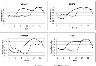
To examine the correlation between estimated wind energy output at Weatherford and electricity demand in Oklahoma, we obtained hourly electricity demand data for Oklahoma Gas and Electric (OGE) and Oklahoma Municipal Power Authority from FERC Form 714 [10]. While OGE and OMPA are not the only electric utilities in Oklahoma, data from other Oklahoma utilities was not available for our analysis. A complete data set of hourly electricity demand in Oklahoma is not vital for our analysis, since we are primarily concerned with the rela- tive variation in demand compared to wind and solar energy production.

We normalized both hourly wind production and hourly electricity demand for OGE and OMPA on a sea-

sonal basis; this normalized data is shown in Figure 3.

The annual correlation between wind production and

0 200 400 600 800 1000 1200 1400 1600

0 10 20 30 40 50 60

Po

we

r (

k

W)

Wind Speed (miles per hour)

Figure 1. Wind power curve for the GE 1.5SL turbine.

Figure 2. Variation in energy production (kWh, left axis) and percentage variation in production (volatility, right axis) for the simulated wind site in Weatherford.

2.2. Solar Production Modeling data, is 0.061. We note that unlike analyses of wind en-

ergy production and electricity consumption in other ar- eas of the US [3,11], there is a small but positive degree of correlation between our estimates of wind energy production in Weatherford and electricity consumption in portions of Oklahoma. We also observe more diurnal variability, on average, during the summer months than during other times of the year.

Five minute solar radiation data (W/m2) are utilized

along with TRNSYS, an energy simulation program, to

simulate photovoltaic energy production in Weatherford1.

e assume a flat-plate fixed-axis collector with tracking, W

0.4 0.5 0.6 0.7 0.8 0.9 1

1 5 9 13 17 21

N o rm a liz e d va lue Hours Winter 0.4 0.5 0.6 0.7 0.8 0.9 1

1 5 9 13 17 21

N o rm a liz e d va lue Hours Spring 0.4 0.5 0.6 0.7 0.8 0.9 1

1 5 9 13 17 21

N o rm alized value Hours Summer 0.4 0.5 0.6 0.7 0.8 0.9 1

1 5 9 13 17 21

N o rm alized va lu e Hours Fall

Demand Wind Produc on

Figure 3. Normalized average wind production at Weatherford and electricity demand in the OGE and OMPA service terri-tories.

and a conversion efficiency of 15%. A variety of factors affect the production of energy from photovoltaic mod- ules apart from the level of solar irradiance including dust and haze. We utilized detailed meteorological data from the ASOS station at Stafford Airport, a short dis- tance east of our measurement station for Weatherford to incorporate the impacts of dust on solar energy produc- tion. The simulated photovoltaic installation has an esti- mated capacity factor of 0.17.

We compared normalized photovoltaic energy produc- tion with normalized electricity demand and wind energy

production by season, as shown in Figure 4. We observe

the typical seasonal variations in photovoltaic production, with an extended period of peak photovoltaic production in the summer compared to other seasons. Graphically, we do not observe anti-correlation between wind and solar production of a particularly large magnitude; the seasonal correlations between wind and solar production for our case study are 0.27 in the wintertime, 0.2 in the spring, 0.21 in the summer and 0.21 in the fall.

2.3. Natural Gas Production Modeling

The natural gas turbine that we use in our analysis is a GE 10-1 combustion turbine with a nameplate capacity

of 10 MW and a combustion efficiency of 31.4%2 at the

time of this writing, the price of natural gas in Oklahoma was $6.96 per million BTU [12], implying a marginal energy cost of production of $75.63 per MWh. A heat rate curve for this specific turbine was not available, so we use the quadratic emissions model described in [13]

to estimate emissions of NOx and CO2 as a function of

the magnitude and speed with which production at the gas turbine is ramped up and down in response to fluc- tuations in solar and energy resource availability. While the method in [13] has been criticized [14], it seems ap-

propriate given the scale of our problem (i.e., power-

plant level operations).

2.4. Long Run Average Cost

The Levelized Cost of Electricity (LCOE, units of $/MWh) represents the long-run average cost of a power plant. We use the LCOE metric to compare the costs of a natural gas turbine with the costs of two coupled genera- tion installations. The first system couples output from a wind installation with the gas turbine, while the second couples output from wind and photovoltaic installations with the gas turbine. The LCOE measures the average

price required to break even over the long run—i.e., to

recover the present discounted value of all capital and operating costs. The LCOE is defined as [15]:

2_{Turbine performance data was obtained from}

http://www.gepower.com/businesses/ge_oilandgas/en/prod_serv/prod/g

as_turbine/en/ge10_1.htm. LCOE









rt

r FC e cf VC

0 0.2 0.4 0.6 0.8 1

1 5 9 13 17 21

No rm al iz e d   va lu e Hour Winter 0 0.2 0.4 0.6 0.8 1

1 5 9 13 17 21

No rm al iz e d   Va lu e Hour Spring 0 0.2 0.4 0.6 0.8 1

1 5 9 13 17 21

No rm al iz ed   Va lu e Hour Summer 0 0.2 0.4 0.6 0.8 1

1 5 9 13 17 21

No rm al iz e d   va lu e Hour Fall

Demand Wind Production Solar Production

Figure 4. Normalized average wind and solar energy production at Weatherford and electricity demand in the OGE and OMPA service territories.

where r is the annual discount rate; FC represents over-

night fixed costs, T is the relevant time horizon for the

project (assumed to be 20 years for all technologies), cf is

the project’s capacity factor, and VC is the variable cost

of producing a unit of energy. We assume that the over- night fixed costs are $500/kW for the natural gas plant [16], $2100/kW for the wind turbine [6] and $5000/kW for the photovoltaic installation [16].

3. Results

We simulate the operation of three systems producing a constant amount of power, and compare the cost and

emissions implications (CO2 and NOx) of each. The three

systems we consider in our analysis are a stand- alone gas combustion turbine; a coupled system of wind and natural gas; and a coupled system of wind, solar photo-voltaic and natural gas. In the latter two scenarios, the gas turbine is utilized for providing fill-in power as de-scribed in Section 1. The cost and emissions implica- tions are compared on a per-unit-energy basis, so we do not need to specify an explicit size for the system (al- though our capital cost figures in Section 2.4 implicitly assume utility-scale installations).

Given the capital and operating costs of the gas and wind turbines, and the high capacity factor of the mod-eled wind installation in Weatherford, the LCOE for the coupled wind/gas system is lower than for the gas system alone ($86.59/MWh for the coupled system versus $95.60/MWh for the natural gas turbine alone). The

LCOE of the coupled system is naturally sensitive to fluctuations in the fuel price for the gas turbine and the availability of the wind turbine; if the price of natural gas were to drop below $6/mmBTU then the gas turbine alone would be more economical. Because of the high capital costs of solar photovoltaic, and the low capacity factor, we find that coupling photovoltaics with the wind/gas system increases the LCOE to $223.24/MWh. Defining the integration cost for solar photovoltaics as the increase in (levelized) energy costs for each five- minute interval for the wind/solar/gas system versus the wind/gas system, we see that average integration costs for including photovoltaics in a portfolio of wind and fossil energy vary seasonally and range from between

$57/MWh to nearly $120/MWh (Figure 5).

Moreover, the emissions of NOx following the

integra-tion of photovoltaics into the wind/gas system increase

for the scenario that we simulated, although CO2

emis-sions from the coupled system decline. Figure 6(a)

shows that integrating wind and solar with the natural gas

turbine reduces CO2 emissions by 500 to 1000 tonnes per

month, assuming a system with 10 MW of renewables and 10 MW of natural gas turbine capacity. The incre-mental avoided emissions from coupling photovoltaics with the wind/gas system are relatively small, at 25

ton-nes per month. Figure 6(b) shows NOx emissions from

the three systems; coupling wind and solar with the

natural gas turbine increases NOx emissions by a factor

5 6 7 8 9 10 11 12

Av

e

ra

ge

En

e

rg

y

Cos

t

(ct

s/

kW

h

)

Figure 5. Average energy cost of integrating photovoltaics into the wind/gas portfolio.

950 1000 1050 1100 1150 1200 1250

CO

2

Em

issio

n

s

(i

n

to

n

n

es)

(a) CO2Emissions

0 1000 2000 3000 4000 5000 6000

NO

x

Em

issio

n

s

(k

g)

(b) NOxEmissions 

Gas Only Wind/Gas Wind/Solar/Gas

CO

2

NO

x

Figure 6. Emissions impacts from coupling wind and natural gas; and coupling wind, solar and natural gas. Panel (a) shows the decrease in CO2 emissions from coupling renewables and fossil fuels, while panel (b) shows the increase in NOx emissions.

4. Discussion and Conclusions

Our results on the emissions implications of coupling renewables and fossil fuels are consistent with previous research [13]. Coupling wind energy with a natural gas

turbine can potentially reduce long-run average produc- tion costs, although incrementally adding photovoltaics to the portfolio increases costs. We find that the coupled

wind/gas system has higher NOx emissions than simply

‐1000

‐500 0 500 1000 1500 2000 2500

Emi

ss

io

ns

Sa

vi

ngs

($

)

CO2 Emissions Savings Nox Emissions Costs Net Emissions Savings

CO2

NOx

Figure 7. Monetary savings, including emissions costs, from coupling wind and natural gas. We do not find any monetary savings from adding photovoltaics to the wind/gas capacity portfolio.

but lower CO2 emissions. Adding photovoltaics reduces

the CO2 emissions profile of the system slightly while

increasing the NOx profile.

In a scenario where emissions are priced, the reduction

in CO2 cost may outweigh the increase in NOx costs for

the wind/gas coupled system, yielding net savings (com-pared to running the gas-only system) depending on the

relative emissions prices. Using prevailing CO2 prices

from the European Market of $22.60 per tonne, and a

NOx price of $0.25/kg, we find that pricing emissions

leads to additional net savings for the wind/gas coupled

system (Figure 7). While there would be additional net

emissions cost savings from adding photovoltaics to the coupled system, the savings are not sufficient to offset the higher long-run average production cost.

The incentives for owners of renewable energy pro- jects to couple operations with controllable energy sources are still a matter of debate. In some territories that have adopted wholesale restructuring, such coupling would allow the owners to receive capacity payments. In territories where bilateral market activity is the dominant form of trade, coupled renewable and fossil projects may be able to sign “firm” energy contracts (subject to avail-ability of transmission), which typically sell at a pre-mium.

5. Acknowledgements

The authors would like to acknowledge support from the Wilson Endowment in the College of Earth and Mineral Sciences at Penn State for the purchase of Oklahoma Mesonet data; staff at the Oklahoma Mesonet project for assistance with the data; and Jeffrey Brownson and

Re-becca Hott for advice on modeling solar energy produc-tion.

REFERENCES

[1] NREL, “Wind Technologies Market Report,” 2010. www1.eere.energy.gov/wind/pdfs/51783.pdf

[2] US DOE, “20% Wind Energy by 2030: Transmission and Integration into the US Electric System,” 2008.

http://www.20percentwind.org/Final_DOE_Executive_Su mmary.pdf

[3] A. Fernandez, S. Blumsack and P. Reed, “Evaluating Wind-Following and Ecosystem Services for Hydroelec-tric Dams,” Center for Research in Regulated Industries Eastern Conference, Skytop, May 2011.

[4] E. Fertig and J. Apt, “Economics of Compressed Air En-ergy Storage to Integrate Wind Power: A Case Study in ERCOT,” Energy Policy, Vol. 39, No. 5, 2011. pp. 2330- 2342.doi:10.1016/j.enpol.2011.01.049

[5] E. Hittinger, J. Whitacre and J. Apt, “Compensating for Wind Variability Using Co-Located Natural Gas Genera- tion and Energy Storage,” Energy Systems, Vol. 1, No. 4, 2010, pp. 417-439.doi:10.1007/s12667-010-0017-2

[6] NREL, “Wind Energy Resource Atlas of the United States,” Renewable Resource Data Center (RReDC) Home Page, 2002.

http://rredc.nrel.gov/wind/pubs/atlas/appendix_A.html

[7] University of Oklahoma, Environmental Verification and Analysis Center.

http://www.ocgi.okstate.edu/owpi/Oksolarmap.gif

[8] Idaho National Laboratory, “Wind Turbine Power Curve Data,” 2012. http://www.inl.gov/wind/software/

[10] FERC, “Form 714-Pre-Electronic Filing Data: 1993- 2004,” Federal Energy Regulatory Commission, 2011. http://www.ferc.gov/docs-filing/forms/form-714/data.asp

[11] Carnegie Mellon Electricity Industry Center, “The Smart Grid: Sorting the Reality from the Hype,” 2009.

http://www.cmu.edu/electricity

[12] Price data from US Energy Information Administration, 2012.

http://www.eia.gov/dnav/ng/ng_pri_sum_dcu_nus_m.htm

[13] W. Katzenstein and J. Apt, “Air Emissions Due to Wind and Solar Power,” Environmental Science & Technology, Vol. 43, No. 2, 2009, pp. 253-258.

doi:10.1021/es801437t

[14] A. Mills, R. Wiser, M. Milligan and M. O’Malley, “Comment on ‘Air Emissions Due to Wind and Solar Power’,” Environmental Science and Technology, Vol. 43, No. 15, 2009, pp. 6106-6107.doi:10.1021/es900831b

[15] S. Stoft, “Power System Economics: Designing Markets for Electricity,” Piscataway, IEEE, 2002.