Point Transformations and Relationships among Linear Anomalous Diffusion, Normal Diffusion and the Central Limit Theorem

(1)

http://www.scirp.org/journal/am ISSN Online: 2152-7393

ISSN Print: 2152-7385

DOI: 10.4236/am.2018.92013 Feb. 28, 2018 178 Applied Mathematics

Point Transformations and Relationships

among Linear Anomalous Diffusion, Normal

Diffusion and the Central Limit Theorem

Donald Kouri

1,2*

, Nikhil Pandya

1,2

, Cameron L. Williams

2

, Bernhard G. Bodmann

2

, Jie Yao

3

1_{Department of Physics, University of Houston, Houston, Texas, USA} 2_{Department of Mathematics, University of Houston, Houston, Texas, USA}

3_{Department of Mechanical Engineering, Texas Tech University, Lubbock, Texas, USA}

Abstract

We present new connections among linear anomalous diffusion (AD), normal diffusion (ND) and the Central Limit Theorem (CLT). This is done by defin-ing a point transformation to a new position variable, which we postulate to be Cartesian, motivated by considerations from super-symmetric quantum mechanics. Canonically quantizing in the new position and momentum va-riables according to Dirac gives rise to generalized negative semi-definite and self-adjoint Laplacian operators. These lead to new generalized Fourier trans-formations and associated probability distributions, which are form invariant under the corresponding transform. The new Laplacians also lead us to gene-ralized diffusion equations, which imply a connection to the CLT. We show that the derived diffusion equations capture all of the Fractal and Non-Fractal Anomalous Diffusion equations of O’Shaughnessy and Procaccia. However, we also obtain new equations that cannot (so far as we can tell) be expressed as examples of the O’Shaughnessy and Procaccia equations. The results show, in part, that experimentally measuring the diffusion scaling law can determine the point transformation (for monomial point transformations). We also show that AD in the original, physical position is actually ND when viewed in terms of displacements in an appropriately transformed position variable. We illustrate the ideas both analytically and with a detailed computational exam-ple for a non-trivial choice of point transformation. Finally, we summarize our results.

Keywords

Generalized Fourier Analysis, Normal Diffusion, Anomalous Diffusion, Point Transformations, Canonical Quantization, Super Symmetric Quantum Mechanics

How to cite this paper: Kouri, D., Pandya, N., Williams, C.L., Bodmann, B.G. and Yao, J. (2018) Point Transformations and Relationships among Linear Anomalous Diffusion, Normal Diffusion and the Cen-tral Limit Theorem. Applied Mathematics, 9, 178-197.

https://doi.org/10.4236/am.2018.92013

Received: December 22, 2017 Accepted: February 25, 2018 Published: February 28, 2018

http://creativecommons.org/licenses/by/4.0/

(2)

DOI: 10.4236/am.2018.92013 179 Applied Mathematics

1. Introduction

The Central Limit Theorem (CLT) is closely related to the “normal diffusion” (ND) process and is relevant to many random processes [1][2][3][4][5]. The characteristic of ND is the fact that the mean square displacement (MSD) of a diffusing particle scales with time as 1

t . The CLT together with the assumed

zero mean and independence of increments implies that regardless of the mi-croscopic model, the transition probability at large scales is well approximated by a Gaussian [6]. When this Gaussian kernel is convolved with an initial proba-bility distribution, it evolves under time and after scaling tends to a Gaussian. We associate the evolution of the initial probability distribution in time with the semi-group generated by the Laplacian, 22

x

∂

∂ [7]. Because of the spectral

prop-erties of the standard Laplacian, the time dependent (Gaussian) solution is an “attractor” solution to the ND equation. However, in recent years, great interest has been focused on the phenomena of “anomalous diffusion” (AD) [5][8]-[35]. As can be seen from the above references, such processes are observed for a host of physical, chemical and biological phenomena. The AD processes of interest to us here are those for systems with an “effective position dependent diffusion coefficient”, resulting in time evolution governed by a generalized Laplacian (e.g., [4][5][15]). Herein, we provide the derivation of a general, infinite family of such Laplacians, including new ones not included in the landmark study of O’Shaughnessy and Procaccia [15]. In the case of AD, the characteristic feature is the fact that the MSD scales with time as 1

t β, where β is a real number. If

0.25≤ <

β

1, the process is termed “super diffusion” and if 1<

β

, the process is termed “sub-diffusion”. If 0< <

β

0.25 , the diffusion is termed ballistic. O’Shaughnessy and Procaccia were the first to show that many AD systems have exact, attractor solutions, called “stretched Gaussians”: 2

exp x ϑ 4Dt

ρ

_∝ _₋ + _

 

[15]. Here, D is a “constant effective diffusion coefficient”. We postulate the fact that these are computationally observed to be attractor solutions of the relevant differential equations implies that the standard CLT is “hidden” and applies also to AD associated with the diffusion equations we derive. In this paper, we show that this is indeed true.

The paper is organized as follows. In Section II, we summarize the solution of the ND equation, emphasizing its dependence on the Fourier transform (FT) of the probability function (the characteristic function) and noting that the charac-teristic function plays a key role in the proof of the CLT. In Section III, we dis-cuss important connections among super symmetric quantum mechanics (SUSY), Heisenberg’s uncertainty principle (HUP), point transformations (PT) (in order to deduce generalizations of the FT and the related Laplacians), and the CLT for diffusion in the new canonically conjugate “position”. In Section IV, we explore the relations among AD, ND, scaling laws and PT’s. In Section V, we provide a computational example for the point transformation,

( )

3

W x = +x x ,

(3)

DOI: 10.4236/am.2018.92013 180 Applied Mathematics diffusion equations and those in [15]. Finally, in Section VII, we summarize our results.

2. The Normal Diffusion Equation, Laplacian Semigroup and

the Central Limit Theorem

In the case of ND as a random process, the proof of the CLT is most readily based on the characteristic function, i.e., the FT of the probability distribution [24]. At its heart is the fact that the Gaussian is invariant under the FT. This is interesting because the ND equation is also exactly solved using the FT of the diffusion equation. This makes use of the fact that the Laplacian satisfies

2

2 2

d

e e

d

ikx ikx

k x

± _{= −} ± ₍₁₎

where eikx is the x-representation of the momentum eigenket, k2≥0 and e−ikx is the k-representation of the position eigenket. The FT kernel is therefore also an improper eigenstate of the standard Laplacian. This spectral relation en-sures that the Laplacian generates a semigroup. It results in the “directional” re-striction of solutions to the ND equation: the solution is stable only for increas-ing time. The semigroup does not possess a bounded inverse operator. It is also related to the attractor character of the solution to the ND equation [7]. The Gaussian minimizes the HUP for position and momentum and this provides a rigorous basis for the FT [36][37]. The diffusion equation,

( )

x t, D 22

( )

x t, ,

tρ x ρ

∂ ₌ ∂

∂ ∂ (2)

where D is constant, becomes

( )

2

( )

ˆ k t, k Dˆ k t, ,

tρ ρ

∂

= −

∂ (3)

under the FT ˆ

( )

1 _{d exp}

(

) ( )

2π

f k ∞ x ikx f x

−∞

 

= −

 



∫

. This is easily integrated (in time), yielding

( )

(

2

)

( )

ˆ k t, exp Dk t ˆ k, 0 .

ρ

= −

ρ

(4)

The inverse FT of a product of functions of k yields the exact convolution so-lution

( )

[

]

1 2

(

)

2

(

)

, 4π d exp 4 , 0 .

x t Dt x x x Dt x

ρ − ∞ ρ

−∞ ′  ′  ′

=

_∫

_− − _ (5)

Clearly, if ρˆ

( )

k, 0 is equal to 1, ρ

(

x′, 0

)

=δ

(

x′−x₀

)

(the diffusing particle

is localized initially at x=x0, with time dependence given by

( )

(

)

2

0

, exp 4

x t C x x Dt

ρ ₌ _{− −} 

 ). For any initial probability distribution whose

FT is differentiable, the long-time behavior will be dominated by the overall Gaussian envelope

(

2

)

exp −x 4Dt (simply expand the square in the exponent

in Equation (5) and factor out

(

2

)

exp −x 4Dt ). The 1 2

t− in the normalization

(4)

DOI: 10.4236/am.2018.92013 181 Applied Mathematics the measure dx. Then the MSD varies as 2Dt (note, the slope of the MSD is

not necessarily equal to one). We thus observe the role of the CLT as implying that the time dependence of any initial distribution, evolving according to Equa-tion (2), will tend to a Gaussian distribuEqua-tion envelope after a sufficiently long time. We stress that the characteristic function proof of the CLT also rests on the facts that the Gaussian is invariant under the FT and the FT satisfies the convo-lution theorem. These properties are related to the semigroup structure of the standard Laplacian.

3. Super Symmetric Quantum Mechanics, Heisenberg’s

Uncertainty Principle, Point Transformations, Canonical

Quantization, Generalized Fourier Transforms and

Laplacians

Recently, we have explored connections among super symmetric quantum me-chanics (SUSY), Heisenberg’s uncertainty principle (HUP), point transforma-tions (PT) and generalized Fourier transforms (GFT) [36][37][38]. We briefly summarize the relevant details here. A mathematically rigorous derivation of the FT (and its generalization) from the HUP has recently been given [36][37]. The fundamental starting point is that the minimum uncertainty state, ψmin , satis-fies

min

ˆ

min

ˆ

.

x

ψ

= −

ik

ψ

(6)

The state ψmin cannot be an eigenstate simultaneously of both the position and momentum operators since they do not commute (_{x k}_ˆ,ˆ =_i₁ˆ

  ). Explicitly, we note that Equation (6) reminds one of the property of simultaneous eigen-vectors of commuting operator observables, _{A B}ˆ ˆ_, _:

ˆ _, _, _,

A a b =a a b (7)

ˆ _, _, _,

B a b =b a b (8)

ˆ _, a ˆ _, _.

A a b B a b b

⇒ = ₍₉₎

The uncertainty product for such operators as _{A B}ˆ ˆ_, _{has course}_,_{the absolute}

minimum value of zero and the simultaneous eigenvector is the only vector ap-pearing in the above equations. The fact that the uncertainty product for posi-tion and momentum is positive definite results from the fact that neither

min

ˆ

xψ nor −ikˆ

ψ

_min can be simply proportional to the state ψ_min . The

(5)

DOI: 10.4236/am.2018.92013 182 Applied Mathematics The 1-D SUSY formalism is built on a program to make all systems (on the domain −∞ < x < ∞) look as much as possible like the harmonic oscillator, whose ground state also satisfies Equation (6). In the ladder operator notation, this equation is

min min min 0

1 _ˆ

ˆ ˆ 0

2 x ik ψ aHO ψ ψ ψ

 +  = = ⇒ =

  (10)

In the coordinate representation, aˆ_HO is

(

x+d dx

)

2 . In 1-D SUSY, the ground state is restricted to the form

( )

0 0 0 exp ₀d

x

x x W x

ψ

=

ψ

__−

_∫

′ ′ __₍₁₁₎

for W’s such that the ground state is 2

L . Choosing the zero of energy to be that

of the ground state, one finds that the potential of the system is given by

2 d 2 , d

W

V W

x

 

=_ − _

  (12)

and in terms of the position representation, the ground state satisfies

( )

0 0

1

ˆ

d d 0.

2W x + xψ =aWψ = (13) As noted previously, this immediately implies that the ground state, ψ0, mi-nimizes the uncertainty product ∆ ∆W k (=1) and suggests that one ought to be able to obtain a new transform under which ψ0 will be form invariant [36]

[37][41]. Unfortunately, since the commutator of W and d dx is proportional

to dW dx, which is constant only for W = x + constant, the desired transform

kernel cannot be the simple FT kernel. As a consequence, we do not actually use the SUSY expressions directly to derive the desired transform. We remark that in the SUSY community, W is interpreted as a “super potential”, based on Equa-tion (9). In our approach, we shall interpret W to be a generalized “posiEqua-tion” va-riable, based the facts that: 1) ψ0 minimizes ∆ ∆W k and 2) the quintessential choice of W is that for the harmonic oscillator, where W is precisely the par-ticle’s “generalized position” [36][40][41][42][43].

Recently, in [37], we explored choosing W to represent a point transformation of the usual position, such that 1) the domain of W is −∞ <W< ∞, (extension

to the half line can be done) 2) the domain of the canonically conjugate mo-mentum is also −∞ <PW< ∞, 3) the transformation is invertible and 4) both W and PW can be interpreted as Cartesian-like coordinates. One expression that satisfies the above is the polynomial [37]

( )

2 1 1

, J

j j j

W x a x

+

=

∑

₍₁₄₎

(6)

DOI: 10.4236/am.2018.92013 183 Applied Mathematics Assuming that W(x) satisfies the above conditions [37], the classical canoni-cally conjugate momentum, PW, is required to satisfy

{

W P, _W

}

=1, (15)

where

{ }

, is the Poisson bracket with respect to the original Cartesian-like

position and momentum [37][38]. It is easily shown that the classical canonical momentum can be expressed in the form

( )

1

1 1

.

d d

W x

P p g x

W W

x x

α α

−

= +

   

   

   

(16)

Invoking Occam’s razor, we set the integration constant along a constant-x integration path, g(x), equal to zero. Since PW above satisfies Equation (15) for all α, we then apply Dirac’s canonical quantization to obtain the generalized po-sition and momentum operators (in the W-representation). This quantization consists of replacing the observables by operators, the Poisson bracket by the commutator of the operators and the scalar 1 by i times the identity operator

[38]:

ˆ ˆ ˆ_, _1, _1,

W

W P i

  = =

   (17)

ˆ _,

W=W (18)

d ˆ _.

d

W

P i

W

= − (19)

We stress that these operators are manifestly self adjoint in the W-representation, with the measure dW. In addition, the minimizer of ∆ ∆W PW is obviously the Gaussian,

(

2

)

exp −W 2 , since

min min

d . d

W

ψ

ψ = − (20)

As in the case of the original position and momentum operators, ψmin is in-variant under the “W-Fourier transform (W-FT) kernel”:

(

)

(

)

exp 2π , exp 2π ,

W K = iKW K W = −iKW (21)

, .

W K

−∞ < < ∞ − ∞ < < ∞ (22) This is analogous to the FT in terms of x and k. This transform satisfies the convolution theorem under the measure dW or dK. We note that in the W-representation, since ˆ

W

P is self adjoint, we have the four equivalent, exact

expressions:

2

2 d

ˆ ˆ ˆ ˆ ˆ ˆ ˆ ˆ _,

d

W W W W W W W W

P P P P P P P P

W

+ + + +

− = − = − = − = (23)

ˆ _{ˆ ,}

W W

P =P+ (24)

which are all obviously self adjoint under the measure dW. The above relations are at the heart of our approach. The transformation that preserves the W-Gaussian

(

)

(

2

)

(7)

(

)

(

)

2 2 2 d

exp exp .

dW ±iKW = −K ±iKW (25)

Again, the W-Laplacian possesses a negative semi-definite spectrum so it is evident that this transform kernel possesses all the properties of the FT, includ-ing the fact that it supports a semigroup property.

We also note that there exists a generalized W-harmonic oscillator, with ground state satisfying [36][37]

(

2

)

0

1 d d

ˆ ˆ exp 2 0.

2 d d

W W

a a W W W

W W

ψ

+ ₌ ₋ ₊  ₊  ₋ ₌

  

   (26)

The diffusion equation describing independent random motion in W is ob-viously 2 2, D t W ρ ρ ∂ ₌ ∂

∂ ∂ (27)

where here, D is a constant diffusion coefficient. It follows that the exact solution of Equation (27) is obtained using the W-FT kernel Equation (21), yielding

(

)

(

)

2

(

)

, d exp 4 , 0 ,

W t W W W Dt W

ρ =

_∫

_−∞∞ ′ _− − ′ _ρ ′ (28)

where ρ

(

W′, 0

)

is any proper, initial distribution.

The “characteristic function” underlying the above expression is

( )

(

2

)

(

)

ˆ

K t

,

exp

DK t

ˆ

K

, 0 .

ρ

=

−

ρ

₍₂₉₎

If ρ

(

W′, 0

)

=δ

(

W′−W0

)

, then ρˆ

(

K, 0

)

equals one and the distribution is a Gaussian centered at W0. Note that in general, ρ

(

W t,

)

involves a positive function of time times a Gaussian envelope, 2

exp



_

−

W

4 Dt



_

. The analysis of the CLT for probability distributions in W is identical to that for the normal probability distribution [24].

We next consider the situation where we quantize Equations (23)-(24) in the x-representation (we do not invoke the chain rule). Because of the ambiguity of operator ordering, we consider the following explicit expressions for a genera-lized momentum operator and its adjoint, involving the parameter α:

1 d 1 ˆ _, d d d d d W i P x W W x x α α − − =             (30) 1 d 1 ˆ _. d d d d d W i P x W W x x α α + − − =             (31)

But these operators are obviously not self adjoint under the measure dx ( ex-cept in the case where α = 1/2)! Normally, they are discarded and replaced by their arithmetic average.

(8)

transfor-DOI: 10.4236/am.2018.92013 185 Applied Mathematics mation. Thus, Equation (30) is self adjoint under the measure

(

)

1 2

dx dW dx −α

and Equation (31) is self adjoint under the measure

(

)

2 1

dx dW dx α− . When

al-pha equals 1/2, the measure for self adjointness reduces to simply dx.

We remark that, as shown above in Equation (23), in the W-domain, all four Laplacians possess the W-Gaussian as the ground state solution of the W-HO. Also, all four Laplacians satisfy Equation (25) in the W-domain. Thus, all four Laplacians are not only self adjoint in the x-representation but they also are all negative semi-definite operators which have an underlying semigroup structure regardless of their explicit form in the x-domain. Each of the four Laplacians will be self adjoint in the x-domain but only with appropriate measures. We now ex-plicitly explore the forms of these Laplacians in the x-domain. It is convenient to group them in two pairs of two. This is because the forms

(

)

(

)

(

)

1 2 2

1 d 1 d 1 ˆ ˆ

d d

d d d

W W

P P

x x

W xα W x α W x α

+

−

∆ = − =

∂ ∂ ∂ (32)

and

(

)

(

)

(

)

2 1 2 1

1 d 1 d 1 ˆ ˆ

d d

d d d

W W

P P

x x

W x α W x α W x α

+

− −

∆ = − =

∂ ∂ ∂ (33)

are already manifestly self adjoint under the measure dx. The other pair is

(

)

(

) (

)

3 1

1 d 1 d 1 ˆ ˆ

d d d d

W W

P P

x W x x

W x −α W xα

∆ = − = (34)

and

(

)

(

) (

)

4 1

1 d 1 d 1 . d d d d

d d d d

W W

P P

x W x x

W xα W x α

+ +

−

∆ = − = (35)

The above two Laplacians, ˆ ˆ

W W

P P+ +

− and ˆ ˆ

W W

P P

− , require different measures from one another as well as from the first two Laplacians (except for α =1 2). We stress that both are self adjoint operators in the x-domain, with the correct measure for ∆3 being

(

)

1 2

dx dW dx −α and the correct measure for ∆4 being

(

)

2 1

dx dW dx α− . We next note that all four of these Laplacians support HO-like

Hamiltonians. We define

(

)

(

)

(

)

(

)

1 1 1

1 1 d 1 1 d 1

ˆ

2 d d d d d d d d d d

H W W

x x

W xα W x −α W x −α W x α

  

  

= − − +

  

   (36)

(

)

(

)

(

)

(

)

2 1 1

1 1 d 1 1 d 1

ˆ

H W W

x x

W x −α W xα W x α W x −α

  

  

= _− + _ + _

   (37)

(

)

(

)

(

)

(

)

3 1 1

1 1 d 1 1 d 1

ˆ

H W W

x x

W x −α W x α W x −α W xα

  

  

= − + +

  

   (38)

(

)

(

)

(

)

(

)

4 1 1

1 1 d 1 1 d 1

ˆ

H W W

x x

W x α W x −α W x α W x −α

  

  

= _− + _ + _

   (39)

(9)

DOI: 10.4236/am.2018.92013 186 Applied Mathematics 3 and 4. It is easily seen that Hamiltonians 1 and 3 will have identical ground states, satisfying

(

)

1

(

)

(

)

(

2

)

1 d 1

d d exp 2 0. d

d d d d

W W x W

x

W x W x

α α α −   + − =    

  (40)

Hamiltonians 2 and 4 will also have identical ground states, satisfying

(

)

(

)

(

)

(

)

1 2

1

1 d 1

d d exp 2 0. d

d d d d

W W x W

x

W x W x

α α α − −   + − =    

  (41)

These follow from the fact that the ground states are annihilated by the right hand operator in the respective factored Hamiltonians. We stress that, in the general case, none are simple Gaussians. Rather, the influence of the point transformation is clearly evident. Of course, if one sets

α

=0 or 1, then we see that the “stretched Gaussian” is one of the ground states. However, there is a second (bi-orthogonal partner) ground state which, in general, will be a mul-ti-modal distribution. Because of the monotonic increasing character of the PT,

dW dx is never negative and the ground state is always positive semi-definite.

This is new and it reflects the fact that our formalism is closely related to the “Coupled SUSY” formalism introduced elsewhere [42][43].

The next question of importance is: What are the eigenstates of the four x-domain Laplacians? These will provide the transformations under which the various generalized HO ground states are invariant (in analogy to the FT and the Gaussian distribution). Of course, in the “W-world”, there is only the W-FT, re-sulting from the W-Laplacian, having only the simple W-Gaussian as the solu-tion of the diffusion and HO equasolu-tions. We begin by considering the first two Laplacians. In this case, the explicit, analytical transforms have been derived in [36]for monomial W’s and α = 0. In that case, the first equation is

(

)

2 2

d d 1 ˆ ˆ

d d d d

K

W W K K

P P K

x W x x

+ Φ

− Φ = = − Φ ₍₄₂₎

where 2 0

K ≥ (the Laplacian is negative semi-definite and self adjoint under

the measure dx). The unitary transformation was derived restricting W to the monomial form

W x

( )

=

x

β. The result is

( )

[ ]

( )

1 2

1 1 2 1 1 2

1

sgn 2

K kx J kx i kx J kx

β

β β β

β β

−

− + −

 

Φ = _ − _

  (43)

which is unitary under the measure dx. The stretched Gaussian,

(

2

)

exp − x β 2

is invariant under this transform. The second transform equation is

(

)

(

)

2

2 2

1 d 1

dW dx dx dW dx Φ = − ΦK K K (44)

and the unitary transform (under the measure dx), ΦK, is given by

( )

1 ( 1 2)

( )

_{( )}

( 1 2)

( )

1 2 1 2

1

sgn sgn

2

K J i J

β β β β

β β

η − η − η η η − η

−

 

Φ = _ + _

 

 ₍₄₅₎

(10)

DOI: 10.4236/am.2018.92013 187 Applied Mathematics In this case, it is the, in general, multi-modal distribution

(

)

(

2

)

dW dx exp −W 2 which is invariant.

The transformations for the second two Laplacians are easily obtained for general values of α. For the Laplacian ∆3, the result is

(

)

(

)

2

3 K

K

,

K

d

W

d

x

exp

iKW

2π .

α

ϕ

ϕ ϕ

∆

= −

=

±

₍₄₆₎

The result for the Laplacian ∆4 is given by

(

)

1

(

)

2

4 K K K, K dW dx exp iKW 2π .

α

ϕ

ϕ ϕ

−

∆  = −   = ± (47)

It is easily seen that these are bi-orthogonally related, since

3 4

+

∆ = ∆ (48)

and that (in Dirac notation),

(

)

,

K K K K K K

ϕ ϕ ′ = ϕ ϕ ′ =δ − ′ (49)

ˆ1 dK ϕK ϕK dK ϕK ϕK .

∞ ∞

′ ′

−∞ −∞

=

_∫

 =

_∫

 (50)

Thus, the bi-orthogonal transforms serve to carry out Fourier-like transfor-mations of the ground states of the GHOs. The ground state solution,

(

)

(

2

)

dW dx αexp −W 2 , when transformed using ϕK under the measure dx, will produce the stretched Gaussian. The same is true when

(

)

1

(

2

)

dW dx −αexp −W 2 is transformed by ϕK under the measure dx. This explicitly shows how the underlying CLT for the W-domain Laplacian and W-Gaussian will be manifested in the x-representation.

4. Anomalous Diffusion and Normal Diffusion

We now discuss the implications of the above for diffusion. We consider the four linear diffusion equations

, 1 - 4.

j

j j

D j

t

ρ

ρ ∂

= ∆ =

∂ (51)

In the cases j=1, 2, the Laplacians are self adjoint under dx. When we choose monomial W’s with

α

=0 and j=1, transformation under Φ_K leads to

2 1

1

ˆ

ˆ .

DK t

ρ _ρ

∂ = −

∂ (52) When we choose the same alpha and j = 2, transformation under ΦK again

yields

2 2

2

ˆ

ˆ .

DK t

ρ _ρ

∂ _{= −}

(11)

same as that resulting from the inverses of Φ Φ_K,_K). This transformation

pos-sesses a convolution theorem and in the W-domain, all behave in time like nor-mal diffusion! We conclude that all of the linear diffusion equations derived herein are subject to the CLT associated with Gaussian distributions. The above analysis holds in general for any proper choice of PT but the above analysis for the j = 1, 2 cases has only been explicitly realized for the monomial case with al-pha equal to zero. In the case of j = 3, 4, everything applies for general point PT’s, including polynomials [37].

For simplicity, we shall illustrate these ideas using the specific example of the j = 3 case for alpha equal to zero. The transform equation is then

( )

(

)

2

(

( )

)

1 d 1 d

exp exp .

dW d dx x dW d dx x iKW x K iKW x

    _± _{= −} _±

   

    (54)

The diffusion equation is

d 1 d 1 d

.

dt D W x x W x x

ρ

   

_ρ

= _∂ _{∂ ∂}  _∂ _{∂ ∂} 

    (55)

The corresponding x-domain GFT kernel from Equation (21) is given by

( )

1

(

( ) ( )

)

exp .

2π

K W iW k W x

ϕ = ± (56)

When applied in the form Equation (56), the measure is d d d

W x

x . We note

that requiring K to have the same functional dependence on k as W(x) on x en-sures the argument of the exponential is dimensionless and that the measure for integration over K in the k-domain is d d d

( )

d

W k

K k

k

= . After applying the GFT

and using Equation (25), the exact solution (in the k-domain) is

( )

(

)

(

( )

2

)

(

( )

)

ˆ W K ,t exp W k Dt ˆ W K , 0 .

ρ = − ρ ₍₅₇₎

The inverse GFT (which satisfies the convolution theorem in the variable W) then leads to the probability distribution at time t:

( )

(

)

( )

(

( )

2

)

(

( )

)

, d exp 4 , 0 .

W x t W x W x W x Dt W x

ρ

=

_∫

′ −_ − ′ _

ρ

′ (58)

We stress that as derived, this is a probability distribution in the variable W(x), not the variable x. The measure for normalization will be

d

(

W x

( )

)

, the normalization constant will be

[

]

1 2

4 π

Dt

− and the MSD will be proportional to 1

t . The diffusion is normal in the variable W.

However, Equation (58) can also be interpreted as a probability distribution in the variable x. It is a positive definite function of x and can be normalized to 1 under the measure dx:

( )

(

)

dxρ W x , 0 1.

∞

−∞ =

(12)

DOI: 10.4236/am.2018.92013 189 Applied Mathematics If, e.g., W x

( )

=xβ , the integration will be transformed to the variable

1 2

x→x t β and the normalization will be proportional to t−1 2β. The average

value of x will be zero (for symmetric initial distributions) and the MSD will scale as

1

MSD∝t β. (60) This is, of course, the scaling for AD: the probability distribution is inter-preted as applying to the physical position variable, x, rather than to the canoni-cal variable, W x

( )

=xβ. The range 0.25< <

β

1 corresponds to super d iffu-sion, the range 0< <

β

0.25 corresponds to ballistic diffusion and

β

>1 cor-responds to sub-diffusion. However, because the Laplacian satisfies Equation (25), the time evolution will still be such that the CLT is satisfied. The normali-zation has nothing to do with the fact that the time evolution is governed by the attractor, whether we express it in the W- or the x-domain. Similar scaling re-sults apply in the general cases.

5. A Computational Example for the Polynomial

( )

3

W x

= +

x

We illustrate our results by the numerical example of a polynomial choice of PT:

( )

3

.

W x = +x x (61)

We assume the initial distribution to be

(

)

(

2

)

, 0

exp

1000

.

W

ρ

=

−

₍₆₂₎

This is very localized at W = 0, implying that it is centered at x = 0. The diffu-sion equation expressed in the x-domain is given by

2 2

1 1 . 1 3 1 3

D

t x x x x

ρ ρ

∂ ₌ ∂ ∂

∂ + ∂ + ∂ (63)

We note that in the region x 1, W is, to a very good approximation, equal

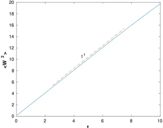
to x but as the particle diffuses to larger magnitude values of x, it quickly transi-tions to being dominated by the cubic x-dependence. The W-domain results are shown in Figure 1 and Figure 2, where it is obvious that the diffusion is normal, since Equation (63) becomes Equation (27).

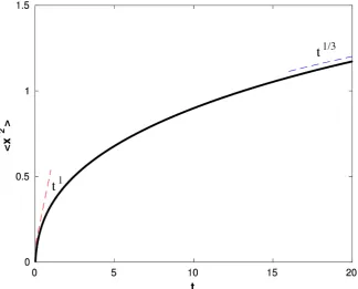
Of greater interest are the results where we interpret our density in the x-domain and use the Laplacian resulting in the diffusion Equation (63). The results are displayed in Figure 3 and Figure 4.

It is clear that at the earliest time, the linear x-dependence dominates the Lap-lacian and the diffusion is essentially normal, with the normal MSD t-scaling becoming more and more accurate as t approaches zero. At longer times, the cu-bic x-dependence dominates the Laplacian and we see that the MSD behavior tends to that of 1 3

t , just as one expects. While for more complicated polynomial

(13)

[image:13.595.212.537.70.331.2]

Figure 1. Time evolution in W coordinate is normal. The different color graphs corres-pond to times of diffusion, as indicated in the inset.

Figure 2. MSD in W coordinate. Diffusion is normal. The solid line is the result of solv-ing the W-domain diffusion equation. The dashed line is the curve resultsolv-ing from the MSD scaling as the time, t.

[image:13.595.208.536.377.634.2]

(14)

[image:14.595.211.535.66.324.2]

Figure 3. Evolution in x coordinate is anomalous. The different color graphs correspond to times of diffusion, as indicated in the inset.

Figure 4. Short and long time behavior of MSD in x. The early time shows ND and the later time AD. The red dashed curve beginning at t = 0 is the linear in time scaling law and the dashed blue curve at large time is the 1/3 power of t scaling law.

[image:14.595.211.536.373.634.2]

(15)

6. Relationship between Our Diffusion Equations and the

O’Shaughnessy-Procaccia Equations

As formulated, our analysis and diffusion equations are very general and appli-cable both to fractal and non-fractal AD processes. Furthermore, for specific choices of our parameters, our equations exactly incorporate the radial diffusion equations of [15]. This might appear somewhat strange since our equations are defined on the entire real line while those of O’Shaughnessy and Procaccia are for radial variables on the half line. In fact, it is only a subset of our equations that incorporate the O’Shaughnessy and Procaccia equations [36]. The Lapla-cians are, explicitly, Equation (32) for α = zero. They were first derived on the half line and then extended to the full real axis and these are the particular equa-tions that capture those of reference [15]. We explicitly prove this below. The equations of interest are given by

1 1

1

.

c c

D x

t x x x

ϑ

ρ − − ρ

−

∂ ∂ ∂

=

∂ ∂ ∂ (64) To transform this to our form of equations, we define the auxilliary variable

,

c

y=x (65)

in the equation above. It easily follows that

1 2 2 2

1 .

c c

c

D

x c D x

x x y y

x

ϑ ϑ

− − − −

−

∂ ∂ ∂ ∂

=

∂ ∂ ∂ ∂ (66)

Here, c is the dimension (non-integer c’s correspond to fractal cases). If one next defines the parameter

2 c 2,

β ϑ= − + ₍₆₇₎

then Equation (66) becomes

(

)

2 2 2 2 2 2

2 2 2

1 1

,

c

c D x c D c D

y y y y y y W y y

ϑ

β β

− −

−

∂ ∂ ∂ ∂ ∂ ∂

= =

∂ ∂ ∂ ∂ ∂ ∂ ∂ ∂ (68)

where

( )

, c.

W y =yβ yβ =xβ (69)

The parameters, c,ϑ remain independent of one another. Of course, this is

exactly our diffusion equation for the Laplacian in Equation (32) with

α

=0. (In addition, we note that Equation (33) also captures the O’Shaughnessy and Procaccia equations for the specific value

α

=1.) It is important to note, how-ever, that even for the simplest monomial cases, with α≠0,1, all four of our

Laplacians in Equations (32)-(35)differ from those of reference [15]. These new diffusion equations are also currently under computational study in our group.

7. Conclusions

(16)

DOI: 10.4236/am.2018.92013 193 Applied Mathematics using the relevant generalized coordinate. AD as a function of x is simply “dis-guised ND” in W.

Second, we have shown that when linear anomalous diffusion is analyzed in terms of the appropriate PT displacement variable, the usual CLT applies. Of course, this in no way alters the fact that the situation is much more complex in the case of nonlinear diffusion [4][5][6].

Third, our results show that, for such AD systems, experimental d etermina-tion of the anomalous scaling leads directly to the identification of the relevant generalized coordinate, W(x) (in the case of the monomial choice of W(x)). Certainly, for the example case of

( )

3

W x = +x x , it is also quite easy to extract

the relevant PT from the numerical data. For more general polynomial PTs, it will, naturally, be more complicated but the experimental scaling should still give information as to the relevant PT and effective displacement variable.

Fourth, we recall that the CLT is related to approximating the semigroup gen-erated by the Laplacian operator. Because of this, we expect that any diffusion process for which a “proper” Laplacian operator exists will have an attractor so-lution that is invariant under the generalized transform and is an eigenfunction of the corresponding HO. It will be of interest to explore treatment of Levy processes using fractional powers of the generalized Laplacians.

Fifth, we have obtained linear diffusion equations that not only capture all those of reference [15], but include infinite families of new equations for the values 0< <

α

1. It will be of interest to explore whether any experimental data correspond to these new linear diffusion equations.

Sixth, in our analysis, we considereddiffusion in a 1D“Cartesian system” with a constant diffusion coefficient,D. It readily generalizes to any number of Carte-sian random variables by simply summing the generalized Laplacians for each degree of freedom. We also point out that the scaling need not be the same in each degree of freedom. This will be important for anisotropic diffusion processes. It is also possible to introduce non-Cartesian coordinates (e.g., in a 3-D Cartesian

ˆ

ˆ ˆ

x iβ y jβ z kβ

= + +

W system, one can define 2

r β =W W⋅ , along with angular variables to obtain a “spherically symmetric diffusion operator”). As in quantum mechanics, these should be derived by a coordinate transformation of the Carte-sian-like Laplacians.

Finally, we are currently exploring the more general and difficult case of non-linear diffusion equations using our generalized Fourier transform me-thods.

Acknowledgements

(17)

References

[1] Gillespie, D.T. and Seitaridou, E. (2013) Simple Brownian Motion. Oxford Univer-sity Press, Cambridge, U.K.

[2] Feller, W. (1971) An Introduction to Probability Theory and Its Applications. Vol. 2, Wiley, New York.

[3] Harrison, J.M. (1971) Brownian Motion and Stochastic Flow Systems. Wiley, New York.

[4] Tsallis, C. (2005) Nonextensive Statistical Mechanics, Anomalous Diffusion and Central Limit Theorems. Milan Journal of Mathematics, 73, 145-176.

https://doi.org/10.1007/s00032-005-0041-1

[5] Plastino, A. and Rocca, M.C. (2011) Inversion of Tsallis’ q-Fourier Transform and the Complex Plane Generalization. arXiv:1112.1985v1 [math-phys]

[6] Einstein, A. (1905) Uber die von der molecular kinetischen Theorie der Wärmege-forderte Bewegung von in ruhenden Flüssigkeitensuspendierten Teilchen. Ann. der Phys., 17, 549. https://doi.org/10.1002/andp.19053220806

[7] Goldstein, J. (1985) Semigroups of Linear Operators and Applications. Oxford University Press, New York.

[8] Tsallis, C. (2009) Introduction to Nonextensive Statistical Mechanics. Springer, New York.

[9] Metzler, R. and Klafter, J. (2000) The Random Walk’s Guide to Anomalous Diffu-sion: A Fractional Dynamics Approach. Physics Reports, 339, 1-77.

https://doi.org/10.1016/S0370-1573(00)00070-3

[10] Metzler, R. and Klafter, J. (2004) The Restaurant at the End of the Random Walk: Recent Developments in the Description of Anomalous Transport by Fractional Dynamics. Journal of Physics A: Mathematical and General, 37, R161-R208.

https://doi.org/10.1088/0305-4470/37/31/R01

[11] Metzler, R., Jeon, J.H., Cherstvy, A.G. and Barkai, E. (2014) Anomalous Diffusion Models and Their Properties: Non-Stationarity, Non-Ergodicity, and Ageing at the Centenary of Single Particle Tracking. Physical Chemistry Chemical Physics, 16, 24128-24164.https://doi.org/10.1039/C4CP03465A

[12] Ben-Avraham, D. and Havlin, S. (2000) Diffusion and Reactions in Fractals and Disordered Systems. Cambridge University Press, London.

https://doi.org/10.1017/CBO9780511605826

[13] Sornette, D. (2001) Critical Phenomena in Natural Sciences. Series in Synergetics, Springer, New York.

[14] Risken, H. (1984) The Fokker-Planck Equation. Springer, New York, 63-95.

https://doi.org/10.1007/978-3-642-96807-5_4

[15] O’Shaughnessy, B. and Procaccia, I. (1985) Analytical Solutions for Diffusion on Fractal Objects. Physical Review Letters, 54, 455-458.

https://doi.org/10.1103/PhysRevLett.54.455

[16] Plerou, V., Gopikrishnan, P., Nunes Amaral, L.A., Gabaix, X. and Stanley, H.E. (2000) Economic Fluctuations and Anomalous Diffusion. Physical Review E, 62, R3023-R3026.

[17] Barkai, E., Aghion, E. and Kessler, D.A. (2014) From the Area under the Bessel Ex-cursion to Anomalous Diffusion of Cold Atoms. Physical Review X, 4, Article ID: 021036.https://doi.org/10.1103/PhysRevX.4.021036

(18)

Diffu-DOI: 10.4236/am.2018.92013 195 Applied Mathematics sion. Physical Review A, 45, 833-837.https://doi.org/10.1103/PhysRevA.45.833

[19] Kärger, J., Pfeifer, H. and Vojta, G. (1988) Time Correlation during Anomalous Diffusion in Fractal Systems and Signal Attenuation in NMR Field-Gradient Spec-troscopy. Physical Review A, 37, 4514-4517.

https://doi.org/10.1103/PhysRevA.37.4514

[20] Grebenkov, D.S. (2007) NMR Survey of Reflected Brownian Motion. Reviews of Modern Physics, 79, 1077-1137. https://doi.org/10.1103/RevModPhys.79.1077

[21] Gefen, Y., Aharony, A. and Alexander, S. (1983) Anomalous Diffusion on Percolat-ing Clusters. Physical Review Letters, 50, 77-80.

[22] Zanette, D.H. and Alemany, P.A. (1995) Thermodynamics of Anomalous Diffusion. Physical Review Letters, 75, 366. https://doi.org/10.1103/PhysRevLett.75.366

[23] Bohr, T. and Pikovsky, A. (1993) Anomalous Diffusion in the Kuramoto-Sivashinsky Equation. Physical Review Letters, 70, 2892-2895.

[24] Kleuke, A. (2014) Probability Theory. Springer, New York.

[25] Klafter, J. and Sokolov, I.M. (2005) Anomalous Diffusion Spreads Its Wings. Phys-ics World, 18, 29-32. https://doi.org/10.1088/2058-7058/18/8/33

[26] Sancho, J.M., Lacastra, A.M., Lindenberg, K., Sokolov, I.M. and Romero, A.H. (2004) Diffusion on a Solid Surface: Anomalous Is Normal. Physical Review Letters, 92, Article ID: 250601.https://doi.org/10.1103/PhysRevLett.92.250601

[27] Lapas, L.C., Morgado, R., Vainstein, M.H., Rubi, J.M. and Oliveira, F.A. (2008) Khinchin Theorem and Anomalous Diffusion. Physical Review Letters, 101, Article ID: 230602.https://doi.org/10.1103/PhysRevLett.101.230602

[28] Liu, B. and Goree, J. (2008) Superdiffusion and Non-Gaussian Statistics in a Dri-ven-Dissipative 2D Dusty Plasma. Physical Review Letters, 100, Article ID: 055003.

[29] He, Y., Burov, S., Metzler, R. and Barkai, E. (2008) Random Time-Scale Invariant Diffusion and Transport Coefficients. Physical Review Letters, 101, Article ID: 058101.https://doi.org/10.1103/PhysRevLett.101.058101

[30] Amir, A., Oreg, Y. and Imry, Y. (2010) Localization, Anomalous Diffusion, and Slow Relaxations: A Random Distance Matrix Approach. Physical Review Letters, 105, Article ID: 070601.https://doi.org/10.1103/PhysRevLett.105.070601

[31] Sagi, Y., Brook, M., Almog, I. and Davidson, N. (2012) Observation of Anomalous Diffusion and Fractional Self-Similarity in One Dimension. Physical Review Letters, 108, Article ID: 093002.https://doi.org/10.1103/PhysRevLett.108.093002

[32] Hansen, Y.V., Gekle, S. and Netz, R.R. (2013) Anomalous Anisotropic Diffusion Dynamics of Hydration Water at Lipid Membranes. Physical Review Letters, 111, Article ID: 118103.https://doi.org/10.1103/PhysRevLett.111.118103

[33] Agrawal, K., Gopalakrishnan, S., Knap, M., Müller, M. and Demler, E. (2015) Ano-malous Diffusion and Griffiths Effects Near the Many-Body Localization Transi-tion. Physical Review Letters, 114, Article ID: 160401.

[34] Cisternas, J., Descalzi, O., Albers, T. and Radons, G. (2016) Anomalous Diffusion of Dissipative Solitons in the Cubic-Quintic Complex Ginzburg-Landau Equation in Two Spatial Dimensions. Physical Review Letters, 116, Article ID: 203901.

(19)

DOI: 10.4236/am.2018.92013 196 Applied Mathematics Colloids. Physical Review Letters, 102, Article ID: 188305.

[36] Williams, C.L., Bodmann, B.G. and Kouri, D.J. (2017) Fourier and Beyond: Inva-riance Properties of a Family of Integral Transforms. Journal of Fourier Analysis and Applications, 23, 660-678.https://doi.org/10.1007/s00041-016-9482-x

[37] Kouri, D.J., Williams, C.L. and Pandya, N. (2017) Canonical Transformations, Quantization, Mutually Unbiased and Other Complete Bases. Applied Mathematics, 8, 901-919.https://doi.org/10.4236/am.2017.87071

[38] Dirac, P.A.M. (1958) Quantum Mechanics. 4th Edition, Oxford U. P., London. [39] Junker, G. (1996) Supersymmetric Methods in Quantum and Statistical Physics.

Springer, New York.https://doi.org/10.1007/978-3-642-61194-0

[40] Klauder, J.R. (2015) Enhanced Quantization. World Scientific, Singapore.

https://doi.org/10.1142/9452

[41] Chou, C.-C., Biamonte, M.T., Bodmann, B.G. and Kouri, D.J.J. (2012) New Sys-tem-Specific Coherent States for Bound State Calculations. Journal of Physics A: Mathematical and Theoretical, 45, Article ID: 505303.

https://doi.org/10.1088/1751-8113/45/50/505302

[42] Williams, C.L. (2017) Article Title. PhD Thesis, University of Houston, Department of Mathematics, Houston.

(20)

Appendix A

In this Appendix we show the simple result that for any pair of non-commuting, canonically conjugate Cartesian-like variables, such as W P, W , their quantum operators generate a Fourier-like transform for which the minimizing quantum state is a Gaussian that is invariant under the transform. Since the variables are assumed to be Cartesian-like and canonically conjugate, they result in the com-mutator given in Equation (17). The minimizing condition is

min min

ˆ ˆ _.

W

ψ

= −iP

ψ

(A.1)

Inserting the resolutions of the identity in the W- and PW-representations, one obtains

( )

ˆ

( )

dW W W ψ W dK K K ψ K .

∞ ∞

−∞ = −∞

∫

(A.2)

If we project this onto an eigenket of _Wˆ _{, we obtain}

( )

min d ˆmin .

Wψ W = −i

∫

_−∞∞ K K W K ψ K (A.3)

Projecting Equation (A.1) onto K results in the analogous equation

( )

ˆ d .

iKψ K ∞ W W K W ψ W

−∞

− =

_∫

(A.4)