An assessment of
POSTGRES
as a tool for
Representing Geographical Information Systems
COSC Honours Project for Philip Saysell
Abstract
Geographical databases, such as ARC-INFO, have traditionally been stored in a hybrid database management system, with spatial data stored in one form, and the entity-relationship data stored in another form. There have been at-tempts in the past (van Roessel & Fosnight, 1984) to represent all geographical data in one database form, this being as a relational database. However, the representations have not always been totally natural.
PoSTGRES has been developed along the lines of a relational database, but it has a number of extra features that gives its users much more flexibility. These have been exploited in this report to enable PosTGRES to represent spatial data in more natural way, ,and yet retain all of the power of a standard relational database when dealing with entity-relationship data.
Contents
1 Introduction
2 Terminology
2.1 Database Terminology 2.2 Geographical Terminology
3 Nature of Geographical Data
3.1 What is a Geographical Information System? 3.2 Geographical Data . . . . , . . . . 3.3 Representation of Geographical Data . . . .
4 Relational Database Management Systems 4.1 Data that is handled well . .
4.2 Data that is not handled well 4.2.1 Union-type data .. . 4.2.2 Sequenced data . . . .
4.3 Spatial Data in a Relational Normal Form
5 POSTGRES
5.1 Features of POSTGRES . . . . 5.2 What should be possible in PosTGRES
6 Data Structures
6.1 Points, Chains and Polygons 6.2 Network Structures . . . .
1 3 3 4 6 6 6 7 10 10 10 10 11 11 14 14 15 17 17 21
7 PosTGRES Implementation Issues 27
7.1 The design of a sample Geographical Information System 27
7.2 Representing the Major Classes 30
7.3 Representing Stream Networks . . . . 32
7.4 Importing the Data. . . 33
7.5 Problems encountered with PosTGRES 35
8 Conclusions 38
List of Figures
3.1 Topology for a region network (from Williams, 1988) . . . 9
4.1 Selecting all points in a ring R using the Spatial Data Transfer Standard representation . . . 12 4.2 Sample Post and Fence (Point and Chain) Network . 12
6.1 A Sample Point and Chain Network 18
List of Tables
4.1 A possible representation of layout 4 in the post and fence network 13
5.1 RDBMS and PosTGRES representations of the fence layout 16
6.1 Representation C of the example point and chain network 19 6.2 Time and space complexities of the three different methods of
representing links between points and chains. . . 20 6.3 The Network Class 'Rivers' . . . 22 6.4 Network Representation C - Array with Two Pointers 25 6.5 Network Representation D -. The Extended Class 'River' 25 6.6 Time and space complexities of the four different methods of
representing a river network. . . 26
Chapter
1
Introduction
The goal of this project was to investigate the feasibility of using POSTGRES, an object-oriented extended relational database management system, to represent a Geographical Information System (GIS). It is pointed out in this report that the standard relational database model does not naturally fit spatial data, and that PoSTGRES has some additional features that can, in theory, be used to create a more simple and intuitive model.
This report is structured as 'follows:
In Chapter 2, the database and geographical terminology used in this report is explained.
In Chapter 3, the nature of geographical data, and how it differs from non-geographical data, is explained. The report also looks at how non-geographical data has been represented in the past, and two important geographical models, the Point-Chain-Polygon model and the Stream Network model, are briefly introduced. A major method of storing data is the relational database, and this is also introduced.
In Chapter 4, the report examines relational database management systems in· more detail, and looks at the entities that are represented well, and more importantly, where the model is less successful. I then look at why spatial data, a subset of geographical data, is unnaturally represented in a relational database management system.
In Chapter 5, the reader is introduced to PosTGRES. The features that make PoSTGRES different from a purely relational database management system are explained here.
In Chapter 6, the two models introduced in Chapter 3 are examined in great detail, and a number of different methods of representing data in these models are compared for time and space efficiency. This concludes with the most efficient method for each of the two models being chosen.
chapter is dealing with the actual implementation, the problems encountered are discussed.
Finally, Chapter 8 contains my assessment of POSTGRES as a tool to repre-sent Geographical Information Systems.
The main conclusions drawn are:
• PosTGRES provides an effective, yet simple, representation of geographi-cal information.
• This representation is compact, yet efficient. In fact, it is more compact and efficient than a comparative relational database model.
• For query execution time efficiency, some data needs to be stored twice, although this need not cause data inconsistency.
• PosTGRES provides a combined platform for storing entity-attribute as
well as spatial data, as it can act as a completely relational database.
• PosTGRES contains too many bugs to allow it to become a credible option; however the concepts introduced by PosTGRES are worthwhile, and some
Chapter
2
Terminology
In this chapter, the database and geographical terminology that is used in this report is explained. The first section covers database terminology, with an emphasis on relational databases. The second section contains the definitions of terms relating to spatial data, and these definitions are taken from (van Roessel, 1987).
2.1
Database Terminology
This section explains the major concepts of a relational database management system, such as tables and records.
Relational Database - a set of data represented in a form that is viewed by its users as a collection of tables. (Based on Penny, 1993) Typically, these tables are connected by a set of fields, or more commonly a single field, that appear in more than one table.
RDBMS - Relational Database Management System
A program, or set of communicating programs, that manages relational databases.
E-RDBMS - Extended RDBMS
A variation of an RDBMS which has some additional features, such as user-definable data types, and inheritance. Both of these features are included in the draft SQL3 standard, according to (Khoshafian, 1993) and the comp. databases. ingres newsgroup. PoSTGRES is an example of an extended relational database. The extensions in PosTGRES are described Section 5.1.
required for the normalised data may be too costly in terms of processing time. (van Roessel, 1987)
Field - A column in a table. It holds data about the same fact for many different entities, such as the heights of points.
Record or Tuple - A row in a table. It holds data about exactly one item, or entity. According to (Penny, 1994), "each tuple contains the information
needed to describe one entity, and there must be some subset of these attributes, the primary key, that uniquely defines each tuple." A record is independent to all other records in a table. There is no ordering of records within a table.
Attribute - A piece of data that forms part of the description of an entity (Penny, 1994). In particular, the value in a cell of a table is an attribute of the entity relating to the record that the cell appears in.
Table or Relation - a set of records containing no repeating groups, and each cell contains only a single data value (Penny, 1994).
Keys:
Primary Key - A minimal set of fields that uniquely define a record in a table.
Foreign Key - A field or set of fields that take on the values of a primary key of an associated table.
2.2
Geographical Terminology
This section gives ( van Roessel, 1987) 's definitions of the basic spatial objects. Other definitions and schemas exist for geographical data, each with its own strengths and weaknesses. For example, many models exist for transfer of spatial data between databases (Moellering, 1991), however, many of these are not efficient when running common queries.
van Roessel has described the spatial objects in terms of:
Zero dimensional objects :
Point - a zero-dimensional spatial object with coordinates and a unique identifier within a map.
Node - a point that is the junction or endpoint of at least one line or chain.
One dimensional objects
Line - a sequence of ordered points, possibly with special start and end nodes.
Two dimensional objects :
Ring - a closed boundary consisting of one or more chains.
Polygon - an enclosed area consisting of one outer and possibly some inner rings.
Abstract objects :
Coverage Layer - A set of spatial objects of one type describing one theme.
Map - a subdivision of a coverage layer.
Spatial Domain - A geographic area of interest consisting of a number of coverage layers.
There would be separate coverage layers for every distinct type of feature, such as road centre-lines, the edge of the seal, gutters, footpaths, railways, buildings, underground cabling, water mains, sewage, rivers and coastlines. A query may select all layers, or. only certain layers. For instance, a query to produce a road map would not request the underground services.
Chapter 3
Nature of Geographical Data
3.1
What is a Geographical Information System?
(Dobbie & White, 1991) use the term 'LAND INFORMATION SYSTEM' (LIS) to describe any database holding data predominantly related to land. While an LIS does not require any graphical component, and may consist of purely 'textual' data, they suggest that "a. GEOGRAPHICAL INFORMATION SYSTEM (GIS) must have some map-display capability, and that the maps are normally used as an interface into the textual data. " Furthermore, they state that "a
GIS allows analysis of the data through on-screen manipulation of elements of the maps."
(van Berke!, 1991) notes that "a GIS system (sic)contains separated spatial
and attribute data which may be graphically represented in many different ways."
Furthermore, "in a GIS, the attribute data may be separately analysed and
output." The important characteristics in a GIS are not line thickness and colour ( as in a CAD system), rather the data itself and the relationships between the data.
The NCGIA Core Curriculum claims that "A Geographical Informa-tion System uses geographically referenced data (such as points, chains, and
polygons) as well as non-spatial (entity-attribute) data and includes operations which support spatial analysis" (Goodchild
&
Kemp, 1990)However, Dobbie & White suggest that the two terms LIS and GIS are almost synonymous, and for this project, the term GIS is used.
3.2
Geographical Data
Geographic data is by definition any data that is primarily to do with the land. This can be about natural or man-made features, physical features, or artificial features such as suburb and census block boundaries.
It includes, but is not limited to, data about locations, relationships between entities, roads, waterways, parcel boundaries, buried services, building data, and geological data.
• Spatial Data, which is data that is geographically referenced such as locations and topological data; and
• Non-Spatial Data, which is often in the form of entity-attribute data, such as road names and building types.
3.3
Representation of Geographical Data
Before computers were available to automate many tasks for us, geographic data was represented as maps on paper. While it is still the case that most people see geographical data in this form, many holders of geographical data are in the process of, or have completed, transferring their data onto computers. The map representation was simple, requiring only paper, ink, and a skill in map-making. However, the task of creating the maps themselves was not as simple. Worse still was the task of maintaining the data. When any of the data changed, the map had to be completely redrawn. Furthermore, views could not be restricted to features of just one type, without redrawing the map. One was restricted to the coverage layers, the scale and the extent of the paper map.
This, and the availability of computers and database technology, led to the representation of the data in computer databases. In the 1980s, relational databases were the main type of database in use for general applications, and so some work was published (van Roessel & Fosnight, 1984) looking at how geo-graphical data could best be represented in this form, although it is not common for geographical data to be represented this way in practice. They proposed a set of standard relations for storing spatial data in a relational database management system (RDBMS), to serve as an intermediate data structure for converting from one spatial data type to another. Their structure was initially in first normal form, meaning that there were no vectors or attribute values, or variable length fields within a row of the relation. Later, (van Roessel, 1987) looked at representing these relations in third normal form, meaning that every non-key field in a table is a single-valued fact about the whole primary key of that table.
Spatial data is often represented as a collection of zero, one, and two di-mensional objects. Sometimes, a third (height) or fourth (time) dimension is added, although height is often represented as an attribute of an object, usually a point.
Storing geographical data in a relational database usually involves using tables of each of the basic n-dimensional data types, such as points, lines, and polygons, and any extra information particular to the application. However, as will be seen in the next section, the relational model is not ideal for the representation of this data. In a later chapter this report looks at extending the relational model to represent this data in a form that is hopefully more intuitive.
generalised to a structure similar to a binary tree; where three or more streams join at the same location, zero-length connecting streams could be added to force a binary tree representation. An example of a stream network can be seen in Figure 6.2. While a stream network is directed, and usually acyclic, that is not the case with a roading network, which is generally non-directed, and contains cycles. Therefore, this requires a different data structure than the binary-tree structure defined above.
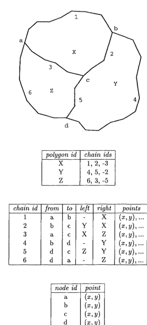
z
5 4
polygon id chain ids
x
1, 2, -3 y 4, 5, -2z
6, 3, -5chain id from to left right points
1 a b -
x
(x, y), ...2 b c y
x
(x,y), ...3 a c
x
z
(x,y), ...4 b d - y (x, y), ...
5 d c
z
y (x,y), ...6 d a
-
z
(x, y), ...node id point
a (x, y)
b (x, y)
c (x, y)
[image:14.602.168.403.146.665.2]d (x, y)
Chapter
4
Relational Database
Management Systems
A relational database management system is a program, or set of communi-cating programs, that manages relational databases. Most modern database systems in use today are relational, and most of these use a query language, such as QUEL or a form of SQL (Structured Query Language), to communicate between the user and the processor.
4.1
Data that.is handled well
Relational databases excel in applications where the data easily fits the entity-relationship model. Relational databases are well suited to the representation of entity-attribute data, and the representation of relations between entities. For example, a census database is often easily represented in a relational database. Non-spatial geographical data, such as land parcel details, is also well handled.
4.2
Data that is not handled well
4.2.1 Union-type data
However, some data is difficult to coerce into an entity-relationship form. Data that corresponds to a C-type union structure, for example, can be hard to represent. This type of structure can occur in geographical data. For example, the Spatial Data Transfer Standard defines
a point as a zero-dimensional object specifying a geometric location,
a line segment as a direct line between two points,
an arc as a locus of points that forms a curve that is defined by a mathematical function,
a chain as a directed non-branching sequence of non-intersecting line segments and/or arcs, and
a ring as a sequence of non-intersecting chains, strings and/or arcs.
As these are stored in separate tables, the rings table would require a field indicating which whether a ring-segment is a string, chain or arc, and a query to find all points in a ring R would become much more complicated, as shown in Figure 4.1.
For this reason, this representation was not considered appropriate for queries, although it is suitable for the transfer of data.
4.2.2 Sequenced data
Any data that involves some form of sequencing is not naturally represented in a relational data model. A basic assumption of the relational data model is that every record is independent of every other record. The records that a RDBMS stores in a table are defined to be completely unordered. However, there are many examples where sequencing is important. As mentioned earlier, a river has a natural order, from a set of high points to a single low point at the river's mouth. RDBMSs often allow for chronological data to be stored, and this gives some sort of natural sequencing, irrespective of the order that the data itself is stored in, with the date attribute determining the sequence. However, spatial data often has some non-chronological natural sequencing, which requires an artificial sequence attribute in order for a standard RDBMS to deal with it.
4.3
Spatial Data in a Relational Normal Form
As mentioned in the previous chapter, spatial data is often ordered. This is usually represented by adding a field to the table that links an object to its constituent parts, this field containing the relative position, or sequence number, of the part within the object.
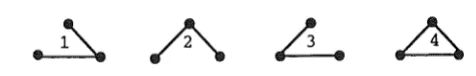
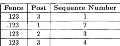
Suppose that a farmer placed three posts in a paddock, in a triangular layout, and then told his foreman to connect the posts with a fence. Without knowledge of any sequencing, there are four possible layouts that could result, as shown by Figure 4.2. In order to identify the layout as a table in a RDBMS, we would have a table containing three fields, these being the post number, the constant fence number, and the position of the post in the fence. Table 4.1 shows one possible representation of layout 4 in Figure 4.2, with three line-segments.
PosTGRES offers us an alternative to artificial sequence numbers, whereby
select* from points where points.id in (
select point_id from point_arcs where arc_id in (
select part_id from chain_parts where part_type
=
'A'and chain_id in (
select part_id from ring_parts where part_type = 'C'
and ring_id
=
R))) or points.id in (select point_id from point_linesegs where lseg_id in (
select part_id from chain_parts where part_type
=
'L'and chain_id in (
select part_id from ring_parts where part_type
=
'C'.and ring_id = R))) or points.id in (
select points_id from point_linesegs where lseg_id in (
select lsegs_id from lseg_strings where string_id in (
select part_id from ring_parts where part_type
=
'S'and ring_id
=
R))) or points.id in (select points_id from point_arcs where arc_id in (
select part_id from ring_parts where part_type
=
'A'and ring_id
=
R)))Figure 4.1: Selecting all points in a ring R using the Spatial Data Transfer Standard representation
A
[image:17.597.168.406.662.700.2]Fence Post Sequence Number
123 3 1
.123 1 2
123 2 3
[image:18.600.196.389.374.449.2]123 3 4
Chapter 5
Postgres
PosTGRES is a free, but unsupported, (and often unstable) object-oriented extended relational database management system under development at the University of California, at Berkeley. It is still in the developmental stages, even though work started in 1986. The current version is 4.2, with the department here running version 4.1. It uses its own query language, PosTQUEL, based on QUEL.
5.1
Features of
PosTGRES"Traditional relational 'DBMSs support a data model consisting of a collection of named relations, each attribute of which has a specific type. In current com-mercial systems, the most common type are floating point numbers, integers, character strings, money, and dates. It is commonly recognised that this model is inadequate for future data processing applications.
The relational model succeeded in replacing previous models in part because of its simplicity. The PosTGRES data model offers substantial additional power
by incorporating the following four additional basic constructs.
classes
inheritance
types
functions" (Rhein et al., 1993)
Classes are basically identical to tables in a relational database, but with the added ability of inheritance. Classes may inherit all of the fields and functions of one or more other (parent) classes. An item in a subclass does not need to have a entry in its parent class, so the size of the parent class can be reduced. Queries on the parent class may include all subclasses by adding an asterisk after the parent's name in the query. As an example, we could have a class of land parcels, and this would be a subclass of, and inherit the functions and fields from, the polygon class.
!- -,-,_
'
1,-User-definable types appear to be the most useful innovation. No longer .is one limited to the basic data types mentioned by (Rhein et al., 1993), above. One can now have, in theory, a 12-byte integer, picture, sound, or even movie as data types. One can even have fixed and variable length arrays of data types, including other arrays. The database owner has to provide their own definition of their data types, which must be stored as a continuous unit of memory. (That is, it must not include any pointers). Much of the advantage and power of PosTGRES lies in the array data type, which has a limited set of predefined functions. User-defined types are written in C, and have equal status with all other data types.
Given a new data type, functions must be defined to access it, including at least conversion to and from string representation for input and output. If comparisons are to be made with any data type, then functions need to be defined for this purpose. The function names must be unique and no more than fifteen characters in length. It is common to include the function argument types in the function name. The function definitions can be written in either
PosTQUEL, or
c.
Operators provide an alternative way of representing functions. The name of an operator does not need to be unique, as the operator is defined by its name and argument types. However, it was found that an operator name may not contain alphabetic characters, so that 'isin' or 'eq' are not valid function names (this was not documented). For example, 'A
=
B' can be represented by any of abstimeeq (ab~time, abstime), booleq (bool, bool), box_eq (box, box), chareq (char, char), char16eq (char16, char16), etc. This list may include user-defined functions.The operators provide a simple way in which to call a function, with-out having to remember the different function names. They also provide a means of defining what functions are the boolean inverses of each other (called negator by POSTGREs), and what functions are equivalent to another with the arguments swapped (called commutator). For example, the function called isEleminArray(elem, array) is equivalent to arrContainElem(array, elem), and in fact, the C-code for the later calls the first with its parameters swapped.
Not mentioned in this list if features, but also supported, is the notion of (historic) time travel. This allows historical data to be accessed, by supply-ing a time or range of times with the class name. For instance, to find all former addresses of a student, one could use the PosTQUEL query 'retrieve (P. address) from P in Persons[, "now"] where P. student id
=
9134567' By default, "now" is used if no time range is specified, 11 Jan 1 00: 00: 00 1970GMT" is the default if a time range is specified with no start time, and 11
now11
for the default end time. Thus, 'Persons [,"now"]' could have been replaced with 'Persons[,]' in the above example.
5.2
What should
be possible in
PosTGRESpoints in an ordered array. From this array, we have an immediate traversal order without separate sequence numbers. Thus our representation of the fence earlier can now be made in a class (table) containing one row and two columns instead of a table of three or four rows and three columns. There is an immediate saving in space here. The following shows the difference.
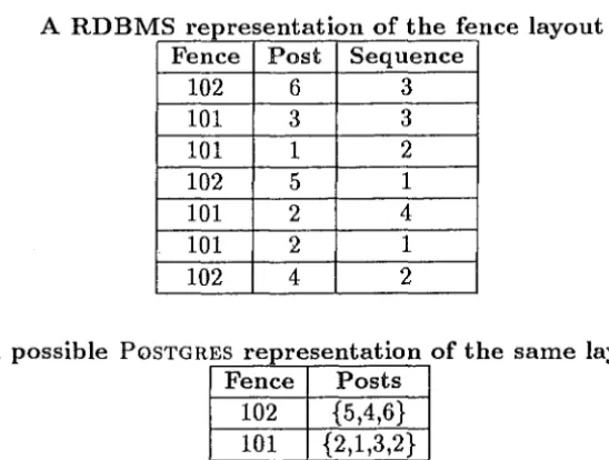
Suppose in our fencepost example, we had two fences numbered 101 and 102, and an extra set of posts numbered 4, 5, and 6. Suppose we had the first fence joining poles 2, 1, 3, 2 in that order, and the second joining poles 5, 4, 6. A comparison of the ways that PosTGRES could represent the data compared with a normal RDBMS can be seen in Table 5.1.
A RDBMS representation of the fence layout Fence Post Sequence
102 6 3
101 3 3
101 1 2
102 5 1
101 2 4
101 2 1
102 4 2
A possible PosTGR ES represen a ion of the same layout t t• Fence Posts
102 {5,4,6}
101 {2,1,3,2}
Table 5.1: RDBMS and PoSTGRES representations of the fence layout Note that there is still no concept of ordering between the rows of a table in either example.
[image:21.602.150.424.254.461.2]Chapter
6
Data Structures
This chapter looks the two different types of geographical features that were mentioned in Section 3.3. Firstly, it looks at the basic Point-Chain-Polygon model, based on ( van Roessel, 1987) 's definitions. The second structure exam-ined is a stream network. For each of these feature types, a set of possible data structures to represent a feature in PosTGRES, including a representation that would be adopted by a relational database, are examined closely. The size and efficiency of the data structures are compared. The most efficient data structure was then used in the experiments with PosTGRES.
It is assumed that four byte integers are used to represent identifiers, and eight byte floating point numbers are used to represent the coordinates of a point. Furthermore, it is assumed that coordinates only involve two dimensions, x and y. If the database holds height attributes as well, then eight more bytes will be required to represent each point.
Any overhead that the database management system requires to represent a table has been ignored for the sake of simplicity.
6.1
Points, Chains and Polygons
From (van Roessel, 1987)'s definitions given in Section 2.2, we can see that a polygon is made up of possibly many rings, each made up of many chains, and each in turn made up of many points. Nodes can be thought of as a subclass of points, inheriting the coordinate attributes. Lines are a superclass of chains, as they relax the need for start and end nodes, and they may not have a polygon on either side. We need some type of structure to represent the links between these different classes.
In the following example representations, points and chains are used, al-though the same model can equally be used for chains and rings, or rings and
polygons.
Three different models were considered to represent the links ( or joins) be-tween the classes, and were then compared for efficiency for different types of queries, and their overall representation size. These models were:
same way that a relational database would. This requires three separate tables, namely
- Points, consisting of the point identifier, and the x and y coordinates of the point;
- Chains, consisting of the chain identifier, and the identifiers of the polygons on the left and right side of the chain; and
Points_Chains, consisting of list of points that are in each chain, and represented as a point identifier, chain identifier, and the sequence number of the point within the chain.
Given c chains, p points, and
t
total point/chain pairs, this representation requires 12c+
20p+
12t bytes to represent it.• Representation B - We could replace the Points_Chains table of rep-resentation A with an extra attribute of Chains. This extra attribute would be an array containing an ordered list of the points that make up the chain. PosTGRES supports to a certain degree the use of arrays as a base data type, but it requires that any variable length array contain in the first four bytes the number. of bytes for this instance of the array.
This representation requires 16c
+
20p+
4t bytes to represent it, being 20p bytes to represent the points table, 12c bytes to represent the chain identifier and the two polygon identifiers for each chain, 4c bytes to store the length of each instance of an array of point numbers, and 4t bytes representing the fact that each point/chain pair is stored only as a single 4-byte integer in the points attribute of the chains table.This representation allows quicker execution of queries like 'Find the end
points of this chain', and is the fastest overall representation for adding, deleting, and updating the links between the classes.
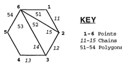
2
4 13 3
1-6 Points
11-15 Chains
51-54 Polygons
Figure 6.1: A Sample Point and Chain Network
• Representation C - One major problem with representation B is that it requires O(t) processing time to answer the queries "Find all chains
[image:23.600.188.390.529.638.2]per-Table of Points
Po in Lid x y Chains
1 3 4 {11}
2 4 2 {11,12,15} 3 3 0 {11,13,14}
4 1 0 {13}
5 0 2 {13}
6 1 4 {13,14,15,11}
Table of Chains
Chain_id LefLPoly RighLPoly Points
11 54 51 {6,1,2}
12 54 52 {2,3}
13 54 53 {3,4,5,6}
14 53 52 {3,6}
15 51 52 {6,2}
Table 6.1: Representation .C of the example point and chain network
representation A. This O(t) time requirement is not acceptable if these queries are to qccur. This problem can be solved by adding an extra attribute to points - an unordered array of all the chains in which the point occurs. The two queries are then reduced to O(logp) and O(logpc) respectively, although a penalty is accepted by having some (O(logp)) extra delay in adding, updating, and deleting links between chains and points, and also when deleting a chain.
This representation requires the use of 16c
+
l6p+
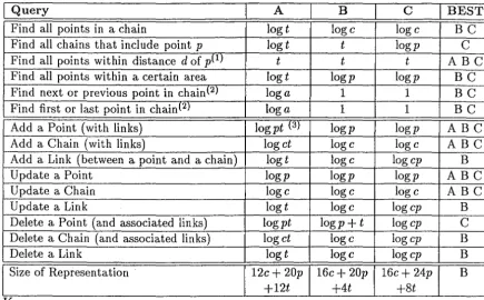
8t bytes, which is still below that of representation A. An (unrealistic) example is given in Figure 6.1 and Table 6.1.A comparison of the three representations is given in Table 6.2. Although at first representation B appears to be the best overall, an examination of the two cases where it is not the best proves it to be totally unsatisfactory. If we have a database with one million points, then a query to find all chains includ-ing a certain point usinclud-ing representation C or A would only require about 20 comparisons, while representation B would require in the order of 106
compar-isons. If one of these queries took 1.5 seconds using representation C, it would take around a day using representation B. This is clearly unacceptable for these cases.
I
Query A Bc
Find all points in a chain log t loge log c
Find all chains that include point p log t t logp Find all points within distance d of p<1> t t t
Find all points within a certain area logt logp logp Find next or previous point in chainl2J log a 1 1
Find first or last point in chainl2J log a 1 1
Add a Point (with links) logpt <3> logp logp
Add a Chain (with links) log ct loge log c
Add a Link (between a point and a chain) log t loge logcp
Update a Point logp logp logp
Update a Chain loge loge log c
Update a Link log t loge logcp
Delete a Point (and associated links) log pt logp + t logcp Delete a Chain ( and associated links) log
ct
loge logcpDelete a Link log t loge logcp
Size of Representation 12c + 20p 16c+ 20p 16c+ 24p
+12t +4t +st
Key
• a - The average number of points per chain
411 c - The number of chains in the database
• p - The number of points in the database (that is, the total number of records in the points and nodes classes)
• t -
The total number of chain/point pairings, that is, the number of entries in the Chains..Points table in a relational representation.• Note 1 - This could be reduced by preceding it with a query that selected those points with Px-d:::; x_coord:::; Px+d and Py-d ~ y_coord ~ Py+d.
• Note 2-For these queries, it is assumed that a query has already retrieved all points in the chain into a separate table or class. If this is not the case, then the complexities are log a+ log t = log at, log c, log c respectively. e Note 3 - This is equal to logp + log t, and represents adding one record
to the table of points, and on average a records to the table of links (Chains..Points). The number of links added has a linear effect. (O(logt) for the first link, 0(1) thereafter.)
Table 6.2: Time and space complexities of the three different methods of rep-resenting links between points and chains.
I
BESTI
[image:25.602.100.536.125.395.2]6.2
Network Structures
Four different data structures for storing and manipulating a network structure were examined. These four data structures fell into two categories,
1. storing a whole river network as one single structure, or
2. storing the data in a form equivalent to a relational database representa-tion.
These four data structures were then compared for their calculated time and space complexities for some typical queries, and any limits on the total size of the network imposed by the suggested data structure.
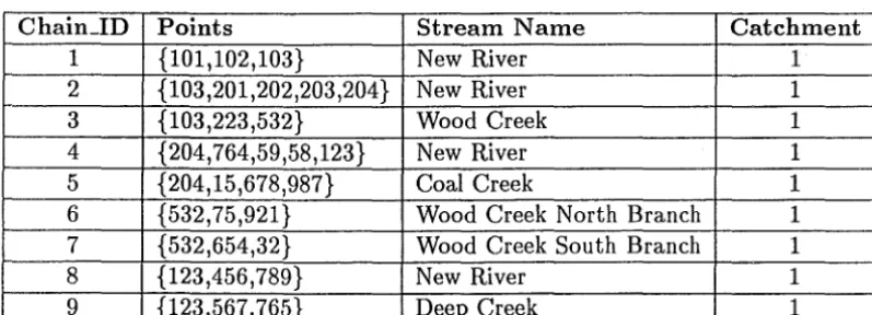
Figure 6.2 shows a sample river network, flowing west towards stream section 1, to show the different methods of representation. It is assumed that for all representations, there is a class (Rivers) of all chains that make up a stream section. These chains have chain_ids as shown in Figure 6.2. This class ( a subclass of chains) can be seen in Table 6.3, and has the following structure:
• ChainJd - the unique number referring to the stream section.
• Points - a list of the points that make up the stream.
• Stream..N ame - a fixed length string of characters defining the stream name of this section.
• Catchment - The unique chain_id referring to the mouth of the river.
The first three representations represent the network as a binary tree, that itself has been represented as an array to remove any pointers. The data is stored in pre-fix mode, with the downstream chain from an intersection (node) specified, then the whole left-hand branch, then the whole right hand branch. Here the terms left-hand branch and right-hand branch refer to the two upstream branches of the stream ( or river) as one stands at the intersection of two streams, and faces upstream between the two contributries.
For example, the river network in Figure 6.2 would be represented by the sequence {1,{2,{4,8,9},5},{3,6,7}}. The three representations differ in the way in which they internally represent the structure of the network. As mentioned earlier, POSTGRES requires that the first four bytes of a variable length data
type are used to store the length (in bytes) of the data structure.
In order to display a stream, including its contributries, it is necessary to search a stream upstream from the current point, to find all of the chains that make up the stream, and the points that make up these chains. In other cases, it may be required to find all points downstream from from the current location, for example, in the case of water pollution. Most queries however, will be of the form "show the streams within these coordinates", which is equivalent to "show
all chains that are of type 'stream' and are within these coordinates". This
8 9
7
Figure 6.2: A Sample River Network
Chain_ID Points Stream Name Catchment
1 {101,102,103} New River 1
2 {103,201,202,203,204} New River 1
3 {103,223,532} Wood Creek 1
4 {204,764,59,58,123} New River 1
5 {204,15,678,987} Coal Creek 1
6 {532,75,921} Wood Creek North Branch 1
7 {532,654,32} Wood Creek South Branch 1
8 {123,456,789} New River 1
[image:27.600.101.500.493.637.2]9 {123,567,765} Deep Creek 1
appear in the Rivers subclass of Chains, the requirement for a stream network representation is to be able to answer the upstream/downstream queries.
The four representations examined were:
• Representation A - The top bit of a chain_id is set to indicate a non-terminal node. This obviously allows for only 231 chain_ids, although this is not a great restriction. When a chain is read with the top bit set, the top bit is removed to get the chain identifier's value, and then the level ( distance in nodes from the root of the tree, or intersections from the river mouth) increases by one. The next two chain....ids at the same level represent the two branches of the river network at that point. After reading the two branches, (for example, 4 and 5) the level is decreased by one, and the next chain read is at a lower level (for example, 3). This is the most space-efficient representation, requiring only 4 bytes ( the size of a chain....id) for each stream section. Searching up the left stream is fast, but to search up the right stream requires the whole of the left stream to be read first. Searching downstream is also slow, as we must read backwards through the whole left hand branch of an node if we are at the base of the right hand branch of that node.
For example, from location 2, we can tell that the previous stream in the sequence (1) has its top bit set, so it is a non-terminal, and so is the node immediately downstream of 2. However, from location 3, the immediately previous stream, recorded was 5, which we can tell is a terminal node, and so we must be at the base of a right hand branch, looking at a leaf of the left hand branch. These leaves have to be paired off until we get back to stream 2, who's predecessor was 1, which is immediately downstream of
3.
• Representation B adds a four-byte integer before each non-terminal node. The top bit is set, to indicate a non-terminal is following, and the remaining 31 bits give the position within the structure of the downstream node. Again this allows us to use only 31 bits for the chain_ids, and searching downstream is very fast (0(1), if the whole array has been retrieved already). As half of the stream sections are non-terminal, we have an average 2 bytes extra space required per stream section, making an overall average of 6 bytes per stream section.
• Representation C adds another four-byte integer before the non-terminal stream section, this indicating the position of the stream section definition of the right incoming stream. (The immediate left hand stream starts at the next chain in the sequence, so it does not need its location stored.) This changes the time complexity of reading downstream and upstream to 0(1), and requires an average of 8 bytes to represent each stream section.
For example, Figure 6.2 would be represented as in Table 6.4.
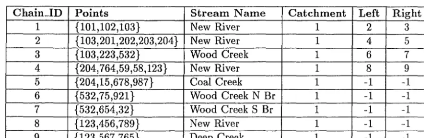
extra field giving the first stream of the left and right branches. It does not need any special data structures to be developed.
It allows all fields (except points) to be indexed, to speed up accessing. This gives O(t) time response to queries involving finding the next stream either upstream or downstream, searching by river name, or by chain_id, where t is the total number of stream sections (records) in the class. Continuing our example, Figure 6.2 would be represented as in Table 6.5.
Position size 0 1 2 3 4 5 6 7
Value 72 -1 * 12* 1 O* 11 * 2 2* 10* '.· ~ ·~~-.:
Position 8 9 10 11 12 13 14 15 16
Value 4 8 9 5 O* 16* 3 6 7
* Highest bit set to 1 to indicate a position rather than a value.
Table 6.4: Network Representation C - Array with Two Pointers
Chain_ID Points Stream Name Catchment Left Right
1 {101,102,103} New River 1 2 3
2 {103,201,202,203,204} New River 1 4 5
3 {103,223,532} Wood Creek 1 6 7
4 {204,764,59,58,123} New River 1 8 9
5 {204,15,678,987} Coal Creek 1 -1 -1
6 {532,75,921} Wood Creek N Br 1 -1 -1
7 {532,654,32} Wood Creek S Br 1 -1 -1
8 {123,456,789} New River 1 -1 -1
9 {123,567 ,765} Deep Creek 1 -1 -1
[image:30.602.142.437.193.269.2] [image:30.602.98.532.483.625.2]/ Query A B
c
D BestWhich river is this chain in? logt log t logt log t ABCD Which chains form this river? log t logt log t log t ABCD
Which node is next downstream? c 1 1 log t BC
Which node is next upstream to the left? 1 1 1 log t ABC Which node is next upstream to the right? u u 1 log t
c
All points downstream le l l l logt BC
All points upstream u u u ulogt ABC
Maximum number of chains 231 231 231 232
Maximum chain_id 231 231 231 232
I
Size of representation 4t 6t 8t 8tKey
• c - Number of chains (streams) that make up this river network.
e l - The current level in the river network, that is, the number of stream junctions between this point and the river mouth.
• n - The total number of river networks (that exit to the sea or lake).
• t - The total number of chains in all river networks, which can be approx-imated by nc. This is the number of rows in the streams table.
• u -The number of streams upstream of this point, which can be approx-imated by c/2'.
Table 6.6: Time and space complexities of the four different methods of repre-senting a river network.
D D
A
[image:31.598.102.517.232.399.2]Chapter 7
Postgres
Implementation
Issues
In order to test the suitability of PosTGRES for representing geographical data, it was necessary to set up a small sample database, and to carry out some experiments with this data. From the previous chapter, we have a method of representing stream networks, and a Point-Chain-Polygon model. This chapter discusses the issues involved in putting the theory into practice.
The first section deals with the design of a basic Geographical Information System. This system contains the core elements that are needed for a sys-tem, namely an implementation of the basic zero, one, and two dimensional geographical features, and some subclasses of these. Furthermore, it contains an implementation of a stream network, and allows the user to select data by layers.
The second section deals with the functions and operators that are needed to effectively use the major classes (Points, Chains, and Polygons) that have been set up. It also provides some PosTQUEL queries to execute queries on these classes.
The third section looks at the required functions and operators to use the stream networks effectively. An example PosTQUEL query is provided to find the names of all rivers and streams that flow into a given river.
The fourth section of this chapter looks at the method used to collect and enter the geographical data into the PosTGRES database.
Finally, the fifth section deals with the numerous problems that were en-countered when using PosTGRES. Some of these problems can be easily solved by applying publicly available patches to the PosTGRES program itself; others can be solved by applying patches to the data. However, a number of intermit-tent bugs still remain.
7 .1
The design of a sample Geographical
Informa-tion System
Class Field Type Key in
I
Indexed?I
Entities id int4 Primary Yes
sub_class char Non-key Yes
layers int_array Non-key No
Layers id int2 Primary Yes
description text Non-key No
entities int-array Entities No
Points x floats Non-key Yes
y floats Non-key Yes
chains int-array Chains No
I
NodesChains LPoly int4 Polygons Yes
RPoly int4 Polygons Yes
points int_array Points No
Rivers name text Non-key Yes
catchment int4 Catchments Yes
l
Roads . namel ·
text Non-key YesI
Rings chainsI
int-arrayI
Chains NoI
Polygons chainsI
int-arrayI
Chains NoParcels · parceUd int4 Primary Yes
flat..number int2 Non-key No
st..number int2 Non-key No
stJetter char Non-key No
st..name text Non-key Yes
suburb char16 Non-key Yes
town char16 Non-key Yes
Catchments rivers
I
int_arrayI
Rivers NoNotes
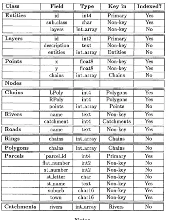
• The Nodes class contains exactly the same fields as the Points class, and the records form a subset of the Points* extended class.
• The Key in column contains one of three values,
Primary, to indicate that the field forms the primary key; Non-key, to indicate that the field does not form a key; or
a class name, to indicate that the field contains a foreign key reference to the given class.
[image:33.600.121.475.97.548.2]The model used here is based on that proposed in (van Roessel, 1987) after some problems were encountered with some of the other models, which had the concept of unions, as mentioned in sub-section 4.2.1.
van Roessel defined spatial objects using the terms shown in Section 2.2, and these are the definitions that have been used in this report.
The sample database that was set up includes the major classes Points, Chains, and Polygons, with subclasses nodes (inheriting the fields and func-tions of Points), parcels (inheriting from Polygons), and roads and rivers (inheriting from Chains). A minor class catchments has been set up, which holds the whole stream network for every river or stream that exits into a body of water (ocean, sea or lake).
Class Layers contains for each coverage layer (numbered from O to 65535) a list of all entities that occur in that coverage layer, and a textual description of that coverage layer, such as "Road", "Drainage", "Building" and "River". Finally, class Entities has been implemented as a superclass of the Points, Chains, Rings, Parcels and Catchments classes. This class is actually empty, with all of its records held in its subclasses. The attributes of Entities are a unique identifier for every entity, a character indicating the subclass that the entity appears in (for queries on Entities*), and a list of the layers that the entity appears in.
The database from which the sample data was obtained, dpdb, did not hold
any lines that were not chains, and so the lines class was eliminated. There were five cases of polygons containing interior rings in the whole dpdb database,
although none of these cases occurred in the Cashmere section of the database, from where the sample data was obtained. It was decided to keep the Rings class, but not to implement a link from Chains to this class, due to its infrequent usage.
There is a link from Polygons to Rings, provided by the rings attribute in Polygons, and this attribute contains an array of just one element in all of the sample cases, although on occasion this array would be larger. There is also a link from Rings to Chains, providing an effective link from Polygons to Chains. The reverse link (from Chains to Polygons) is provided by the LPoly and RPoly attributes of Chains. Thus, there is no loss in efficiency by not providing a link from Chains to Rings, and the representation is more compact.
Table 7 .1 shows the class definitions.
The data types used were int2 (for anything with a maximum value less than 65535), int4 for most identifiers, int....array for arrays of int4, floats for geographical coordinates, char for single characters, char16 for any attributes that are always under 16 characters in length, and text for text strings of longer strings. All of these, apart from int_array, are provided in PosTGRES by
default. However, any set length character strings other than those of length 1 or 16 (such as char(n) in SQL) must be explicitly defined in C, and appropriate functions to convert from strings to the storage representation, and back again, also need to be defined. In many cases it is easier to use the general purpose text type, unless we can be fairly sure that the values are all less than 16 characters. text has been used for road names, as these can be longer than 16
characters, an example being Sir William Pickering Drive in Burnside.
It was decided to index those attributes that formed a link between classes, (apart from the attributes of type int_array, which cannot be indexed) as well as the attributes that would be used in common queries, such as x and y coordinates, street names, suburb and town names, as well as fields that form a primary key of a class.
7.2
Representing the Major Classes
The next question considered was what types of queries would be the most common and, therefore, what types of queries should our database structure easily support. These were considered to be queries such as "Find all points on
this chain or polygon", "Find all polygons that include this poinf', "Find the polygons that border this chain", and "Find all points/polygons that are within
a certain distance of this point/polygon"
Ideally, given the above queries, and the design in the previous section, it was desirable to be able to generate queries equivalent to the following SQL:
select* from Points where pointid in (
select points from chains where chainid in ( select chains from rings where ringid in (
select rings from polygons where polygonid
=
123)));The SQL operator 'in' operates on an expression and a list of expressions. That is, the syntax of 'in' is 'y in (x, ..• , z) ', which is equivalent to 'y = x
or . . . or y = z'. The alternative version of 'in' has syntax 'expression [not] in (subquery) ', where subquery returns exactly one column. (Rela-tional Technology Inc, 1990)
Ideally, one would like to use an operator that is a combination of these, with the list (x, ... , z) replaced with an array. That is, the sub-query 'select rings from Polygons ... ' would return exactly one field, or column, from Polygons, and each element in this field would contain an array of values, each of which is to be compared with the left hand side of the operator. Furthermore, it would be hoped that such an operator would not match the first four bytes of a variable length array, as these bytes contain the array length, and not data. (PosTGRES also has a reserved word 'in', but it has a different meaning to the SQL in reserved word, as can be seen by the PosTGRES query below, and so is not suitable.)
Unfortunately, PosTGRES does not appear to provide a way of detecting if a given value is in a general position in the array. If there is a way, then it is not mentioned in the PoSTGRES User Manual (Rhein et al., 1993) or in the PosT-GRES Reference Manual (The Postgres Group, 1993). The only documented support provided for arrays is the ability to define them, enter and retrieve them in their entirety, or to be able to access a specific location. Furthermore, the basic structure of the array as it is stored in C was not documented, mak-ing it harder to implement this function in C directly. Eventually some source
I
I·-·
code was found that defined the array, which made it possible to build the C functions required.
The function that was required to detect if an element is in an array was called isEleminArray(elem, array), which returned true or false. This has an associated operator, @, which is used as elem © array. Related to this op-erator are opop-erators!@ (for elemNotinArray),"' (for arrContainElem), and!"'
(for arrNotContElem). The names chosen for the functions follow PosTGRES's restriction of a maximum of fifteen characters in the function name. @ and "' were used, because they are currently used by PosTGRES for "A is contained
in B'' and "A contains B'' respectively, where A and B are boxes or polygons. Once this was defined, it was possible to rewrite the query "Find all points
that form the border of polygon number 12:J' into PosTQUEL, as:
retrieve (p.id) from pin Points, c in Chains, r in Rings, poly in Polygons where p.id © c.points
and c.id © r.chains and r.id © poly.rings and poly.id= 123
Likewise the query "Find all polygons that include point 456" could be writ-ten as:
retrieve (poly.id)'from pnt in Points, chn in Chains, poly in Polygons
where (poly.id= chn.LPoly or poly.id= chn.RPoly) and chn.id © pnt.chains
and pnt.id
=
456Finally, a query of the form "Find all points that are within 100 metres of
point 456' is slightly more tricky to deal with. It can be answered given a
new function distance, which takes the x and y coordinates of two points, and returns the distance between them. This enables the query to be written into PosTQUEL as:
retrieve (pnt.id) from pnt in Points, Pin Points where distance(pnt.x, pnt.y, P.x, P.y)
<=
100and P . id
=
456I*
First, clear any old points from the ClosePoints class*I
delete ClosePoints \gI*
Then append to ClosePoints all points within a 200m x 200m*
box around point 456*I
append ClosePoints (pnt.all) from pnt in Points, Pin Points where pnt.x >= P.x - 100.0and pnt.x <= P.x + 100.0 and pnt.y >= P.y - 100.0 and pnt.y
<=
P.y + 100.0 and P.id = 456 \gI*
Finally, execute the retrieve on the ClosePoints class*I
retrieve (pnt.id) from pnt in ClosePoints, Pin ClosePoints where distance(pnt.x, pnt.y, P.x, P.y)
<=
100and P.id
=
456 \g(\g is the 'go' command in the PosTGRES terminal monitor.) Most other queries can be answered just as simply as these examples.
7.3
Representing Stream Networks
Streams are represented by having a class Rivers which is a subclass of Chains, with the extra fields name and catchment. A further class, Catchments contains a catchment identifier id and a network structure rivers consisting of the rivers and streams that make up the catchment. These allow queries like "Find all
streams flowing into the Bealey Rive'F' to be executed quickly, as a search of the Rivers class (which contains an index on the river name) gives us the chain numbers that make up the Bealey River, and also specifies that it occurs in the Waimakariri River catchment. By looking up the Waimakariri catchment (in the Catchments class), and using some predefined C functions, the section of the Bealey that exits directly into the Waimakariri River can be found, and the identifier for this stream section (or chain) is returned (that is, the first occurrence of any of the chain numbers that make up the Bealey River, in the Waimakariri River catchment network).
By then using alLup_stream, the whole Bealey River sub-catchment is returned, and by using stream2array, this can be converted into a list of all chains that make up the the Bealey River sub-catchment. Finally, a query can be made to return the unique names of all rivers that have an identifier in the list of chains, such as the Minga River, and the Punchbowl, Rough and Avalanche Creeks.
from river in Rivers,
I*
The streams that flow into the Sealey*I
catchment in Catchments,I*
The Waimakariri River Catchment*I
exit in Rivers,I*
The most downstream part of the Sealey,*I
I*
where it exits into the Waimakariri*I
target in RiversI*
All chains that make up the Sealey,*I
I*
but no contributries*I
where river.id© stream2array(all_up_stream(catchment.id, exit.id)) and exit.id© sub\_catchment(catchment.id, target.id)
and catchment.id= target.catchment and target.name= "SEALEY RIVER"
Various functions have been defined for network data structures, other than the required conversions to and from character strings. Briefly, these are:
• down...stream - to return the chain identifier of the stream section that is immediately downstream from the stream section supplied.
• lup...stream - to return the chain identifier of the stream section that starts the left hand branch upstream from the stream supplied.
• rup...stream - to return the chain identifier of the stream section that starts the right hand branch upstream from the stream supplied.
• alLdown_stream - to return an ordered list of all stream sections that are downstream' of the stream supplied.
• alLup_stream - to return the full stream network of all points that are upstream of the current location.
• stream2array - to convert a stream network into a list of the chains that make up the stream.
• sub-catchment - supplied a catchment and a list of chain identifiers of all stream sections with a given name, returns a list of ( usually one) downstream-most occurrence of an entry in the supplied list. The only time that more than one occurrence may be returned is when a catchment contains more than one stream with the same name (for instance, two
Rough Creek's in the whole Waimakariri River catchment).
7.4
Importing the Data
allows only one query to be executed at a time in this manner, and as each entry and exit from the monitor takes about 2 seconds, this is a very long task for a large database. The third way is to use the PosTGRES monitor com-mand copy, which allows data to be copied directly between a UNIX file and a specified class. The PosTGRES Reference Manual (The Postgres Group, 1993) warns that "Copy has virtually no error checking, and a malformed input file
will likely (sic) cause the backend to crash. Humans should avoid using copy
for input whenever possible." Despite this, no suitable alternative to copy is
provided by PosTGRES, and so it was decided to risk using it to load the data, and no problems were encountered. The author assumes that error checking will be added to future versions of copy, and this will provide a quick, yet safe, method of transferring classes between the database and UNIX files.
This solves the problem of getting the data into the database, but not the problems of collecting it in the first place, and of converting it into the representation required. The data was obtained by running suitable queries on the department's INGRES geographical database dpdb. The resulting tables were then copied into a text file using INGREs's copy command.
In INGRES, the SQL select syntax allows tables to be selected and displayed in a user-defined order. However, the copy command uses sub-select to collect the data to be exported to a file, and the sub-select syntax does not allow ordering. It is important in the next step that where, for instance, a chain is made up of a sequence of points, these points are grouped together in the file, and in the correct,sequence. For this to occur, each row in the file that is copied from INGRES must start with the field's chain and sequence, so that the resulting file can be piped through sort ( 1) to achieve the ordering required. After piping through sort, the sequence number is no longer needed.
The file is then piped through a program called rows2array that converts all sets of consecutive rows in the original that have an identical chain number (remembering that the original is now sorted by chain number) into a single row with a comma separated list of points. At the same time, it removes the sequence number from the data. The rows2array command takes two or three arguments, each argument referring to the position of a field within the data. The arguments are the positions of the primary and secondary keys of the source file, and an optional field to be removed from the source.
The resulting file should now be in a form acceptable to be loaded into a PosTGRES class, if it wasn't for a small bug that was introduced into version 4.0.1. An unsuccessful attempt by the PosTGRES programmers was made to remove this bug in version 4.1. This bug results in the character representation of an array of one item being treated as an empty array, causing the loss of this data. The hack that has been found by the programmers to work is to quote any single element in an array, and this is done by piping through a second program written by the author, pgbugfix.
In summary, the steps involved in copying INGRES points, chains, and poly-gons, etc to PosTGRES are
• Run a query in INGRES to select the data required into a table.
i-·
taking particular note to the file order.
• Pipe data. igs through one or more of sort, rows2array and pgbugf ix to make a file data. pgs, remembering to specify the key fields to rows2array.
• Create a class in POSTGRES that has identical fields and field types to data.pgs.
• Use copy from PosTGRESjs monitor program to copy the data from data. pgs to the new class.
7.5
Problems encountered with
PosTGRESPosTGRES is only an experimental database, and it is well known for the nu-merous bugs that it contains. The following is a summary of the bugs, undocu-mented features, docuundocu-mented but non-existent features, and general problems found while experimenting with POSTGRES.
1. The monitor (frontend) would crash unexpectedly. This would often occur if there was an error in the query, such as a mistyped function name. Within a second
of
the query being issued, the following error would be reported, and the monitor would exit.Error: No response from the backend, exiting ...
2.
-c
was used to stop a processing query, and this is also used to force the monitor program to exit. Unfortunately, this meant that monitor would exit whenever a query needed to be cancelled.3. If the frontend crashes, or is aborted, the backend continues unsuccessfully trying to process the query. On one weekend, the frontend crashed many times, each time leaving query being processed on the department's main computer, huia. Each of these added about 2 units to the load on the main computer (according to top ( 1) ), which promptly became overloaded and therefore slowed down considerably, with a load of about 36 units. As this was a Saturday, the problem was not fixed until Monday, and all users over the weekend suffered from slow responses.
4. Query optimisation is not carried out, except to include the effects of any user-defined rules. However, the order of the restrictions in a query was found to greatly influence the length of time taken for it to execute. An example is the following query:
retrieve (pnt.id)
from pnt in Points, chn in Chains, rng in Rings, ply in Polygons