Multiresolution image modelling and estimation

(1)

warwick.ac.uk/lib-publications

A Thesis Submitted for the Degree of PhD at the University of Warwick

Permanent WRAP URL:

http://wrap.warwick.ac.uk/109834

Copyright and reuse:

This thesis is made available online and is protected by original copyright.

Please scroll down to view the document itself.

Please refer to the repository record for this item for information to help you to cite it.

Our policy information is available from the repository home page.

(2)

T H E B R IT I S H L I B R A R Y D O C U M E N T SUPPLY CENTRE

TITLE

MULTIRESOLUTION IMAGE

...

MODELLING AND ESTIMATION

A U T H O R

_{Simon Clippingdale B.Sc.}

IN STITU TIO N

and DATE

The University of Warwick

Attention is drawn to the fact that the copyright of

this thesis rests with its author.

This copy of the thesis has been supplied on condition

that anyone who consults it is understood to recognise

that its copyright rests with its author and that no

information derived from it may be published without

the author’s prior written consent.

T H E B R IT IS H L IB R A R Y D O C U M E N T SUPPLY C EN T R E

Ic m s 1 W est Yorkshire_{United Kingdom} _{R E D U C T IO N X ...}

(3)

MULTIRESOLUTION IMAGE

MODELLING AND ESTIMATION

Simon Clippingdale B.Sc.

A thesis submitted to

The University of Warwick

for the degree of

Doctor of Philosophy

(4)

M u ltireso lu tio n Im age M o d e llin g and E stim atio n Simon Clippingdale B.Sc.

A thesis submitted to The University o f Warwick

for the degree of Doctor of Philosophy

September 1988

Summary

Multiresolution representations make explicit the notion of scale in images, and facilitate the combination o f information from different scales. To date, however, image modelling and esti mation schemes have not exploited such representations and tend rather to be derived from two- dimensional extensions of traditional one-dimensional signal processing techniques. In the causal case, autoregressive (AR) and ARMA models lead to minimum mean square error (MMSE) estimators which are two-dimensional variants of the well-established Kalman filter. Noncausal approaches tend to be transform-based and the MMSE estimator is the two- dimensional Wiener filter. However, images contain profound nonstationarities such as edges, which are beyond the descriptive capacity of such signal models, and defects such as blurring (and streaking in the causal case) are apparent in the results obtained by the associated estimators.

This thesis introduces a new multiresolution image model, defined on the quadtree data structure. The model is a one-dimensional, first-order gaussian martingale process causal in the scale dimension. The generated image, however, is noncausal and exhibits correlations at all scales unlike those generated by traditional models. The model is capable of nonstationary behaviour in all three dimensions (two position and one scale) and behaves isomorphically but independently at each scale, in keeping with the notion of scale invariance in natural images.

The optimal (MMSE) estimator is derived for the case of corruption by additive white gaussian noise (AWGN). The estimator is a one-dimensional, first-order linear recursive filter with a com putational burden far lower than that of traditional estimators. However, the simple quadtree data structure leads to aliasing and 'block' artifacts in the estimated images. This could be overcome by spatial filtering, but a faster method is introduced which requires no additional multiplications but involves the insertion of some extra nodes into the quadtree. Nonstationarity is introduced by a fast, scale-invariant activity detector defined on the quadtree. Activity at all scales is combined in order to achieve noise rejection. The estimator is modified at each scale and position by the detector output such that less smoothing is applied near edges and more in smooth regions. Results demonstrate performance superior to that o f existing methods, and at drastically lower computational cost. The estimation scheme is further extended to include anisotropic processing, which has produced good results in image restoration. An orientation estimator controls anisotro pic filtering, the output o f which is made available to the image estimator.

Key W ords

(5)

Acknowledgments

This work w as conducted for the first year at th e Department o f Electronic Engineering, University o f Aston and subsequently at the Departm ent o f Com puter Science, Univer sity o f W arwick. I should like to thank the s ta ff and research workers o f both Depart ments, and particularly the Image and Signal Processing Group at W arwick (Andy Cal- way, Roddy M cColl, Ed Pearson, Martin Todd) fo r their interest and encouragement.

Thanks also to Professor Graham Nudd and the VLSI Signal Processing Group at W arwick for their patience during the final stages.

The design o f the quadtrature filtering scheme fo r orientation extraction is based largely on the work o f Dr. Hans Knutsson.

(6)

CO N T E N T S

CHAPTER 1 INTRODUCTION 1

1.1 Introductory Remarks 1

1.2 The Estimation Problem 2

1.3 Image Models 5

1.4 Least-Squares Estimation o f Images 9 1.5 The N ature o f Images and o f Vision 10 1.6 Limitations o f Least-Squares Image E stim ation 12 1.7 Principal Modifications to the Least-Squares Method 14

1.8 Thesis Outline 15

1.8.1 T he Image Model 15

1.8.2 The Estimator 16

1.8.3 Generalisation to Vector D ata 16 1.8.4 Further Modifications M otivated b y Vision 16 1.9 Experimental and Display Conditions 17

CHAPTER 2 QUADTREE STRUCTURE A N D NEW IMAGE M ODEL 18

2.1 Motivation 18

2.2 Quadtree Structure and Applications 23

2.2.1 Quadtree Structure 27

2.2.2 Ancestor and Descendant Sets 28

2.3 A New Image Model 29

2.4 Properties o f the Model 31

2.4.1 Noncausality 31

2.4.2 Scale Invariance 31

2.4.3 Correlation Properties 33

2.4.3.2 Long-Range Structure 37 2.4.3.3 Dyadic Shift Invariance 38 2.4.4 Analogy with Fractal Surfaces 38

2.4.5 Range o f the Model 39

(7)

2.6 Comments on the M odel-Generated Exam ples 41 2.7 Digital Filtering Interpretation o f the M odel 42

2.8 Correlation Transforms 42

2.8.1 Hadam ard Transform 43

2.8.2 H aar Transform 45

2.9 Implications o f the Model for Estimation 47

2.10 Generalisations 48

2.10.1 Generalisation o f the M odel 48 2.10.2 Generalisation to N-D im ensional Signals 49

CHAPTER 3 TH E ESTIMATOR 53

3.1 Problem Statem ent 53

3.2 LM M SE Estimation and the O rthogonality Principle 54 3.3 Kalman Estimation and Innovations 55 3.3.1 Causal Prediction on Increasing Data Support 55 3.3.2 Kalman Estimation in W hite N oise 58 3.4 Corruption by Additive W hite Gaussian Noise 64 3.4.1 The Model for the Noisy Im age 65 3.5 Data Sets and Vertical Operations 66 3.6 The Average-Value Data Quadtree 67

3.6.1 Correlation Properties 68

3.6.2 T he Optimal Upward E stim ator 70 3.7 The General Optimal Estim ator 72 3.7.1 Definition and Proof o f O ptim ality 74 3.7.2 Estimation o f the Root N ode 76 3.7.3 Estimation o f the Innovations Process 76

3.7.4 Summary 80

3.7.5 Digital Filtering Interpretation o f the Estimator 81

3.8 Computational Burden 82

(8)

CHAPTER 4 ADAPTATION O F TH E ESTIM ATOR TO V ISU AL CRITERIA 91

4.1 M otivation 91

4.2 Reduction o f Blocking and Alias D istortion 93 4.3 Examples o f Images Estimated with Interstitial Nodes 97 4.4 Edge Preservation — Motivation 99 4.5 A Fast Vertical Edge Detector 102 4.5.1 Tw o Indices o f Local Image Activity 103 4.5.2 Use o f Weighted G eometric M ean for Noise Rejection 105 4.6 The Spatially-Variant Form o f the Estim ator 107 4.7 The "Signal-Equivalent" Spatially-Variant Model 109

4.8 Edge D etector Examples 111

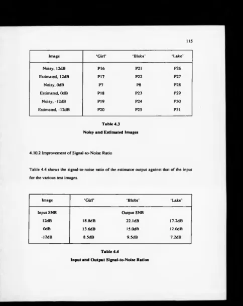
4.9 Advantages o f the Edge Detector 113 4.10 Estimation Results for the Full Implem entation 114 4.10.1 Examples of Estimated Im ages 114 4.10.2 Improvement o f Signal-to-Noise Ratio 115

4.10.3 Discussion o f Results 116

CHAPTER 5 VECTOR ESTIMATION A N D ORIENTATION 121

5.1 M otivation 121

5.2 Extension to V ector Data 123

(9)

CH APTER 6 QUADTREE A NISOTROPIC ESTIM ATION 154

6.1 Motivation 154

6.2 Quadtree Restoration o f N oisy Orientation Estimates 156 6.2.1 Examples o f Restored Orientation Estimates 157 6.2.2 Mean Squared V ector Error 157

6.3 Anisotropic Filtering 158

6.3.1 Design o f the F ilter 159

6.3.2 Examples o f Anisotropically Filtered Images 162 6 .4 Anisotropic Extension o f the Quadtree Estimator 163 6.4.1 Form o f the M odified Estimator 163 6.4.2 Directed E nergy as a Control Parameter 164

6.5 Results 164

6.5.1 Examples o f Estim ated Images 165 6.5.2 Improvement o f Signal-to-Noise Ratio 166

6.5.3 Discussion 167

CHAPTER 7 CONCLUSIONS AND FURTHER W ORK 169

APPENDIX 1 Derivation o f the Estimator by a Levinson-Type Recursion 183

APPENDIX 2 The Kalman Innovations o f the Data and the Optimal Estimator 189 A2.1 The Kalman W hitening F ilter 189 A 2.2 Derivation o f the E stim ator by Analogy with Section 3.3.2 192 A 2.3 Cholesky Factorisation o f the Data Correlation M atrix and its Inverse 197

APPENDIX 3 Probability D ensity Function o f the Estim ator Coefficient 200

APPENDIX 4 Conference Paper (191 204

REFERENCES 213

(10)

LIST O F FIGURES

Figure 2.1 Quadtree Structure 50

Figure 2.2 Model Structure 51

(11)

1

CHAPTER 1

INTRODUCTION

1.1 Introductory Remarks

Information-processing system s generally represent ‘real-world’ events or processes by the use o f signals. A signal in this context is a function o f a num ber o f indices, the number being equal to the dim ension o f the signal space.

T he transition from the a ctu al, real event to its signal representation (for example the capture o f a light distribution and its conversion to an electrical representation by a telev ision camera, o r the transduction by sensors o f temperature or pressure into electrical sig nals) necessarily involves so m e input o f energy from the environment. A t this stage, and in subsequent processing, th e signal is liable to distortions which render it a poorer representation o f the original process.

Spurious energy in the environm ent, sensor noise and nonlinearities, and other distortions generated internally at later stages in processing combine to corrupt the signal. Physical, financial and technical constraints limit the degree to which such degradations m ay be avoided, and typically the information-processing system is bound to work with cor rupted signals.

(12)

2

life o f the satellite batteries. A similar problem obtains in medical X-ray applications, where a better image w o u ld often result from increasing the power o f the X-ray source, but the danger to the p a tie n t prohibits such a solution. In both examples, the subsequent analyser o f the images is compelled to accept corrupted data.

It may, however, be p o ssib le artificially to rem ove some o f the degradation from the sig nal if the ‘true’ signal and the corruption effects can somehow be identified and separated. Clearly this requires a degree o f prior knowledge about their respective pro perties or structures an d furthermore that these structures be different. The design o f sys tems for achieving such a separation falls w ithin the field o f signal restoration.

T he goal o f signal restoration is to obtain the best possible estimate o f the true signal from the available <Jata. T he definition o f ‘b est’ here is crucial to the development o f a restoration scheme an d is by no means unique. Different definitions are appropriate in different circumstances, and the choice has far-reaching implications for the tractability, computational com plexity and ultimate utility o f a restoration scheme.

1.2 The Estimation Problem

T he restoration task in v olves the estimation o f the ‘true’ signal (henceforth referred to simply as the signal) from a volume o f available observed datal7][25][99). A s noted above, it is necessary th a t the signal and the corruption (which will mean the difference between the signal an d the data) be in some sense distinguishable.

(13)

3

Accordingly, o n e is compelled to resort to more general statistical descriptions o f the sig nal and o f the various degradations. These descriptions are referred to as models. Since the estimation schem e will be designed on the basis o f such models, their realism — that is to say, how faithfully they describe their respective actual processes — will affect strongly the ability o f the scheme to achieve its goals.

Returning now to the question o f what constitutes the ‘best’ estimate o f the signal, it is natural to define as a starting point the estimation error, which is itself another signal, given as the difference between the ‘true’ and estimated signals. Clearly, were the esti mation error to be identically zero, then the estimator would be unimprovable, and so the error signal is a meaningful quantity. It is then possible to define a cost fu n ctio n which expresses the penalty or undesirability associated with a given value o f the estimation

It is here that various estimation strategies diverge. For example, the cost function may be simply the absolute value or the square o f the error, it m ay be the m ean o f either o f these quantities; it may be the m aximum o f either, it m ay depend also on the signal value such that the sam e error is more o r less significant at different signal values, or it may depend on any num ber of functions o f the error and o f the signal. The raison d ’être o f the cost function, however, is that it is the minimisation o f this function which yields the optimal estim ator for the chosen signal and corruption m odels and the chosen cost func tion.

The choice o f the cost function is determined by what is known as the observer model.

This is a d escription o f the significance o f the estimation error signal to the ‘end-user’ or

(14)

4

craft flight control system driven by restored trajectory estimates. In the same case, an overestim ate o f altitude might be far more dangerous and undesirable than an underesti mate, an d either might be m ore significant at very low altitude. If the signal were an image su ch as a medical X -ray and the observer an automatic ‘tumour detector’, the failure to d etect a tumour m ight be weighted more heavily than a false alarm. If the sig nal were a natural image and the observer a human visual system, the observer model might attem p t to include the known sensitivity o f the visual system[39][91] to oriented features su ch as lines and edges, and its relative insensitivity to noise in these areas. An even m o re sophisticated variant might include the particular perceptual tuning which man p o ssesses for human faces and especially eyes.

As the a b o v e discussion hints, there is a danger that ever more sophisticated and realistic observer m odels can lead to complex cost functions which m ay render the associated optimal estim ator computationally unfeasible o r even totally intractable. This is espe cially so fo r observers such as the human visual system which are very complicated in their sensitivity to errors.

Prim arily as a result o f its sim plicity and tractability, by far the m ost commonly used cost function fo r estimation schem es has been m ean squared error (MSE)[7][25][93][99], where th e cost function to be minimised is the expectation over the signal probability space o f a quadratic in the estimation error. Thus the optimality criterion (which is sim ply a statem ent o f the objective o f minimising the cost function) in this case is minimum mean s q u a re d error (MMSE). This criterion is also known occasionally as the rm .s.

(15)

5

For th e class o f quadratic cost functions and a number o f others, it may be shown[7)[99][l 10] that the optim al estimator o f the signal from the available data is sim ply th e conditional mean (expectation over the governing probability space) of the signal, conditioned upon the data.

The conditional m ean is in general a nonlinear function o f the data, but in the important case where the data obey a jointly gaussian probability density function (pdf), the condi tional mean m ay be shown[110] to reduce to a linear form. The associated optimal M M SE estimator is then a linear combination o f the data, and the procedure is known as

linear minimum mean squared error (LMMSE) estimation. Note that it is always possi ble to construct a linear estimate, but only for jointly gaussian processes will this esti m ate be optimal in the M M SE sense.

1.3 Im age Models

O ver th e last 25 years or so, a number o f attempts have been m ade to m odel images with a v iew to applications in restoration, enhancement and above all in coding. The very con siderable redundancy (correlation) which exists in natural images[63] and to an even greater extent in sequences o f images such as television pictures] 105] suggested that m odels which captured this property implicidy or explicitly might yield huge reductions in th e volume o f information which was required to be transmitted. T h is implies a com m ensurate reducdon in the requisite bandwidth and so permits more television stations per u n it o f electromagnetic spectrum.

(16)

6

rather than explicit in the heuristic design o f schemes such as delta modulation (DM)[41]. The model breaks down at sharp luminance discontinuities such as edges and the DM coder m ay saturate, but these effects were tolerated in view o f the simplicity o f the coder structure. Vertical correlations in the image were ignored.

The raster scan imposes causality on the image model. Causality implies a (time) direc tion which defines ‘past’, ‘present’ and ‘future’ regions o f an image. At the present pixel, one m ay m ake use only o f data from the present and past, since it is assumed that data from the future is unavailable.

A class o f causal models, borrowed from the physics o f Brownian motion, is the causal autoregressive (AR) o r Markov process[35][86][110][138]. The present pixel is modelled as a one-dimensional linear combination o f preceding pixels (which represents the minimu i-variance predictor[86] o f the current pixel) and a white noise term; the combi nation m ay be expressed as a finite difference equation known as the innovations representation [65][68][69] o f the signal. This model leads to predictive coders with a white prediction error o f minimum variance (i.e. minimum m ean squared error (MMSE)), which is theoretically optimal for coding purposes[63]. The innovations representation o f the m odel leads directly to causal recursive estimation strategies[67][69] which are linear shift-invariant (LSI) under assum ptions o f gaussian behaviour (hence linear) and stationarity (hence shift-invariant) in the statistics o f the causal prediction error. The num ber o f preceding pixels which are included in the difference equation defines the order o f the model. The higher the order, the greater will be the amount o f computation required at each pixel. The model order reflects the distance over which correlations are presumed to exist in the signal.

(17)

process! 18][110][133][ 138] which extends the A R process to the case where the driving term is a moving-average, coloured noise. Zeroes m ay appear in the spectral density function (SDF) o f ARMA processesll 10] in addition to the poles contributed by the AR component.

The above one-dimensional causal models m ay be extended to the noncausal case, where data from the ‘future’, in the sense described above, is available. This obviously has implications for the ‘real-time’ applicability o f such schemes, since at least a delay would need to be introduced.

Noncausal, one-dimensional AR models[62][63] exp ress the current pixel as a predictive term which is given by a difference equation involving ‘past’ and ‘future’ pixels, com bined with a prediction error term as in the causal case. Since more data is available to the predictor, the prediction error variance (i.e. the M SE) is smaller than for the causal model, but now the error term is non-white[63] and no innovations representation exists. The consequence of this is that there is not a recursive implementation for the predictor/estimator. This computational disadvantage often far outweighs the lower MSE achieved by noncausal prediction models.

(18)

8

extend the above models — including one-sided and causal structures — to two dimen sions.

The AR models in two dimensions naturally use a two-dimensional prediction window. The geometry o f this window defines the m odel type.

If only ‘past’ pixels (in the sense o f the causality imposed by the raster scan) are included, the prediction window is term ed non-symmetric half-plane (NSHP) [27][29][36][157]. T he predictor m ay use any pixels from lines above the current line, and pixels on the current line prior to the present pixel. Driven by a noise process, the NSHP model generates a class o f Markov random field (MRF), although Woods[157] remarks that not every M RF may be decomposed by spectral factorisation into a finite-order NSHP model. The NSHP m odel leads to recursive estimators[28][60][97][156] which are two-dimensional extensions o f the well-established Kalman filter[69][70] [71 ] for one dimensional signals.

I f the prediction window includes pixels from lines above the current line, and the current line itself with the exception o f the present pixel, the model is termed semicausal

since it has causal structure in one Cartesian direction (the vertical for conventional raster scan) and noncausal in the other. Jain[61][64] has developed difference equations and filtering schemes for models o f this type.

(19)

9

cally be expressed in the frequency (Fourier) dom ain as the classical W iener

filterf6S][l 111(118].

W hilst as in the one-dimensional case such noncausal methods tend to achieve better results in terms o f error m easures (M S E o r other), they do not admit o f recursive im ple mentations for the optimal predictor o r estimator, and for computational reasons there rem ains much interest in such causal structures for image restoration [121][134][152][155] despite the apparent and intuitive unsuitability o f causal im age models.

1.4 Least-Squares Estimation o f Images

A s noted above, the least-squares o r M M SE criterion provides a tractable solution to the linear estimation problem. This is so because differentiation and minimisation o f the m ean squared error with respect to th e model coefficients yields a system o f linear equa tions with an analytic and unique solution. The system is known as the normal or Yule-Walker equations[86][ll0], and requires for its solution a knowledge only o f the second- order m oments! 110] (i.e. the correlation structure) o f the signal and d ata joint probability density functions.

(20)

10

The application o f least-squares estimation to images, by way o f Wiener filtering, dates from the late 1960s an d early 1970s with the work o f Slepian[128], Helstrom[47], Pratt[ 1181, Huang et al[52) and Hunt[57].

Nahi[102], Habibi[43], Nahi and Assefi[98] and Powell and Silverman! 117] ex ten d ed the recursive methods o f Kalman filtering to two dimensions. Nahi and H abibiflOl] intro duced the first ‘m ultiple-m odel’ approach (see section 2.1) in an attempt to o v ercom e the blurring o f edges w hich is a consequence o f linear shift-invariant (LSI) filtering. Nahi and Franco! 100] d eveloped the vector scanning model and its associated Kalman filter.

Since that era, a num ber o f more sophisticated image modelling and estimation schemes have been introduced. Consideration o f these will be deferred until Chapter 2 , but it suffices to say that they m ay still be classified into essentially two approaches:

(i) causal models w hich yield causal and recursive estimators, and

(ii) noncausal m odels which yield noncausal and nonrecursive estimators.

1.5 The Nature o f Im ages and of Vision

Natural images exhibit various general properties which are worthy o f note, a n d which provide some indication o f what might constitute desirable properties o f im age models. Such properties derive from a consideration o f the properties o f the material w o rld which is represented in such images.

(21)

11

consequence o f the cohesiveness o f matter.

A second property which follows from the first is that objects tend to have d istinct and continuous boundaries. This observation m ay be encapsulated as the convexity o f objects: matter does not tend to form agglomerates which are exotically-shaped w ith w ild ly irreg ular boundaries — rath er it tends to prefer shapes which approximate the spherical.

From this property m ay be deduced an o th er the convexity property holds o v e r a wide range o f scales, and the agglomeration process is substantially similar in c h a ra c te r over such a range. Thus develops the notion o f scale invariance, which suggests th at the first two properties m ay be observed to operate in the real world, and in its v isual projection, over a wide range o f scales. The concept o f scale invariance in images im p lie s that the structure o f a natural image may be expected (in a general sense and ov er a reasonable range) to be rather sim ilar whatever the size or scale o f the portion o f im ag e under inspection. This notion will be taken up in more detail in Chapter 2.

(22)

12

The results o f a num ber o f physiological and psychophysical experiments[9][54][55][82) indicate that this information is indeed o f some utility; it appears th at the mammalian visual system operates at its lower levels in very much the manner suggested, with detec tors tuned for particular orientations and scales o f structure (i.e. ed ges) in the retinal image.

The work on artificial neural systems o f Linsker[85] and others has also shown, rather surprisingly, that a simulated layered network o f elements possessing only the barest functional resem blance to visual neurons will, when trained with a set o f input patterns (even random noise), develop detectors with size and orientation tuning. The learning rule is simple and essentially maximises the variance or information at the output o f a given element. This is not to imply that vision necessarily works in this way, but it does suggest that there is valuable information in such a representation.

1.6 Limitations o f Least-Squares Image Estimation

As noted in section 1.3, many image models are defined on causal structures, and this restriction while leading to recursive least-squares estimation schem es is not o f prim a fa cie suitability in representing image data.

Furthermore, the assum ption o f stationary statistics while again sim plifying the estima tion strategy is clearly violated by the presence in images o f ed g es. This mismatch accounts for the blurring o f edges which is a consequence o f shift-invariant processing.

(23)

13

intensity or high intensity gradient. In sharp contrast, the least-squares (MMSE) criterion is non-contextual and weights equally any error o f a given magnitude, irrespective of where in the image it occurs and o f the behaviour o f the image in the locality.

It is not surprising given the major differences between the tw o optimality criteria that estimation schemes which are optimal under the M MSE criterion perform rather badly when evaluated subjectively, i.e. by the visual system o f a hum an observer.

The above discussion leads to something o f a dilemma in the d esign philosophy o f a res toration scheme. One may either persist with linear shift-invariant least-squares estima tion in the knowledge that the resulting computational structure will be simple and tract able but will produce less than excellent visual results, or one m ay abandon least-squares estimation in favour o f m ore complicated strategies o r heuristic approaches which make no claim o f optim ality but are justified in an ad hoc m anner by the subjective quality of their results.

The median filter[34][53][104] is one example o f a nonoptimal b u t effective ‘ad hockery’ which suppresses large excursions in the data by assigning to its output the local median value o f the data within its support. The filter is clearly nonlinear, but for modest window (support) dimensions is computationally manageable and tends b y virtue o f its nonlinear ity to avoid the blurring o f edges in images which is associated with linear filtering.

(24)

14

such as least-squares. The result should be a tractable but m o re appropriate estimator.

This proposition underlies the development o f the ‘signal-equivalent’ modelling approach adopted by Abramatic and Silverman[2][3] and ex ten d ed by Knutsson, Wilson and Granlund[75], which will be considered further in C h apter 2.

1.7 Principal Modifications to the Least-Squares Method

Bearing in mind the points raised in the preceding sections, it is possible to enum erate a m inimal set o f m odifications to the conventional shift-invariant least-squares technique which might render it better suited to the problem o f image restoration. Such modifications include the following:

(i) Noncausality — as has been pointed out above, the no tio n o f causality is alien and inappropriate for the modelling o f image data. (It is actually a model o f a particular acquisition method, not o f the data itself.) However, there is n o question that the recur sive filter implementations which follow from many causal models are desirable; one would nevertheless prefer a ‘fast’ filtering method based on a noncausal schem e if such could be developed. Noncausal approaches tend to be b ased on Wiener filtering and are computationally rather expensive, requiring at each pix el a number o f multiply- accumulate operations equal to the size o f the filter m ask o r equivalently forward and inverse two-dimensional discrete Fourier transforms.

(25)

15

preserved, and so a spatially variant strategy is a fundam ental requirement. T h e compu tational cost o f shift-variant processing must, however, b e taken into account. T he nonstationary and noncausal W iener technique o f Abramatic an d Silverman[3] is an example where the computational burden is reduced by the deploym ent o f the signal-equivalent model formulation.

(iii) Scale Invariance — as noted in section 1.5, scale invariance is a property o f natural images, but it does not fit easily into the structure o f m an y existing image m odelling or estimation schemes. A strategy capable o f incorporating th is property would be desirable.

(iv) Computation — section (ii) mentions the generally computation-intensive nature of nonstationary schemes. This is compounded in the case o f noncausal approaches by the lack o f a recursive implementation. Unfortunately, tw o o f the features listed above as desirable are noncausality and nonstationarity. Thus th e development o f a restoration strategy along the lines proposed should be guided also b y the need to avoid the emer gence o f a computationally cumbersome implementation.

1.8 Thesis Outline

This work will treat the points raised thus far and attem pt to provide workable solutions to some o f the difficulties.

1.8.1 The Image Model

(26)

16

large-scale structure in identical ways. An alternative v iew is that at a given scale, objects constitute large-scale structure whilst their boundaries constitute small-scale structure. T he model accounts for each type o f data.

1.8.2 The Estimator

The least-squares optimal estimator associated with the m odel is developed for the case o f corruption by additive white gaussian noise (AW GN). T h e estimator emerges in the form o f a one-dimensional causal first-order recursive filter which has a very fast imple mentation, despite the fact that the image model itself is noncausal in the usual sense. The estim ator is easily extended to the nonstationary ca se w here the operator is modified according to local image activity. A fast, scale-invariant e d g e or ‘activity’ detector pro vides the contextual information.

1.8.3 Generalisation to Vector Data

The model and estimator are extended to the case where the input data is a vector-valued field with tw o indices, and is shown to be applicable to N-dimensional vector fields (i.e. fields with N indices). The scheme is applicable to v e c to r restorations such as o f mul- tispectral data or parametric texture descriptors.

1.8.4 Further M odifications Motivated by Vision

(27)

17

1.9 Experimental and Display Conditions

‘Real-world’ images (original, noisy and restored images) a re truncated to the eight bit integer values (0 to 255) used by the source material and th e framestore. This m eans that for noisy images which contain values below zero or above 255 due to noise excursions, these values are displayed as 0 or 255 respectively. Note th a t this applies for display pur poses only; all arithmetic was performed in single- or double-precision floating-point as appropriate.

This does, however, imply that the noisy images would ap p e ar somewhat worse were their full range to be displayed.

White gaussian noise was generated by the polar method[741 using the nominally uniformly-distributed output from the UNIX* random n u m b er generator randomQl 1391. The results were photographed with a Dunn Instruments M ulticolor unit on Kodak TMAX 100 ASA monochrome film on the green channel w ith a nominal exposure time o f 2.36 seconds.

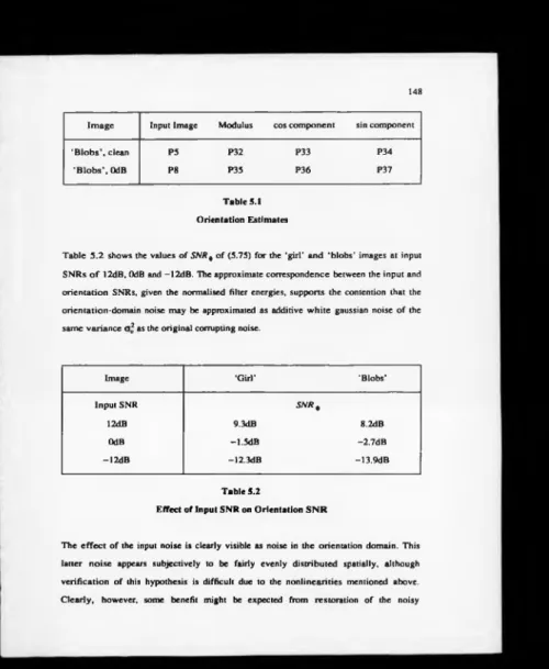
All photographic figures are prefixed with ‘P ’ (for exam ple figure P23), and are situated at the end o f the thesis. Other figures are indexed by c h a p te r (for example figures 5.1 to 5.4 in chapter 5) and are located at the end o f each chapter.

(28)

18

CHAPTER 2

QUADTREE STRUCTURE AND NEW IMAGE M ODEL

2.1 Motivation

As noted in Chapter 1, the minimum mean squared error (M M SE ) criterion provides a tractable basis for the design o f optimal estimation schemes. I t is a goal o f the present work that such MMSE optim ality be retained, but in a form o f estim ator (and underlying image model) which is better suited to the problem o f image restoration than the models

discussed in Chapter 1.

A noncausal model and estimator are sought on the grounds that:

(i) Causality is not an appropriate attribute for image m odels i f it is not mandated by ‘real-tim e’ considerations such as arise in on-line raster-scanned applications;

(ii) Noncausal estimators based on noncausal signal m o d els achieve lower m ean squared error than d o corresponding causal models for a giv en class o f signal. This results from the fact that the estimator is able to use ‘fu tu re ’ as well as ‘p ast’ input values and so has more data on which to base the estimate.

(29)

19

Another desirable property o f image models is nonstationarity. Natural images contain profound statistical nonstationarities such as lines and edges, an d a realistic image model should account for this fact.

A stationary image model under stationary degradation (blur o r noise) will give rise to a shift-invariant estim ator which necessarily performs the same operations at every point in the image. This is clearly less than ideal in the context o f natu ral images which tend to contain smooth regions with sharp edges, since a spatially-invariant restoration scheme which aims to smooth out noise is bound also to smooth salien t linear features in the image.

Such features are known additionally to be o f great im portance to the visual system. Much evidence now exists[9][54][55][82] for the presence in th e low er levels o f the visual system o f nerve cells (neurons) which function as linear feature (line and edge) detectors, implying that detection o f such features constitutes an early an d fundamental stage of visual perception. A s a consequence, image modelling and estim ation schemes w hich are based on stationary statistics are bound to produce visually unsatisfactory results.

(30)

20

tionally expensive since they generally involve the optimisation o f the estim ator at each point in the image.

This computational expense has led to the development o f ‘m u ltiple-m odel’ strategies which combine a fixed num ber o f stationary models in a spatially-variant manner, in order to achieve some degree o f spatial adaptivity without the need f o r the comprehen sive recalculation at every image pixel o f the model and its associated op tim al estimator.

The multiple-model approach o f Woods[152][157], for example, follow ing the original work o f Lebedev and Mirkin[83], uses five different stationary (M arkov random field) causal models and switches between them on the basis o f a controlling, higher-level model (a Markov chain) which governs the conditional probabilities o f the transitions (see also [59]).

The computational and memory requirements are still rather dem anding, since the method o f [152] involves running a large number (25) o f Kalman filters in parallel, each o f which must carry forward its own state information; in addition, th e selection o f the currently operative m odel requires the calculation and sorting o f the sam e num ber (25) o f the a posteriori probabilities o f each model, conditioned on the data, a t ea ch pixel.

Unfortunately, the parameters o f both the higher- and lower-level m o d els in [152] are estimated from uncorrupted versions o f the source images, noisy v ersio n s o f which are to be restored, and it is not clear how the system would perform given o n ly the noisy data as would probably be the case in any practical application.

(31)

21

the ‘w rong’ model has to continue for a finite period before it is possible reliably to detect that a change is required. The system o f [152] exhibits this ‘inertial’ tendency for the currently-selected model to persist for some time after it has ceased ad equately to represent the data.

Kashyap[72] has used another multiple-model approach, termed the ‘m ultivariate random field’, in which small segments (blocks) o f an image are assumed hom ogeneous and each m odelled by a stationary random field; the variation o f the model param eters from one block to the next is described by a higher-level (vector) random field.

W hilst multiple-model approaches have achieved better results than the u s e o f single m odels, the problems mentioned above restrict their effectiveness particularly in regions o f abrupt and pronounced nonstationarity such as edges, and this is precisely w here pro cessing adaptivity is m ost required. The use o f causal strategies is bound to le a d to poor results in edge regions, even in multiple-model schemes.

A m ore ‘continuously variable’ modelling approach was introduced by A b ram atic and Silverman[3], who defined a ‘signal-equivalent’ model which aims to incorp o rate the linear feature sensitivity o f the visual system into a modified image representation. The image is modelled essentially as a combination o f stationary lowpass and nonstationary highpass components, and the optimal (Wiener) filter for the lowpass c o m ponent is com bined in a spatially-variant manner with an identity operator such that less sm oothing is applied to the noisy image in edge regions.

(32)

the estimation operator. T h is leads to an estimation strategy which is both nonstationary and anisotropic, m atching m ore closely both the properties o f natural image features and the known m echanism s o f vision.

However, the further o n e m oves away from a purely stationary image estimation scheme toward ‘full’ nonstationarity (as opposed to the limited nonstationarity o f multiple-model approaches) and even anisotropy, the greater in general is the computational burden. In the present work, it is desired that ‘full’ nonstationarity be available, but that the associ ated computational o verheads be kept to the bare minimum.

Another property o f natural images which might profitably be incorporated in a more realistic image m odel is scale invariance (see section 1.5). The structure o f the natural world often looks sim ilar o v er a number o f different scales! 150]. (Consider, for example, the observation that in an electron micrograph o f a particle surface one sees ‘hills’, ‘val leys’ and so on). Edges in particular m ay exhibit some degree of fractal structure[87], and thus it w ould seem appropriate for the model to possess such properties.

Finally, the ‘end-user’ o f processed images is often the (human) visual system, and its fidelity criterion is very different from minimum mean squared errorfl0][27][88][124][129][132]. A s noted above and in Chapter 1, the visual system places m uch m ote em phasis on oriented features such as lines and edges.

(33)

23

Hence the fidelity criterion o f the visual system is at least nonstationaiy and anisotropic, and probably difficult to encapsulate in a mathematical form which both provides a com plete description o f its properties and admits a tractable form o f optimal estimator.

In the light o f the above, a choice is forced in the design process (see section 1.6). Either the MMSE criterion is abandoned in favour o f heuristic methods (such as the median filter[34]) or, if it is desired that the basis o f optimality be retained, the error criterion or equivalently the signal model m ust be modified to incorporate some o r all o f the desired characteristics.

In this work, it is desired that the M M SE criterion be retained as the basis for optimisa tion. What is sought is a noncausal, nonstationary image model giving rise to a noncausal, nonstationary but fast (i.e. computationally efficient) optimal estimator which is capable o f incorporating m odifications suggested by visual system properties.

2.2 Quadtree Structure and Applications

The quadtree[58][136] is the sim plest o f a class o f pyramidal data structures which have found increasing application in im age processing and computer vision work. Its introduc tion by Tanimoto and Pavlidis[136] in 1975 was the first attempt to provide a data struc ture matched to the ‘m ultiresolution’ representation o f images, which has become recog nised as valuable in a num ber o f application contexts.

(34)

24

structure resembles a square-based pyramid. It is common for each higher level to be of half the linear dimension (one quarter o f the area or number o f nodes) o f its predecessor. Note, however, that the term ‘quadtree’ specifically implies that each node is linked only with four nodes on the level below and with on e on the level above — a more general structure in which lateral and/or other vertical interactions occur is not a quadtree.

In image coding, the multiresolution approach offers the possibility o f separating in some sense those components o f an image which are o f different scales. Not only does this pro vide a substantial decorrelation o f the data, b u t it allows ‘coarse’ features to be encoded economically and transmitted before the finer detail. Such ‘progressive transmission’ techniques[73] build up what may be an adequate partial form o f the image at the receiver with minimal information transfer.

Wilson[148] has used a quadtree method fo r predictive image coding, where the d ata at a node is form ed by simple averaging over the fo u r nodes to which it is linked on the level below. Quantisation and transmission com m ences with the top level (a single node) and proceeds in a recursive m anner, with the difference between the value at a node and the quantised value at its parent being encoded. T h is scheme illustrates the general philoso phy o f pyram id coders and indeed o f the present work; the data structure permits the use o f sim ple predictive (DPCM) coding without constraining the coder to be causal in the image plane as is the case in conventional DPCM systems.

(35)

25

band be required. T he representation is invertible in that the original image may be recovered exactly (neglecting quantisation) from th e data in all o f the levels o f the pyramid.

Adelson e t al[4] have more recently discussed variants on the pyramid coder, including hexagonal and quincunx geometries and the use o f quadrature mirror filter (QMF) ker nels fo r the generation o f the pyramid. Good reconstruction quality at a respectable data compression ratio w as reported.

Cohen, Landy and Pavel[21] among others have applied quadtree coding to binary (car toon) images. Here the node value is a binary attribute, and a node is labelled with the attribute i f any o f the nodes to w hich it is linked on th e level below possesses it. The cod ing scheme is sim ilar to that o f W ilson mentioned above except for the binary nature of the data. Sparse cartoon images are particularly w ell suited to this type o f coding, since for m uch o f the im age there will be no activity and in such regions the coding procedure may term inate economically at a high level o f the quadtree.

Another m ajor application area is the field o f object/background or texture segmentation.

(36)

Rosen-26

feld[114], Hong and Shneier[50], and Hong, Shneier and Rosenfeld[51] among others. The latter work deals with edge extraction by the use o f edge d ata in such a pyramid rather than region interiors. Chen and Pavlidis[17] have used a pyram id data structure for their ‘split and m erge’ segmentation algorithm. Cohen and Cooper[20] use a modified quadtree for their hierarchical texture segmentation method, w hich is based on a M arko vian texture m odel. Peleg at al[l 12] have studied the properties o f textures in multiresolu tion representations from the viewpoint o f random fractals[87], by considering the rate of increase o f the area o f a texture surface as the measurement resolution increases.

Spann and Wilson[130] have developed a quadtree-based segmentation method. This first involves smoothing by forming the quadtree o f the image by averaging, and then classification at an upper level o f the quadtree using a ‘local cen troid’ clustering algo rithm! 147]. The classes thus obtained are propagated downward, with the positions o f the interclass boundaries being estimated at each level such that a t the image plane, the boundaries are only one o r two pixels wide. This work addresses explicidy the problem o f uncertainty[146][149], which lim its the performance o f m any signal and image pro cessing techniques in that it defines a bound on the degree to which global properties, such as statistical or frequency-domain parameters, and local spatial properties may simultaneously be effective. In segmentation, for example, the uncertainty principle dic tates that certainties in class membership and in position are incompatible and that a tradeoff must exist. The same principle limits the degree to w hich edges may be localised in the presence o f noise; this problem will be addressed in a subsequent chapter.

(37)

27

Ranade and Shneier[122] have used a multiresolution (quadtree) adaptive smoothing technique. A quadtree is formed by averaging, and the smoothing process seeks to preserve edges in the image by proceeding downward in the quadtree until a node is reached below which there is little activity in the image, and assigning to all nodes below it the average value at the given node. Active regions such as edges are therefore assigned an average computed over a small region. The method is, however, somewhat

a d hoc and m akes no claim o f optimality.

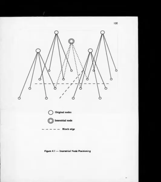
The properties o f pyramid generating kernels have been considered by M eer, Bauer and Rosenfeld[92] and more recently by Watson[142], Wilson and Spann[150], and Wilson and Calway[145]. These workers note that simple spatial averaging will lead in the absence o f explicit lowpass filtering to distortion caused by alias components! 120] induced by the reduction in sampling rate as the pyramid is ascended. This is undoubt edly true o f an y kernel which exhibits less than total (and unrealisable) attenuation at spatial frequencies above half o f the newly reduced sampling rate[142]. The introduction o f lowpass (‘anti-alias’) filtering involves a considerable computational overhead, how ever, and it will be shown in Chapter 4 that this precaution may in certain cases be unnecessary.

2.2.1 Q uadtree Sructure

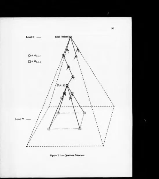
The quadtree is a pyramidal structure in which image data is represented on a number of different levels. A given level / consists o f (/i/X /i/) nodes (l , i , j) where

i , j , 0 £ i, j <, /i/ — 1 are the position coordinates o f the node within the level.

Each node (l , i , j) on level / is linked to four nodes ( / + on level /+ 1 , where

(38)

28

Level /+ 1 is conceptually below level /. The node ( l , i , j ) is known as the ‘father’ o f the four nodes (/+ 1 , f , f ) (its ‘children’). Level /+1 com prises (2 nt x 2nt ) = ( n /+1 x n /+1)

nodes.

Level 0 contains ju st one node, known as the ‘root’ o f the tree; this is the node (0,0,0). The bottom level is level Y and is o f the same dimension as the image data (in the present case n Y = 512 and Y = 9 ).

The structure is depicted in figure 2.1.

A data v alue at a node is denoted as, for example, S[ ¡ j or x tt ¡ j . T he term ‘for all i , j ’ will imply O S i , . / ¿ n ; - l i f the level index / is clear from the context.

2.2.2 Ancestor and D escendant Sets

For a given node ( /, / , j ) in the quadtree, two sets o f related nodes m ay be defined.

The ancest or set is defined as

A U J = [ ( k , p , q ) : 0 Z k * l ,

2 '-* p S I < 2l~ * ( p + 1) ,

2 '-» « S J c ï ' - ' l q + 1 ) ) , (2.1)

and the descendant set as

(39)

29

2 * - 'i S p < 2 * - '( i + 1) .

2 * -'y s , <2*-'U + l)) .

(2.2)

Note that (l , i t j ) e A l t i j and (l , i , j ) e D l i j. The ancestor and descendant sets are illustrated in figure 2.1.

The set o f all nodes in the quadtree may be denoted by

D0>o,o

•

The lowest comm on ancestor (LCA) o f two nodes ( /, i . j ) and ( k , p, q) is given by

L C A ( l , i , J ; k , p , q ) = ( r . m . n ) (2.3)

where

( r , m , n ) e ( A i , i j r \ A k p q )

and

( r + l , s , t ) 4 ( A i ' i j n A k ' P' q )

for any s, t . T he symbol r> denotes the intersection set.

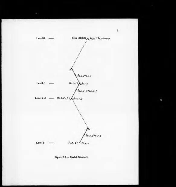
2.3 A New Im age Model

An image m odel, based on the quadtree structure, is defined as

(40)

30

f

.

where Wk,p.q has a gaussian probability density function (pdf) and

(2.5)

where bs t is the Kronecker delta function.

T he model characterises an image as being generated by a random process defined on the quadtree. The process operates ‘vertically’ dow n the tree starting at the root node (0,0,0)

This representation o f the model expresses a child node in terms only o f its father and a gaussian variable. The form o f the model is illustrated in figure 2.2.

T he fik.p.q arc the parameters o f the model and in general vary with p, q (i.e. with spa tial position on level k ). For the present, attention will be restricted to the spatially invariant form o f the model, where Pk.p. q ~ P* • The spatially variant model will be

and expresses the image as a sum o f gaussian random variables o f variance P 2

T he model o f (2.4) may be expressed in the recursive form

s i + i , r , f -

+ P/+i,r,/w/+i,r,/ *

(/+l,r,/)€D <>it>

0 £ / £ Y -1 , (2.6)

with initial condition

(41)

/

considered in Chapter 4.

31

2.4 Properties o f the Model

2.4.1 Noncausality

T he model (2.6) is a martingale [110] causal in the level index / . However, as a conse quence o f its vertical nature, there is no preferred causal direction in the horizontal (spa tial) plane and in the context o f the image (as generated at level Y o f the quadtree) the model is noncausal.

There is no tem poral order on the image pixels such as that imposed by raster scanning, which gives rise to spatially causal models and causal estimators such as the Kalman filter[69].

T he equation (2.6) may be considered to be a causal m inimum variance representation (M VR) [86] o r innovations representation [68] for s... and so the m odel retains the sim ple causal structure provided by these representations while not restricting the image

Sy,.,.

to be a causal signal.

2.4.2 Scale Invariance

D ata S i ' i j at a node (l , i , j) projects on to the image plane (level T ) at all pixels

(42)

32

Since the m odel o f (2.6) is clearly isomorphic at all levels, it generates features in the image-plane projection Sy p q at all scales. Thus the model may be seen to be scale-

invariant.

The values p / at higher (smaller / ) and lower (larger / ) levels o f the tree control the gen

eration o f larg er and smaller image features respectively. This relates in an obvious way to the notion o f scale invariance in natural images[150] (see section 1.5). Marr[91] com ments, indeed, that

‘The spatial organisation o f a surface’s reflectance function is often generated by a num ber o f different processes, each operating at a different scale.’

The m odel is formulated in such a way as to incorporate not only the basis of scale invariance, b u t also this notion o f ‘scale independence’.

There is also some relation to the fractal concepts o f Mandelbrot[87] which are based in notions o f scale invariance. The ‘partial’ images generated at different levels by this model bear comparison with random fractal functions, and sections — consisting o f the same num ber o f pixels — from different levels o f the tree would appear similarly ‘rough’ given sim ilar P parameters. A texture field as generated by the m odel might be character ised by its P parameters by analogy with the fractal-based texture description scheme of Peleg et al[ 112] mentioned in section 2.2.

(43)

33

2.4.3 Correlation Properties

The general correlation function for signals / ...and g...is defined as

I . J ' . k . P. « ) = • <2-*>

Then from (2.4) and (2.S), the following three correlation functions m ay be defined:

0 ) R - w ( ... : ... )

(2.9)

(H ) R s w (... ; ...)

R sw( l t i , j i r , m , n ) = E s i j j W r m n

- Z PkKw w i * ' P ' <r* r , m , n )

=

Z

$k& k.r& p.m& q.n

•

Thus

/?„»(/, i. j; r, m , n )

Pr , ( r , m , n ) e A i %ij ,

0 , (r , m , n ) 4 A i j j .

(2.10)

(44)

34

R „ ( l , i , j ; r , m , n) = Eslt

= Z

Z P

k ^ d ^ w k , p , q w d ,a ,b

( k . p . q ) ( d .a . b ) e A , ' , j • A r,m,a

= Z

Z PitPdSi.rfôpaS^/,

<*.#>.«) W.«.*)

eAl.,J € Ar tm,m

or

m £ P? (2.11)

( k . p . a ) e

Note that the expected energy E s f t i j increases monotonically w ith the level index / :

E * b . i - K m V . t . w . t . n

= P j + • •• + P? . (2.12)

It is possible following (2.11) to define a cum ulative correlation function

B ( l , i , j ; k , p , q) = £ R „ ( k , a , b ; k , p , q ) ,

( k . a . b )

k Z l . (2.13)

This function represents the sum o f the correlations between a node sk p q and all o f the descendants o f the node ( / , / , / ) which are on level k.

Now if ( k , p , q ) 4 D l t ¡ j then

(45)

35

0k , a , b ) e D l i ' j , (2.14)

and so

B ( l , l . j ; k , p . q ) - . (2.15)

Alternatively, i f ( k , p , q ) e D i i j then

B U . i . J - . k . p . q ) = 4‘ - ' / i „ ( i . i . J ; / . i . y ) + 4 * - '- 1p ? .1+ + ( tf (2.16)

or. by (2.12).

4 ) = 4 * - '( P 2 + ■ + P ? ) + 4 * - '- ‘P ? .,+ + (2.17)

It is also possible to define a one-dimensional average correlation as a function o f dis placement parallel to one o f the spatial coordinates on a level / :

T ( l , p ) “ TT Z R „ ( l . m . n ; l , m * p , n ) . (2.18) ™ (/. m, n)€D0.o.o :

(l,m + p,n)eD o.ofi

where W is the num ber of term s inside the summation.

Evaluation o f (2.18) yields

T ( t , p ) £

k=0 *=0

(2.19)

where n ( p ) is defined by

(46)

36

and n (0) = -1 .

T h e coefficient

o f p* in (2.19) is m onotonically nonincreasing with p.

By w ay o f example, the average correlation between tw o nodes on level 8 o f the quadtree at a separation o f 30 nodes is given by

T h e function T ( l , p) m ay be seen from (2.19) to be a strictly nonincreasing function o f

P-T ak in g the z transform o f T ( l , p ) in the variable p yields, assuming nonnegative definiteness o f T ( l, p), a spectral density function (SDF) as

(2.22)

an d that between nodes on level 5 at a separation o f 7 is given by

r<

5 ,

7 ) - do

2 + -if-P? +

■

(2.23)

(47)

37

$ ( « '“ ) l - 2 k- ‘p ]

1 -2

~‘p

J

cospco . (2.25)

2.4.3.2 L o n g -R ange Structure

Unlike m ost co m m o n image m odels such as the Markov random field (MRF) [153], the present model exhibits structure (i.e. correlation) over considerable distances in the image. This fo llo w s because any tw o image nodes with a given lowest common ancestor (LCA) have th e same correlation as any other tw o nodes with the same LCA. One may therefore sp eak o f image ‘blocks’ being correlated.

(48)

38

2.4.3.3 Dyadic Shift Invariance

The correlation function o f (2.11) is invariant to permutation o f the spatial positions of the descendants o f the n o d e s ( /, i , j ) or ( r , m , n ) within their respective descendant sets

DU j and Dr m n .

Such a permutation corresponds to a dyadic shift o f blocks within the image, and hence the image correlation fu n ctio n is dyadic shift invariant[5].

2.4.4 Analogy with Fractal Surfaces

If a level / o f the quadtree as generated by the model is visualised as a solid com posed of rectangular blocks, each w ith height s ^ i j (which may be negative) and base area 4 1

then as / increases, the surface o f this solid becomes increasingly subdivided an d its area also increases.

As / becomes arbitrarily large, and assuming nonzero values o f P/ , the surface area

increases without bound w hile its projection on the horizontal plane (the total base area) remains fixed.

(49)

39

Note that, like the area, the average energy o f a node o n the surface as given by (2.12) is unbounded as / —>«»>.

If, however, only a finite number o f the P; are nonzero then the surface has finite area

and a fractal dimension o f 2.

It seems likely that the interm ediate case, where Py - ♦ 0 as / -» , would give a fractal surface o f dimension between 2 an d 3, the exact value depending presum ably on how fast P/ approaches zero.

2.4.5 Range o f the Model

T he image generated by the m odel possesses a block structure, with blocks o f all scales superimposed. The parameters P/ determ ine the expected degree o f activity at each scale.

A few degenerate cases illustrate th e range o f the model.

• If P; = 0 for / > 0 , the m odel generates an image which consists o f a uniform gray

level.

• If pj = 0 for / < Y , the m o d el generates a gaussian white noise field o f variance

p f .

(50)

40

Thus the model represents the image as ( T + l ) superimposed ‘block white noise’ images, with scales ranging from the entire im age to single pixels, with varying weights. The similar but separate treatment o f different scales corresponds to the twin notions o f scale invariance and scale independence alluded to in section 2.4.2.

There is a correspondence with ‘p rogressive refinement’ or ‘progressive transmission’ algorithms, as applied to image coding[73], in that as the quadtree is descended the image becomes increasingly complicated with sm a lle r and smaller structure. The intermediate levels o f the quadtree resemble the block-structured images used by Harmon[45] in his work on the recognition o f faces.

2.5 Examples o f Model-Generated Images

Figures P I to P3 show examples o f im a g e s synthesised by the model o f (2.4) or (2.6). The upper photograph in each figure sh o w s level Y of the quadtree and the lower shows levels 0 (at the bottom) to Y —1.

In figure P I, the model parameters (3/ a re equal, P2 = 1 . In figure P2, p 2 = ( 3 /2 / and in figure P3, P 2 = ( 2 /3 / . The values o f P 2 for each level / in each figure are given in

table 2.1.

(51)

/

41

Figure PI P2 P3

0

? = > (3/2)' (2/3)'

L e v e l/ P?

1 1 1.500 0.6667

2 1 2.250 0.4444

3 1 3.375 0.2962

4 1 5.063 0.1975

5 1 7.594 0.1317

6 1 11.39 0.0878

7 I 17.09 0.0585

8 1 25.63 0.0390

9 1 38.44 0.0260

T a b l e 2 .1

V a lu e s o f p 2 f o r F i g u r e s P I — P 3

2.6 Comments on the Model-Generated Exam ples

The block structure o f the generated images is ap p aren t from figures P I to P3. The block edges coincide with boundaries in the quadtree. Since the same (pseudo-)random gen erator and seed (initial condition) were used fo r each o f the three figures, the wt>tj o f

(2.4) o r (2.6) are identical in each figure and th e differences between the figures are due solely to the values o f P/ employed.

If the P parameters were spatially variant, P = Pl , l , j • onc would expect the degree o f

(52)

42

Obviously, many natural images do not possess such sim p le geometric structure and an inexpensive method for reducing the blocking effect w ill b e introduced in C hapter 4.

However, natural images are often represented very p o orly by such models as the Mar kov random field, which tend to generate textures w ith structure at a particular scale which depends on the model order.

In the examples o f figures P I to P3, it is apparent that structure exists at all scales and hence, for the larger scales, over sizeable distances in th e image. In this sense the model captures an important property o f natural images (see sectio n s 1.5 and 2.4.2).

The ‘vertical’ causality o f the model may be seen by follow ing a feature from one of the upper quadtree levels (lower in the figures) through th e larger and successively more complicated images to level Y , the image plane.

2.7 Digital Filtering Interpretation of the Model

Figure 2.3 depicts the recursive form o f the model (2.6) a s a time-varying recursive digi tal filter. The time direction corresponds to the level in d ex / o f the quadtree. Neglecting the time-varying multiplier, the filter has a pole at z = 1 an d is thus m arginally stable.

2.8 Correlation Transforms

Only the one-dimensional case will be considered for the sake o f clarity.

(53)

43