The role of surface plasmons in metal enhanced chemiluminescence

M

’

A

P

The role of surface plasmons in

metal-enhanced chemiluminescence

Jesse Mak

February 7, 2014

G

Prof. Dr. Jennifer L. Herek

Prof. Dr. Ir. Alexander Brinkman

Dr. Christian Blum

Dr. Jord C. Prangsma

a_{Optical Sciences group,}b_{Quantum Transport in Matter group,}c_{Nanobiophysics group}

Optical Sciences group and Nanobiophysics group

Faculty of Science and Technology

AUTHOR Jesse Mak

jesse.mak@gmail.com

GRADUATION COMMITTEE Prof. Dr. Jennifer L. Hereka Prof. Dr. Ir. Alexander Brinkmanb Dr. Christian Blumc

Dr. Jord C. Prangsmaa,c

a_{Optical Sciences group,}b_{Quantum Transport in Matter group,}c_{Nanobiophysics group}

Optical Sciences group and Nanobiophysics group Faculty of Science and Technology

Contents

Acknowledgements 1

Abstract 2

1 Introduction 3

2 Chemiluminescence 6

2.1 Mechanism of chemiluminescence . . . 6

2.2 Efficiency of chemiluminescence . . . 7

3 Optical antennas 9 3.1 The complex dielectric function of metals . . . 10

3.2 Plasmonic resonances in quasi-static structures . . . 11

3.3 Plasmonic resonances in elongated structures . . . 13

4 Luminescence near optical antennas 15 4.1 Radiative and non-radiative decay near an antenna . . . 15

4.2 Model for enhancement . . . 16

4.3 Plasmon-enhanced chemiluminescence . . . 18

5 Experimental aspects 19 5.1 Antenna sample . . . 19

5.1.1 Design and fabrication . . . 19

5.1.2 Scanning electron microscope inspection . . . 21

5.1.3 Sample cleaning . . . 21

5.2 Dark field characterization setup . . . 22

5.2.1 Experimental setup . . . 22

5.2.2 Typical dark field spectrum . . . 22

5.3 Fluorescence microscope . . . 23

5.3.1 Experimental setup . . . 23

5.3.2 Typical gold luminescence spectrum . . . 24

5.3.3 Typical fluorescence time trace . . . 26

6 Results and discussion 27 6.1 Dark field scattering spectra . . . 27

6.2 Gold luminescence spectra . . . 29

6.4 Lucigenin fluorescence and chemiluminescence . . . 33

6.5 Methylene blue fluorescence . . . 36

6.5.1 Measured time traces . . . 36

6.5.2 Analysis using photon count histograms . . . 38

6.5.3 Comparison of different-sized antennas . . . 39

6.5.4 Control experiment using water . . . 40

7 Conclusion and outlook 43

References 45

Acknowledgements

First of all, I would like to thank Jord, my daily supervisor, for his devotion to the project, his insightful explanations, and original ideas. It was a pleasure to work with you Jord. I would also like to thank Dirk Jan, who helped with experiments and provided valuable feedback on the project.

Furthermore, my thanks go out to Stefan for synthesizing gold flakes, to Frans for his excel-lent work with the focused ion beam, and to Ron Gill for providing me with an interesting fluorescent dye. I also thank Tom and Simon for their motivating and calming support. I par-ticularly thank Simon for his advice on presenting my work.

I thank Jeroen for additional technical support and Karen and Carin for administrative sup-port. In fact, I am grateful to everyone in the Optical Sciences and Nanobiophysics groups for their contributions to the project and for the great social atmosphere.

I would like to thank Jennifer Herek for motivating and supporting me throughout the MSc programme. I especially thank her for arranging an amazing internship in Boulder. Next, I would like to thank my friends for the great time in Enschede. Special thanks to Sean, Luuk, Murat, and Roza, to student fraternity Πίθηκος ἁμάρτανοι, and to student house Da Bunch.

Finally, I am very grateful to Franziska and my family for their support.

Abstract

Chemiluminescence is used in many analysis methods as a sensitive reporter of the presence of biological materials. In a chemiluminescent process, a chemical reaction involving the sub-stance of interest leads to a reaction product in the excited state. This excited state can de-cay by the emission of photons. However, the quantum efficiency of this process is often low due to a multitude of non-radiative decay paths. Enhancing the radiative decay of the excited state is therefore of wide interest. Several studies have been performed to investigate the use of plasmons for this [1] however, none of these studies made use of plasmonic systems with well-characterized resonances.

We study lucigenin chemiluminescence and methylene blue fluorescence near different-sized optical antennas. The plasmon resonances were characterized using 1) dark-field scatter-ing spectroscopy and 2) spectroscopy of the intrinsic luminescence of the antenna material (gold). We observe an approximately linear relation between the resonance wavelength and antenna length, which is in good agreement with a Fabry-Perot resonator model for cylindri-cal antennas [2].

Lucigenin chemiluminescence has two major components that emit light: 1) N-methyl acridone, and 2) the lucigenin itself, excited by N-methyl acridone through Förster resonance energy transfer. We first study the emission of the second component, with excitation by light. Fol-lowing this, we study the complete chemiluminescent system. We show that the antennas in factdarkenthe emission, and explore several explanations.

The final part of the thesis presents a controlled study on the distance dependent enhance-ment of a fluorophore near an antenna. We observe fluorescence time traces with strong peaks whenever an emitter is in a favorable location with respect to the antenna, where en-hancement occurs. Most intensity enen-hancement is observed for a 70x110 nm antenna, with an enhancement factor of ~4.

1 Introduction

Sensitive detection of molecules is of central importance for a number of fields, such as phar-macology, bioscience, and environmental science [3]. An established method to detect molecules is to involve them in chemical reactions that produce light. This type of light emission is called chemiluminescence. It is routinely used as a reporter for molecules in clinical tests on,e.g., fer-tility, anemia, cancer, or infectious diseases [4]. In bioscience, it is used to mark the location of biological macromolecules (DNA, RNA, proteins) that have been sorted using membrane filters [4]. Other applications include the detection of environmental pollutants [3] and the detection of blood in crime scene investigation [5].

Chemiluminescence-based techniques have advantages over other detection techniques. In contrast to fluorescence-based detection, no external light source is required. Therefore, problems such as light scattering, source fluctuations, and high backgrounds due to unselec-tive excitation are absent [6]. Furthermore, chemiluminescence reagents are considered to be less hazardous than alternative techniques using radioactive isotopes for tracing chemi-cals [6].

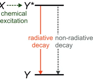
In a chemiluminescent process a chemical reaction involving the substance of interest leads to a reaction product in an electronically excited state (see Fig. 1.1). This excited state can decay by the emission of photons. However, the efficiency of this process is often low due to a multitude of non-radiative decay pathways. Enhancing the radiative decay of the excited state is therefore of wide interest.

Y

Y*

X

chemical excitation

radiative decay

non-radiative decay

Figure 1.1: Simplified energy level diagram for chemiluminescence. A chemical reaction involving

Xleads to a reaction product in the excited state (Y∗). The excited state can make a transition to the

ground state (Y) with the emission of a photon (radiative decay), but it can also return to the ground

state by a radiationless process (non-radiative decay).

plas-monic nano-antennas [7]. Near an optical antenna, the radiative rate can increase because there are more pathways that lead to the radiation of a photon to the far-field. This is one of the reasons why fluorescence shows an enhanced intensity near metal plasmonic nanos-tructures [8, 9].

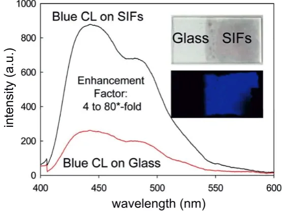
Several groups also report an enhancedchemiluminescenceintensity near metal plasmonic structures [1, 10, 11]. An example of these findings is shown in Fig. 1.2 [1]. We note that none of the studies made use of plasmonic systems with well-characterized resonances. As many chemiluminescent reactions require a catalyst [6], the metal may also catalyze (i.e. speed up) the reaction. In that case, the photons would be emitted within a shorter time-window, leading to a higher chemiluminescence intensity. Therefore, it is debatable whether there is enough evidence to ascribe the enhancement to plasmons.

wavelength (nm)

intensity (a.u.)

Figure 1.2: Enhanced chemiluminescence (CL) on silver island films (SIFs). The graph shows chemi-luminescence spectra on silver island films (black curve) and on glass (red curve). The insets show photographs of a glass microscope slide with silver island films (top) and the chemiluminescent mix-ture placed in between two slides (bottom). From Aslan and Geddes [1].

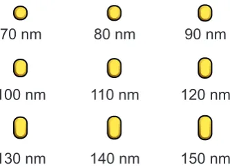
The aim of this research is to find evidence whether enhanced chemiluminescence can be ascribed to a plasmonic effect, a catalytic effect, or a combination of these. In contrast to earlier work, we aim to study chemiluminescence near a plasmonic system where the ge-ometry and optical properties are well characterized. For this reason, we designed an array gold antennas with well-defined lengths (Fig. 1.3). Such antennas have resonant plasmon modes at different wavelengths [2], and will only enhance emission of light with a similar wavelength. By comparing the chemiluminescence intensity near each antenna, we hope to find out whether enhanced chemiluminescence is a resonant plasmonic effect.

70 nm

150 nm

80 nm 90 nm

120 nm 110 nm

100 nm

130 nm 140 nm

Figure 1.3: Lay-out of the plasmonic nanostuctures. Nine nanorods with different lengths. Such structures have resonant plasmon modes at different, well-defined wavelengths.

by two independent methods using (1) dark field scattering spectroscopy and (2) spectroscopy of the intrinsic luminescence of the gold. Having characterized the plasmon modes, it was investigated whether the antennas enhance the chemiluminescence of lucigenin and hydro-gen peroxide. In these experiments, no enhancement is observed. It was realized that for enhancement to occur, strict conditions must be met. For instance, the level of enhancement strongly depends on the emitter’s location with respect to the antenna.

2 Chemiluminescence

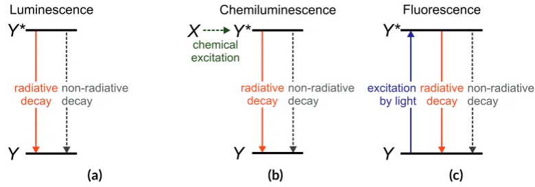
Luminescence is a term used for the emission of light, which occurs when a quantum system (f.i. an atom or molecule) makes a jump between two states with different energies [6, 12]. The various types of luminescence differ by their mechanism to obtain the high energy state. For fluorescence, the energy is delivered by electromagnetic radiation (see Fig. 2.1c). For chemiluminescence, it is delivered by a chemical reaction (see Fig. 2.1b). The current section mainly describes chemiluminescence. For a review on fluorescence, the reader is referred to literature [13]. Section 2.1 describes the mechanism behind chemiluminescence. To il-lustrate the mechanism, the reader is introduced to the chemiluminescence reaction of luci-genin, which is used in this thesis. Section 2.2 describes the efficiency of chemiluminescence.

Y

Y*

Y

Y*

X

Y

Y*

Figure 2.1: Simplified energy level diagrams for (a) luminescence in general, (b) chemiluminescence, and (c) fluorescence. Y is the ground state andY∗the excited state. In (b), the excited state is pro-duced by a chemical reaction. In (c), it is formed as the molecule absorbs electromagnetic radiation.

2.1 Mechanism of chemiluminescence

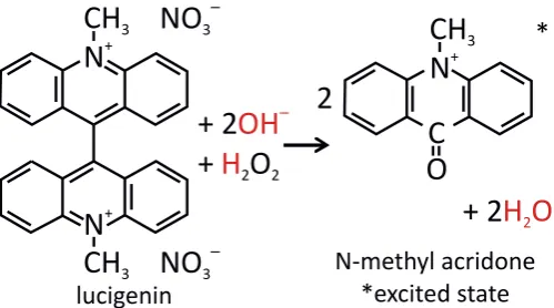
In a chemiluminescent process, a chemical reaction leads to a reaction product formed in an electronically excited state. Light is emitted when the molecule makes a transition to its ground state. To illustrate this, let us consider the chemiluminescent reaction of lucigenin and hydrogen peroxide (H2O2) used in this thesis. As shown in Fig. 2.2., lucigenin reacts with hydrogen peroxide to form N-methyl acridone (NMA) in the excited state. NMA can decay to its ground state with the emission of blue light. A base,f.i. sodium hydroxide (NaOH), is necessary to provide hydroxyl ions (OH-_).

+ 2

OH

+

H

O

+ 2

H O

*

2

CH

N

NO

N

CH

NO

CH

N

C

O

Figure 2.2: Reaction mechanism for the chemiluminescence of lucigenin.

can transfer its energy to the lucigenin. Lucigenin emits green light, so the observed color will change from blue to green.

In many chemiluminescent reactions a catalyst can be used to speed up the reaction. Cat-alysts are not consumed by the reaction. They provide a mechanism by which the reaction can occur that has a lower activation energy. Since the reaction rate depends exponentially on the activation energy, a slightly lower activation barrier can lead to a significant increase in reaction rate [14]. Since the chemiluminescence of luminol was first reported by Albrecht in 1928, several catalysts have been investigated, including metal ions and enzymes [15]. In 2005, Zhanget al. reported the use of gold nanoparticles to catalyze the reaction between luminol and hydrogen peroxide.

2.2 Efficiency of chemiluminescence

Chemiluminescence and fluorescence are both limited in efficiency because excited molecules can lose their energy through radiationless processes (e.g. internal conversion, intersystem crossing). Therefore, each excited molecule has a chance to decay radiativelyornon-radiatively. These competing effects are usually described with decay rates. An initial population of ex-cited molecules will decay radiatively at rateΓ_radand non-radiatively at rateΓ_nrad. The total

decay rate is given by

Γ_tot= Γ_rad+ Γ_nrad (2.1)

For a single excited molecule, the probability for radiative decay to occur is

Φ_q = Γrad

Γtot (2.2)

This expression is known as the quantum yield of the emitter. In Chapter 4, an explicit ex-pression forΓ_totwill be given. It will be shown that in the presence of an antenna, the balance

Whereas the efficiency of a fluorescent process is usually assessed with the quantum yield, chemiluminescent processes are characterized by a different term: the chemiluminescence yield. This is the fraction of target molecules (to be detected) that eventually cause the emis-sion of a photon: [16]

Φ = ΦrΦeΦq (2.3)

withΦ_rthe fraction of target molecules that undergo a reaction,Φ_ethe number of excited

molecules formed per reaction, andΦqthe quantum yield of the excited product as defined in Eq. 2.2. In case of indirect chemiluminescence, the chemiluminescence yield is defined differently:

Φ = ΦrΦeΦtΦq (2.4)

whereΦ_tis the efficiency of the energy transfer, andΦ_qis the intrinsic quantum yield of the

3 Optical antennas

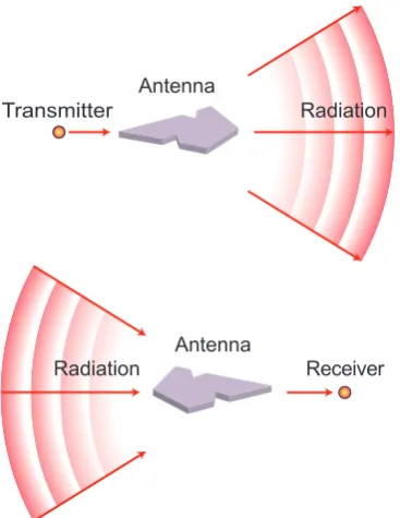
Antennas optimize the energy transfer between a localized source or receiver and the free-radiation field [17], as is shown in Fig. 3.1. This concept is widely used for radio- and mi-crowaves, but it can be extended to the optical regime. The sources and receivers then be-come nano-scale objects, such as atoms and molecules. Optical antennas are usually based on metal nanostructures, which can confine fields beyond the diffraction limit. To under-stand their working, one needs to underunder-stand the optical properties of metals, which can be described with a frequency-dependent dielectric function (Section 3.1). Light with the right frequency can drive the free electron gas of a metal nanostructure into resonant os-cillations. Resonant effects are most easily explained when the structure is much smaller than the wavelength of the light. This is known as thequasi-staticapproximation. Section 3.2 discusses resonant properties of a quasi-static sphere, such as enhanced scattering and ab-sorption. Elongated structures require a different treatment, as is discussed in Section 3.3. In particular, it is shown that for elongated structures, the resonance wavelength becomes size-dependent.

Transmitter

Antenna

Radiation

Receiver Antenna

Radiation

3.1 The complex dielectric function of metals

The optical properties of metals can be described using a frequency-dependent complex di-electric function(ω). This function enters Maxwell’s equations through the relation [18]

D=(ω)E (3.1)

An approximate expression for(ω)can be found using a Drude model, as is described in

several texts, such as [18]. The result is

Drude(ω) = 1− ωp 2

ω2_+iΓω (3.2)

whereΓis a damping constant andωpis the plasma frequency, a natural frequency at which the electrons tend to oscillate [19]. The plasma frequency is given byωp =

p

ne2_/(m

e0)

withn,eandmethe density, charge, and effective mass of the free electrons.

For gold, this model gives accurate results in the infrared regime, but in the visible regime in-terband transitionsshould also be considered. In such a transition, a high-energy photon pro-motes an electron to the conduction band of the metal [18]. This can be pictured classically as oscillations of the bound electrons, induced by electromagnetic radiation. The contribu-tion of a single interband transicontribu-tion is given by

Interband(ω) = 1 +

˜ ωp2

(ω02−ω2)−iγω (3.3)

whereωp˜ is the plasma frequency for bound electrons,γ is a damping constant, andω0 = p

α/m, withαthe spring constant for the potential that keeps the electrons in place, andm the effective mass of the bound electrons.

One can model experimental data for(ω)by adding contributions from the free-electrons

(Eq. 3.3) and a single interband transition (Eq. 3.2). Fig. 3.2 shows a comparison with experi-mental data from Johnson and Christy for gold [20]. An offset∞ = 6has been added to Eq. 3.3 to take into account all other interband transitions.

It is important to note from Fig. 3.2 that the real part ofis negative. For this reason, the refractive indexn=√will have a strong imaginary part. Therefore, electromagnetic fields can only penetrate the metal to a small extent. The length that the field penetrates is called theskin depth. Fig. 3.2 shows that as the wavelength increases,Re()becomes more

nega-tive. For radio waves (~1 cm - 1 km), the skin depth is therefore negligible compared to the dimensions of an antenna. For light waves (~400 - 800 nm), however,Re()is less negative.

0

5

10

Im(

ε

)

experimental data

_model

300

400

500

600

700

800

900

1000

−40

−20

0

wavelength (nm)

Re(

ε

)

Figure 3.2: Experimental values [20] and model [18] for the dielectric function of gold. The model takes into account the contribution of free-electrons (Eq. 3.3) and one interband transition (Eq. 3.2).

An offset∞ = 6has been added to Eq. 3.3 to take into account all other interband transitions. The

values used areωp = 13.8·1015s−1,Γ = 1.075·1014s−1,ω˜p = 45·1014s−1,γ = 9·1014s−1, and

ω0= 2πc/λ, withλ= 450 nm.

3.2 Plasmonic resonances in quasi-static structures

When the electric field of a light wave penetrates a metal nanostructure, it drives the free electrons into a collective oscillation called asurface plasmon(SP) [22]. At certain frequen-cies, the oscillation is resonantly driven. Resonant effects in metal nanostructures are most easily explained for structures that are much smaller than the wavelength. In that case, the quasi-static approximationcan be used. In this approximation, the applied field is considered to be uniform over the entire shape of the structure. It is only valid when the structure is smaller than the skin depth of the metal. In quasi-static structures, resonance effects can be found by solving for the electrostatic potential [22].

As an example, let us consider a metal sphere with dielectric function(ω)in vacuum in a

uniform field [18, 23, 24], which points in thexdirection. The field will push positive charge to the "right" surface of the sphere, leaving a negative charge on the "left" surface [24]. By first solving for the electrostatic potential, one can obtain expressions for the fields in and outside the sphere:

Ein =E0

3

+ 2(cosθnr−sinθnθ) (3.4)

Eout=E0(cosθnr−sinθnθ) + α 4π0r3

E0(2cosθnr+ sinθnθ) (3.5)

withαgiven by

α= 4π0a3 −1

Eq. 3.4 and 3.5 use spherical coordinates, withrthe radial distance,θthe polar angle, andn_r

andnθthe corresponding unit vectors.

It should be noted that the second term in Eq. 3.5 is identical to the field of a dipole located at the center of the sphere. The dipole moment is given byp =αE. It is important to study

the form ofα(Eq. 3.6). Whenever|+ 2|has a minimum, resonant behavior occurs. One can distinguish three resonance effects:

1. Enhanced local field. The physical field near the sphere can be obtained by taking the real parts of Eq. 3.4 and 3.5. Fig. 3.3 shows the field distribution for a gold sphere at resonance (532 nm). Near the left and right surface, the field is resonantly enhanced. This can be seen from Eq. 3.5 by noting that, when taking the real part,αchanges to Re(α). At resonance,Re(α)is very large, and therefore, so isRe(Eout).

−2

0

2

−2

−1

0

1

2

x/a

y/a

|Re(

E

/

E

)|

0

1

2

3

4

Figure 3.3: Field distribution near a gold sphere of radiusaat the resonance wavelength (532 nm).

Based on Eq. 3.4 and 3.5.=−4.60 + 2.44i, in accordance to data from Johnson and Christy [20].

2. Enhanced scattering. Suppose the particle is illuminated by a plane wave, with a time-varying electric field. The induced dipole moment will also vary in time. The radiation of this dipole leads to scattering of the plane wave. For the scattering cross section one can derive

Csca = k

4

6π|α|

2 _(3.7)

withkthe wavevector of the plane wave. At resonance,|α|is very large, so there will be enhanced scattering.

3. Enhanced absorption. Similar to the scattering cross section, one can define an absorp-tion cross secabsorp-tion:

Cabs =kIm(α) (3.8)

It should be noted that, for quasi-static structures, resonances are independent of particle size.

3.3 Plasmonic resonances in elongated structures

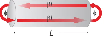
For elongated, rod-like particles, the applied field will differ in phase across the shape of the particle. In that case, the quasi-static approximation breaks down. The fields now create propagatingSPs that reflect at the antenna ends, forming a Fabry-Perot resonator (Fig. 3.4). For a detailed treatment of propagating SPs, the reader is referred to [18]. Here, it is impor-tant to note that

1. The SP has a propagation constantγ =β+αi, whereβdetermines the SP wavelength (λSP = 2π/β), andαaccounts for damping of the SP.

2. The SP penetrates into the surrounding medium. This leads to an additional phaseΦ

that is picked up upon reflection at the antenna ends.

This description is summarized in Fig. 3.4. The figure shows the phase contributions that the SP acquires as it travels back and forth a cylindrical rod. The condition for a Fabry-Perot resonance is [25]:

βLres+ Φ =nπ (3.9)

withLresthe resonance length of the rod andnthe order of the resonance (n= 1, 2, ...). The resonance length of the first order is then

Lres =π/β−Φ/β (3.10)

From a similar model by Novotny [2], we note that the second term can be approximated by

2R, whereRis the radius of the rod. One then obtains

Lres=π/β−2R (3.11)

f

L

b

L

b

L

f

Figure 3.4: Schematic picture of an SP propagating back and forth a cylindrical rod. Between the

two ends, the SP acquires a phaseβL. At each reflection, it picks up an additional phaseΦ. Image

As mentioned above,βis the real part of the propagation constantγ. To determineγ, it is necessary to calculate the modes of an infinite cylindrical waveguide. TheT M0 modes are solutions to the equation [2, 26]

(λ) κ1R

J1(κ1R) J0(κ1R)

− s κ2R

H1(1)(κ2R)

H0(1)(κ2R)

= 0 (3.12)

withκ1 = k0 p

(λ)−(k0/γ)2, andκ2 = k0 p

s−(k0/γ)2.1. Here,(λ)is the dielectric func-tion of the metal,sis the dielectric constant of the surrounding medium, andRis the radius of the cylinder. Furthermore,JnareHn(1)are Bessel and Hankel functions of the first kind.

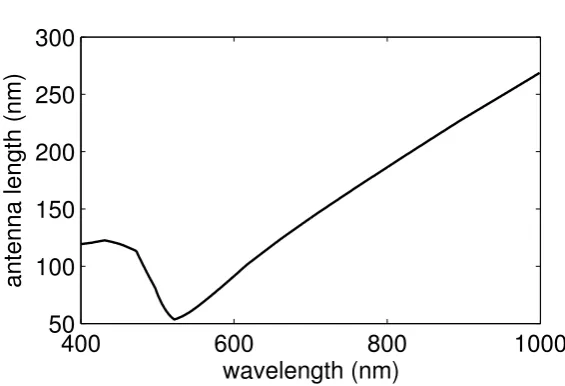
Fig. 3.5 shows how the resonance length depends on the free-space wavelength. The curve was calculated using Eq. 3.11, whereβ = Re(γ)was obtained by solving Eq. 3.12

numer-ically using a minimization algorithm2_{. Traditional antennas have a length that is half the} free-space wavelength. As the figure shows, optical antennas have a length that is a factor 2-5 shorter. In many texts, it is said that the antenna does not respond to the free-space wave-length, but to a shortereffective wavelength[2]. The relation between the antenna length and the effective wavelength is

Lres=λef f/2 (3.13)

400

600

800

1000

50

100

150

200

250

300

wavelength (nm)

antenna length (nm)

Figure 3.5: Resonant lengths for gold rods with radiusR = 20 nm, as a function of the free-space

wavelength. The curve was calculated using Eq. 3.11, whereβ = Re(γ)was obtained numerically

using Eq. 3.12. Experimental values forwere used [20]. The curve is closely related to the effective

wavelength curve from Novotny [2], according to Eq. 3.13.

1_{When taking the square root in these expressions, one finds two values. Forκ2, the value with positive} imag-inary part must be taken [26].

2_{Although there are approximate expressions to calculateL}

4 Luminescence near optical antennas

Many studies show enhanced fluorescence near metal nanoparticles [8, 9]. The enhance-ment is based on two factors. On the one hand, there is enhancedexcitationdue to the strong electric field near the antenna (see Section 3.2), which leads to a higher absorption rate of the fluorophore. On the other hand, as will be explained, there can be enhancedemissiondue to the optimized nanophotonic environment. In case of chemiluminescence, there is chemi-calrather than optical excitation (see Section 2.1). Therefore, enhanced excitation does not play a role, and will not be discussed. Instead, the current section describes enhanced emis-sion. Section 4.1 shows how the presence of an antenna can change the balance between radiative and non-radiative decay. It will turn out that antennas either increase or decrease the quantum yield. Section 4.2 presents a model for this behavior. This chapter ends with a literature overview on enhanced chemiluminescence (4.3).

4.1 Radiative and non-radiative decay near an antenna

Thetotaldecay rate of a quantum emitter in a dissipative environment can be determined usingFermi’s golden rule, giving [7, 21]:

Γ_tot(ω,r,e_d) = πd

2_ω

~0

N(ω,r,e_d) (4.1)

withωthe emission frequency,rthe position of the dipole,e_da unit vector indicating the

dipole orientation, anddthe modulus of the matrix element for the transition.N(ω,r,e_d)is

thelocal density of optical states(LDOS). Eq. 4.1 can be decomposed into two parts. One part accounts for the intrinsic quantum properties of the source through the transition matrix elementd. The other part accounts for the environment of the emitter through the LDOS.

By changing an emitter’s environment, one can increase the LDOS and thereby, through Eq. 4.1, the total decay rate. The presence of an antenna leads to a higher LDOS because pho-tons can be emitted through the modes of the antenna. However, some of these phopho-tons are lost because they excite higher order non-radiative modes. This means that the antenna not only increases the radiative decay rate, but also the non-radiative rate. For enhancement in intensity to occur, the increase of the radiative decay rate needs to behigher.

One can establish a classical analogue by noting that the LDOS can be expressed as

N(ω,r,e_d) = 6ω πc2(ed

T _·Im(

G(r,r, ω)·ed) (4.2)

of a dipole to the local environment. In Eq. 4.2,Gis evaluated at the location of the emit-ter itself. This reveals the fact that the decay happens in response to the emitemit-ter’s own field. When placed near an antenna, a classical dipole will experience a driving force from its own secondary field - the field scattered from the antenna and arriving back at the dipole’s po-sition. On the one hand, the dipole’s power may increase, due to constructive interference with the secondary field. On the other hand, the dipole’s power will be decreased due to absorption by the antenna.

4.2 Model for enhancement

The previous section showed how an antenna can increase both the radiative and non-radiative decay rate of an emitter. Whether intensity enhancement occurs, depends on the balance between the two. The current section presents a model for this behavior. The model is based on a dipole emitter near a spherical antenna [21, 27] like the one in Section 3.2, in air. The intrinsic quantum yield of the emitter is denoted as

Φ0_q = Γ

0 rad Γ0

rad+ Γ0nrad

(4.3)

In the presence of the sphere, there will be a new quantum yield:

Φ_q = Γrad

Γ_rad+ Γ_nrad (4.4)

However, as explained in Section 4.1, the antenna introduces a new loss channel, due to non-radiative energy transfer to the antenna. Therefore, the non-non-radiative decay rate is split in two:

Γ_nrad = Γ_abs+ Γ0_nrad (4.5)

Combining Eq. 4.3, 4.4, and 4.5, one obtains

Φq=

Γrad/Γ0_rad

Γ_rad/Γ0_rad+ Γ_abs/Γ0_rad+ [1−Φ0

q]/Φ0q

(4.6)

To determineΦ_q, one needs to find expressions forΓ_rad/Γ0

radandΓabs/Γ0rad. For a derivation, the reader is referred to [21, 27]. Here, we will only state the expressions and note their consequences.

Γrad Γ0_rad =

1 + 2 ˜α a 3

(a+z)3 2 (4.7) Γabs Γ0_rad =

3 4Im

₋₁ + 1

₁

(kz)3 (4.8)

the polarizibility of the sphere as in Eq. 3.6 (Section 3.2).

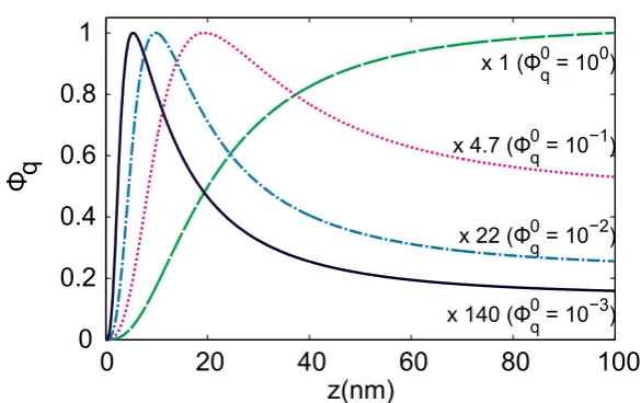
0 20 40 60 80 100

0 0.2 0.4 0.6 0.8 1

x 1 (Φ q 0

= 100)

x 4.7 (Φ q 0

= 10−1₎

x 22 (Φ q 0

= 10−2₎

x 140 (Φ q 0

= 10−3₎

z(nm)

Φ q

Figure 4.1: Quantum yield of an emitter near a gold sphere, as a function of their separation dis-tance, for emitters with different intrinsic quantum yields (Φ0

q). The sphere has radiusa = 40 nm,

and=−9.30 + 1.54, in accordance to data from [20] at600 nm. The curves are scaled to the same

maximum value. Based on the model by Bharawaj and Novotny [21, 27].

Using Eq. 4.7, 4.8, and 4.6, one can calculate the quantum yield. Fig. 4.1 shows the result for a gold sphere with a radius of 40 nm. The figure shows that when the intrinsic quantum yieldΦ0

q = 1, the antenna can only reduce the quantum yield. Furthermore, whether en-hancement occurs strongly depends on the distancez. For too large distances, there is no interaction between the emitter and the antenna, and the quantum yield is unchanged: i.e.

Φ_q = Φ0_q. For too small distances, energy dissipation dominates, and the quantum yield

de-creases:Φq<Φ0q.

Finally, it should be noted that the highest enhancement does not occur at the plasmon res-onance frequency. In fact, it occurs at a frequency that is shifted to the red part of the spec-trum. This can be explained by studying the resonances of Eq. 4.7 and 4.8. Eq. 4.7, which characterizes radiative decay, has a resonance governed by the denominator ofα(+ 2).

This is the familiar plasmon resonance (see Section 3.2). Eq. 4.8, which characterizes absorp-tion, has a different resonance, governed by+1. Although there is increased emission at the

4.3 Plasmon-enhanced chemiluminescence

5 Experimental aspects

To be able to study chemiluminescence in a system with well-defined resonances, an array of nanostructures was developed. Section 5.1 presents the design of these structures and ex-plains how they were fabricated. Based on scanning electron microscope (SEM) images, the quality of the fabricated structures is discussed. The experiments in this thesis were done using two experimental setups: a dark field setup and a fluorescence microscope. These are described in Sections 5.2 and 5.3.

5.1 Antenna sample

5.1.1 Design and fabrication

To compare the behavior of antennas with different resonances, 3x3 array of gold nanorods was designed (Fig. 5.1). While the antennas have the same width and depth (~70 nm and ~30 nm, respectively), their length increases (~70-150 nm). The structures were fabricated by focused ion beam (FIB) milling in a gold flake. To achieve this, single crystalline gold flakes were chemically synthesized and cast onto a glass cover slip (1x1 inch,no. 1.5). As a scanning electron microscope (SEM) was used for inspection, the flake samples were coated with a thin conducting layer (gold for one sample and gold-palladium for another; see below). This layer is necessary because glass substrates tend to charge during SEM-inspection, leading to distorted images. Finally, the antenna array was formed by FIB milling in one of the flakes.

70 nm

150 nm

80 nm 90 nm

120 nm 110 nm

100 nm

130 nm 140 nm

Figure 5.1: Design of the plasmonic nanostuctures. Nano-antennas with different lengths (~70-150 nm), but the same width (~70 nm) and depth (~30 nm).

The experiments in this thesis were done using two samples1_{. These will be referred to as} Sample 1 and Sample 2. Although the samples have the same design, there were some ences in the fabrication procedure. For one, the gold flakes were synthesized using a differ-ent recipe. The flake used for Sample 1 was relatively thick (~63 nm) and had to be thinned

2.5 µm

(a)Sample 1

2.5 µm

(b)Sample 2

down significantly to obtain an antenna depth of~30 nm. The flake for Sample 2 was ~42 nm thick, which required less thinning. Furthermore, a different conducting layer was used for each sample: a 10 nm gold layer for Sample 1, and a 5 nm gold-palladium layer for Sample 2.

5.1.2 Scanning electron microscope inspection

The quality of the structures will now be judged using scanning electron microscope (SEM) images of Sample 1 and Sample 2 (Fig. 5.2a and 5.2b). Some parts of the SEM images are brighter than others,e.g. the bright area in the north-east corner of Fig. 5.2a. This is as-cribed to charging of the glass substrate. We note that in both images, the nine antennas can be clearly distinguished. The distance between them is 2.5µm, which is considered to be large enough to avoid interaction between the antennas. Looking at the shapes of the nine antennas, it can be seen that the width stays approximately constant, while length gradually increases, as was intended in the design. For instance, the antenna in the upper-left corner is roughly square, while the antenna in the bottom-right corner is elongated. The area be-tween the antennas seems to be fairly flat, except for some graininess. It is expected that this graininess was caused while milling into the glass.

5.1.3 Sample cleaning

5.2 Dark field characterization setup

5.2.1 Experimental setup

EMCCD

Super-continuum laser

Mono-chromator

Figure 5.3: Schematic overview of the dark field characterization setup.

A common way to characterize the plasmon modes of a nanostructure is to illuminate it with a plane-wave and study the scattered far-field [28]. To characterize multiple structures, it is usually required to illuminate them one by one. However, the Optical Sciences group has developed a method to study many structures in parallel. The experimental setup is based on a dark field configuration, as shown in Fig. 5.3. In this geometry, the transmitted and re-flected beams are rejected by angular separation, so that only scattered light is collected. In our method, the samples are illuminated using a spectrally filtered white light continuum laser (Fianium SC400-4; 4 W; 40 MHz repetition rate). A single wavelength is selected using a monochromator (Acton SP2150i). A 50x50µm2area (potentially containing 400 separate

nanostructures) is then imaged on an EMCCD (Andor iXon3 897) for many different wave-lengths (400-1000 nm). To compensate for chromatic aberration, the sample is moved using a computer-controlled stage following a fitted curve.

5.2.2 Typical dark field spectrum

500 1000 1500 2000

counts _{in 0.5 s}

670 nm 710 nm 740 nm 790 nm

500 600 700 800 900 1000

0 0.5 1

intensity

(normalized)

wavelength (nm)

Figure 5.4: Procedure to obtain individual antenna spectra from the dark field images.

400 500 600 700 800 900 1000

0 0.5 1

wavelength (nm) sensitivity _(normalized)

Figure 5.5: Spectral sensitivity of the dark field setup.

It should be noted that Fig. 5.4 shows negative counts above 900 nm. The reason is that at a few wavelengths, the subtraction of the background led to a small negative number. This negative number was then multiplied by a large number to correct for the low system re-sponse function above 900 nm.

5.3 Fluorescence microscope

5.3.1 Experimental setup

an-AOTF

filter

filter

antenna sample

excitation

emission

synchronization

Super-continuum laser

SPAD

spectrometer

or

or

EMCCD

Figure 5.6: Schematic overview of the fluorescence microscope.

other (Olympus Plan Achromat, 4x, 0.10 NA). Next, it is passed through a filter to block any wavelengths other than the excitation wavelength. In the experiments in this thesis different filters were used, as described in Appendix A. After the filter, the beam enters an Olympus IX71 inverted microscope. There, it is directed up via a wedged beam splitter and focused on the sample using an oil-immersion objective (Olympus UPlanSApo, 100x, 1.40 NA). The position of the cover-slip is controlled using an XYZ piezo scanning stage (PI P-527.3 CD), operated by a piezo-controller (PI E-710). As shown in the figure, light emitted by the sam-ple is picked up by the same objective. It passes through the beam splitter and is directed out of the microscope by a mirror. Next, it is passed through a filter to eliminate the excitation light. Finally, the light is focused onto a Single Photon Avalanche Diode or SPAD (PicoQuant MPD-SCTC). The signal from the SPAD is read by a single-photon computer card (Becker-Hickl SPC-830) with a detection window of 50 ns divided in 4096 bins. By using flip-mirrors, it is possible to direct the light towards an EMCCD or spectrometer instead of the SPAD.

5.3.2 Typical gold luminescence spectrum

This section shows how the fluorescence microscope was used to obtain spectra of the in-trinsic luminescence of the antenna material (gold). The excitation was polarized along the shortaxis of the antennas, which has the same size for each antenna. In the other direction, the antennas have different sizes. When exciting in the long direction, some antennas would be more resonant than others. As a result, some antennas would be excited by a higher field, which hinders a fair comparison.

present in the detection pathway. The spectrum shows a sharp rise at 633 nm. This is due to the 633 long-pass filter in the emission pathway. Furthermore, the spectrum shows two ma-jor peaks. These peaks appear because the luminescence is preferentially emitted through the two modes of the antennas: the mode along the horizontal axis and the mode along the vertical axis. The peak at ~800 nm is quickly attenuated above ~820 nm. The reason is that high wavelengths are not efficiently detected in the setup, as was briefly checked by look-ing at the spectrum of a broadband source. It is desirable to correct for this, uslook-ing a system response function, as was done for the dark field setup (Section 5.2). Such a function is how-ever hard to determine, because it requires a sample with a flat luminescence spectrum. For a layer of bulk gold, the luminescence spectrum is broadband, but not flat. The spectrum will show a plasmon peak depending on the thickness of the layer.

Let us now discuss the effect of placing a polarizer in the detection pathway. Fig. 5.7 shows the gold luminescence spectrum for the 140 nm antenna. Without a polarizer (solid black line), the spectrum has two peaks, because photons are emitted through the plasmon modes along the shortandlong axis. These two modes are perpendicularly polarized. Therefore, by using a polarizer, one can select the "short mode" (dotted pink line) or the "long mode" (dash-dotted blue line). In this thesis, we are interested in the long mode.

600 650 700 750 800 850 900

0 50 100 150 200 250 300 350 400 450

counts in 10 s

wavelength (nm) long mode detected both modes detected short mode detected excited mode

5.3.3 Typical fluorescence time trace

Here, it is shown how the setup can be used to obtain a fluorescence time trace. With the SPAD, a microtime and macrotime are stored for each photon. The microtime is the time de-lay between an excitation pulse and the detection event. The macrotime is the time between the start of the measurement and the detection event. A time-trace of the fluorescence in-tensity can be obtained by dividing the macrotimes into bins of a certain time interval,e.g. 10 ms. The number of photons in each bin is a measure for the intensity during that interval. In other words, a histogram of macrotimes shows the fluorescence intensity as a function of time. Fig. 5.8 shows an example of a fluorescence time trace using a 10 ms bin time.

0

2

4

6

8

100

200

300

400

500

time (minutes)

counts

in 10 ms

6 Results and discussion

The primary experimental results of this thesis are a study on lucigenin chemiluminescence and a study on methylene blue fluorescence near different-sized antennas. To check whether the antenna modes show spectral overlap with these emitters, the modes were character-ized by looking at 1) dark-field scattering (Section 6.1), and 2) intrinsic luminescence of the gold (Section 6.2). To judge the accuracy of the measured resonances, they are compared to values predicted by a model for cylindrical antennas (Section 6.3). The influence of the an-tennas on lucigenin chemiluminescence is presented in Section 6.4. The chemiluminescence has two emitting components: 1) N-methyl acridone, and 2) the lucigenin itself, excited by N-methyl acridone through Förster resonance energy transfer. The emission of the second component was studied first, with excitation by light. Following this, the complete chemilu-minescent system was studied. We show that the antennas in factdarkenthe emission, and explore several explanations. To aid the discussion, antenna enhancement was tested in a more controlled study, by monitoring fluorescence time-traces of methylene blue diffusing through an antenna’s near-field (Section 6.5). As a novel tool to analyze these time traces, we propose the use of photon count histograms.

6.1 Dark field scattering spectra

To find the resonance wavelengths of the antennas, dark field scattering spectra were mea-sured using the setup described in Section 5.2. The spectra are shown in Fig. 6.1. From the figure, it is noted that each spectrum has one significant peak. Also, the longer the antenna, the higher the peak wavelength. Finally, it is noted that the spectra of longer antennas show higher intensities.

Discussion

intensity

(normalized)

0 0.2 0.4 0.6 0.8

intensity

(normalized)

0 0.1 0.2 0.3 0.4

intensity

(normalized)

wavelength (nm)

500 550 600 650 700 750 800 850 900 950 1000

0 0.5 1

120 90

80 70

130 140 100

150 rod length

(nm)

110

6.2 Gold luminescence spectra

The resonance wavelengths were obtained in an alternative way using the intrinsic lumines-cence of the antenna material (gold). Fig. 6.2 shows the lumineslumines-cence spectra for each in-dividual antenna. Only the modes parallel to the long axis were transmitted to the detector. Again, each spectrum has a single peak. In most cases, the longer antennas have a peak at a higher wavelength. It should be noted that the spectra of the 140 and 150 nm antennas show a decreased intensity.

Discussion

The peaks in the spectra arise because there is preferential emission through the plasmon modes of the antenna. The peaks should therefore correspond to the resonance wavelengths of the antennas. The spectra of the 140 and 150 nm antennas have a lower intensity because the setup has a lower sensitivity at high wavelengths (see Section 5.3). The figure also shows the measured fluorescence spectrum of methylene blue (light gray) and chemiluminescence spectrum of lucigenin (dark gray). The lucigenin spectrum has a peak around 500 nm, which is not shown. Only the tail, which extends beyond 640 nm, is visible. The methylene blue spectrum peaks around 675 nm,i.e. between the peaks corresponding to the 80 and 90 nm antennas.

counts in 10 s

0 100 200 300

counts in 10 s

0 100 200 300

counts in 10 s

wavelength (nm)

640 660 680 700 720 740 760 780 800 0 100 200 300 90 80 70

rod length (nm):

110 100 120 130 150 140 methylene blue fluorescence lucigenin chemiluminescence

Figure 6.2: Measured gold luminescence spectra for 70-150 nm antennas in water. In the back-ground, the chemiluminescence spectrum of lucigenin (dark gray) and the fluorescence spectrum of methylene blue (light gray) are shown. All spectra except the methylene blue spectrum were smoothed using a moving average involving 13 data points (~6 nm).

70

80

90

100

110

120

130

140

150

0

0.5

1

rod length (nm)

overlap

(normalized)

6.3 Resonances compared to theory

To judge the accuracy of the measured resonances, the dark field peaks and gold lumines-cence peaks will now be compared. Besides, they will be compared to values predicted by theory. From each dark field spectrum and gold luminescence spectrum, a peak wavelength was extracted. Fig. 6.4 shows the relation between the peak wavelengths and the antenna lengths. The antenna lengths were estimated to have a 10 nm inaccuracy due to the fabrica-tion process. It should be noted that the luminescence peaks (right panel) corresponding to the 130-150 nm antennas are omitted because the setup is not sensitive enough in the high wavelength region (see Section 5.2.

The figure also shows the theoretical relation between resonance wavelength and antenna length. These relations were calculated using the model for cylindrical rods described in Sec-tion 3.3. Because the structures in our experiment are not cylinders, but bars, each panel showstwolines. The first line corresponds to a cylinder with a 15 nm radius (half the an-tenna depth). The other line corresponds to a cylinder with a 35 nm radius (half the anan-tenna width). The area between these two lines has been shaded.

As the antennas lay on a glass substrate, they are not surrounded by a single medium, but bytwomedia. To take this into account, the average refractive index of the two media was taken,i.e.the average of glass and air (~1.25) for the dark field configuration, and the average of glass and water (~1.4) for the gold luminescence configuration.

Discussion

From the figure, it is first noted that both panels show a roughly linear relation between wavelength and antenna length. Furthermore, the luminescence wavelengths are red-shifted compared to the scattering wavelengths. This is the case for the measured data points and for the calculated values. Finally, it is noted that the dark field peaks lay in the center of the calculated band, whereas the luminescence peaks touch the top of the band.

It can be concluded that the resonance wavelengths for both data sets follow the trend pre-dicted by theory. The red-shift for the luminescence peaks occurs because the antennas were covered with water, which has a higher refractive index than air.

sys-600 650 700 750 800 850 peak wavelength (nm)

600 650 700 750 800 850

70 80 90 100 110 120 130 140 150

peak wavelength (nm)

rod length (nm)

0 1 normalized intensity

dark field

scattering

peaks

gold luminescence

peaks

calculated resonances

cylinders with different radii n ~ 1.25 (air/glass)

radiu s15

nm

calculated resonances

cylinders with different radii n ~ 1.4 (H O/glass)2

ra

diu

s

35

nm

radius 35 nm

radius 15 nm

Figure 6.4: Measured dark field scattering peaks in air (left) and gold luminescence peaks in water

(right) compared to theory.

6.4 Lucigenin fluorescence and chemiluminescence

This section presents experimental results and a discussion on the chemiluminescence of lucigenin near the antennas. Lucigenin is not only a chemiluminescent reagent, but also a fluorophore. For this reason, the chemiluminescent system in this thesis has two emitting components: 1) N-methyl acridone, and 2) the lucigenin itself, excited by N-methyl acridone through Förster resonance energy transfer. The emission of the second component was studied first, using a blue LED to excite the lucigenin. A CCD image of the antenna area is shown in Fig. 6.5a. The image has the form of a circular spot. The bright irregular hexagon is the area where the gold flake for focused ion beam milling was located. The dark circle and the dark strips near the hexagon’s right edge are remaining strips of gold. A close-up of the antenna array is shown in Fig. 6.5b. The nine circular spots correspond to the antenna loca-tions. These spots are dark (less than 5000 counts in 15s) compared to the surrounding area (~5400 counts in 15 s).

counts in 15 s

1000 2000 3000 4000 5000

10 mμ

close-up

(a)

counts in 15 s

5000 5200 5400

2.5 μm

(b)

Figure 6.5: CCD images of lucigenin fluorescence near the antenna sample. (a) Overview of the antenna area. (b) Close-up of the nine antennas.

3900 4000 4100 4200 4300 4400 4500

2.5 μm

10 ms

Figure 6.6: SPAD scan showing lucigenin fluorescence near the antenna sample, using a laser to excite the fluorophore locally.

Having studied the lucigenin component, the complete chemiluminescence system was stud-ied next. This did not require excitation by light. The CCD image of the sample area is shown in Fig. 6.7a. We note that compared to Fig. 6.5a, the circular spot is displaced due to a slight misalignment of the CCD chip. Also, the background is non-uniform: the top of the image shows ~300 counts in 200 s, whereas the bottom of the image shows ~200 counts.

The close-up of the antennas (Fig. 6.7b) shows that the antennas darken again. Compared to Fig. 6.5b, there is less contrast with the background. Also, the dark spots have different intensities. Finally, as in the overview image, the background intensity is not uniform: the top of the scan has a higher intensity (~350 counts) than the bottom of the scan (~375 counts). The antenna intensities were not compared in a quantitative way, because the non-uniform background hinders a fair comparison.

Discussion

The observed darkening can be caused in several different ways. First of all the suboptimal overlap of the fluorescence spectrum with the resonances of the antennas can lead to a de-crease in luminescence quantum yield. Also the relatively high intrinsic quantum yields of N-methyl acridone and lucigenin (~0.8 and ~0.4) can lead to a decrease in quantum yield, as was explained using the model of Section 4.2. Moreover, no matter what the intrinsic quan-tum yield is, close to the antenna the yield is strongly attenuated.

counts in 200 s

200 250 300 350 400

close-up

10 mμ

(a)

counts in 200 s

350 360 370 380

2.5 μm

(b)

Figure 6.7: CCD images of lucigenin chemiluminescence near the antenna sample.(a) Overview of the antenna area. (b) Close-up of the nine antennas. A moving average was taken over a 3x3 pixel area to smooth the image.

by these molecules can lead to an enhanced signal if its light is scattered by the antenna to the detector. It can however also be that the light is absorbed by the antenna, leading to a decreased signal.

6.5 Methylene blue fluorescence

6.5.1 Measured time traces

To aid the discussion on the darkened chemiluminescence, the performance of these struc-tures was tested in a more controlled study, by monitoring fluorescence time-traces of methy-lene blue diffusing through an antenna’s near-field. Methymethy-lene blue was used as the fluo-rophore because of its low quantum yield (1-2%) and better spectral overlap with the an-tenna resonances (see Fig. 6.2). A low concentration was used, so that only a few molecules are present in the illumination spot. The methylene blue fluorescence was monitored in time for 8 minutes near each antenna. A similar study has been performed by [8].

To illustrate the potential of time monitoring, the time trace for the 100 nm antenna is shown in Fig. 6.8 (red curve). There is a background signal of ~190 counts in 10 ms. Occasionally, there are sharp peaks, which we will refer to as fluorescence bursts. The highest burst occurs after ~6 minutes and shows 532 counts in 10 ms. A reference signal (blue curve), measured for the same antenna using water instead of methylene blue, does not show bursts. It should be noted that the red curve was measured with a polarization filter along the long axis of the antenna. For the blue curve, there was no polarization filter, resulting in a measured intensity that was roughly twice as high. To compare the two curves, the blue curve has been divided by two.

0 2 4 6 8

0 100 200 300 400 500

time (minutes)

counts in 10 ms

reference using water methylene blue

1 2 3

1 1.5 2

counts (normalized to _{the same mean value)}

0 1 2 3 4 5 6 7 8

0.95 1 1.05 1.1 1.15

time (minutes)

bin time 10 ms

bin time 100 ms

bin time 1000 ms

peak disappears

Figure 6.9: Fluorescence time trace for the 100 nm antenna, using different bin times.Top: 10 ms.

Middle: 100 ms.Bottom: 1000 ms. The curves are normalized in such a way that they have the same mean value. When using higher bin times, the intensity fluctuations disappear.

It should be noted that bursts only show up when the time resolution is high enough. To demonstrate this, Fig. 6.9 shows the same time trace with different bin times. The trace with the lowest bin time (10 ms) shows most bursts. When using a higher bin time (100 ms), some of these bursts disappear. For example, the peak marked by the rectangle disappears. For the highest bin time (1000 ms), the intensity fluctuates, but there are no significant bursts.

Discussion

0

2

4

6

8

0

100

200

300

400

500

time (minutes)

counts in 10 ms

10

10

10

10

0

100

200

300

400

500

counts in 10 ms

frequency

histogram

Figure 6.10: Fluorescence time trace for the 100 nm antenna (left), and photon count histogram

constructed from this measurement (right).

6.5.2 Analysis using photon count histograms

As a tool to analyze the fluorescence bursts, we propose to use a photon count histogram (PCH). Such a histogram shows the frequency with which a certain number of counts is ob-served. The construction of a histogram is illustrated in Fig. 6.10. As the figure shows, the bursts in the time trace come back in the histogram as an asymmetric tail. The highest peak (532 counts) is located at the end of the tail. The histogram for the 100 nm antenna is shown again in Fig. 6.11a together with a Poissonian distribution based on the observed mean num-ber of counts. Fig. 6.11b shows the PCH and Poissonian corresponding to an empty area,i.e. without antenna. It is noted that for the 100 nm antenna, the distribution strongly devi-ates from Poissonian statistics. There are numerous occurances of high counts that would be highly unlikely in a Poisson distribution. For the empty area, however, the PCH is close to the Poissonian.

Discussion

To explain the deviation from Poissonian statistics, let us briefly discuss the PCHs used in standard fluorescence correlation spectroscopy (FCS) experiments [30]. For low-concentration fluorophores diffusing through a laser spot, the PCH is a super-Poissonian distribution. The broadening compared to a Poissonian is caused by (1) fluorescence intensity fluctuations due to the spatially varying excitation intensity of the laser beam, and (2) the fluctuation of the number of particles inside the excitation volume. For high fluorophore concentrations, both fluctuation sources become negligible, and the distribution approaches a Poissonian.

0

200

400

10

10

10

10

10

frequency

counts in 10 ms

histogram

Poissonian

(a)

0

50

100

10

10

10

10

10

counts in 10 ms

frequency

histogram

Poissonian

(b)

Figure 6.11: Photon count histograms for (a) the 100 nm antenna and (b) an area without antenna. The dotted line shows an expected Poissonian distribution based on the observed mean number of counts. For the 100 nm antenna, the distribution strongly deviates from Poissonian statistics.

fluorophore concentration is high enough to suppress the intensity fluctuations mentioned above. The deviation from Poissonian statistics for the 100 nm antenna (Fig. 6.11a) is ex-plained as follows. Near an antenna, there is an additional source of intensity fluctuations, because the quantum yield of the fluorophore depends on the location with respect to the antenna.

6.5.3 Comparison of different-sized antennas

Let us now compare the PCHs of different-sized antennas. Fig. 6.12 shows the PCHs for the 70-120 nm antennas1_{. As the figure shows, the distributions of the 100 and 110 nm antennas} have the longest asymmetric tails. To make the analysis more quantitative, for each antenna the highest number of counts that occurred in 8 minutes is shown in Table 6.1. The difference between the mean number of counts and the modal (most frequent) number of counts is also shown. The 110 nm antenna has the largest difference between the mean and the mode (4.8%).

Discussion

70 80

90

100 110

120 0

200

400 100

rod length (nm) counts in 10 ms

frequency

Figure 6.12: Photon count histograms for methylene blue near different-sized antennas.

antenna length (nm) 70 80 90 100 110 120

highest no. of counts 159 251 390 532 441 164 mean no. of counts 103.0 156.7 172.1 165.6 149.0 109.1 modal no. of counts 101 154 169 163 142 109 mean - mode (% difference) +2.0% +1.8% +1.8% +1.6 % +4.8% +0.1%

Table 6.1: Calculated difference between the mean and modal number of counts for each antenna.

mean and the mode (4.8%). From this percentage, one can conclude that incomparisonto the other antennas, this antenna shows more enhancement. It should however be noted that the percentage is not the enhancement factor of the antenna. To explain this, let us consider a situation with a fluorophore in a very high concentration. In that case, while the antenna’s enhancement factor is still the same, the PCH will approach a Poissonian, with no difference between the mean and the mode2_.

6.5.4 Control experiment using water

As a control experiment, time traces were also measured for the antennas in water. In prin-ciple, these signals only have the gold luminescence component, although occasionally fluo-rescence from a water contaminant may show up. Fig. 6.13 shows the PCHs for water. For the 80-110 nm antennas, the center of the methylene blue PCH shows more counts than the center of the water PCH. For the 70 and 120 nm antenna, however, the PCH of the methy-lene blue showslesscounts than the water PCH.

70 80

90

100 110

120 0

200

400 100

rod length (nm) counts in 10 ms

frequency

Figure 6.13: Photon count histograms for methylene blue (shown in red) and water (shown in blue) near different-sized antennas.

antenna length (nm) 70 80 90 100 110 120 enhancement factor -3.5 1.1 3.2 1.6 3.9 -2.5

Table 6.2: Calculated enhancement factor for each antenna. The calculation was done using Eq. 6.1.

Using the control experiment, it is possible to obtain the enhancement factor for each an-tenna. The calculation is based on the total number of counts in each time trace. For a methy-lene blue time trace, we denote the total number of counts in 8 minutes asMi, withian index of the antenna (i= 1corresponding to the shortest antenna). For a water time trace, the

to-tal is denoted byWi. The time traces corresponding to an areawithoutantenna are denoted byMno antennaandWno antenna. For a single antenna with indexi, the enhancement factor is given by

fi =

Mi−Wi

Mno antenna−Wno antenna (6.1)

Here,Wiis subtracted to remove the gold luminescence component, so that only the signal of the fluorescence remains. This signal is then compared to the fluorescence in an area without an antenna (Mno antenna−Wno antenna). Table 6.2 shows the calculated enhancement factor for each antenna.

Discussion

spot. However, this is unlikely because before measuring each time trace, the position of the laser spot was optimized by maximizing the gold luminescence signal. Besides, a repeated measurement for the 110 nm rod led to the same result. To find out whether this is an exper-imental error or a physical effect, additional measurements are required.