A comparison of worst case performance of priority queues used in Dijkstra's shortest path algorithm

(1)

COSC460

-computer Science Honours Project

University of Canterbury

A Comparison of Worst Case Performance

of

Priority Queues

used in

Dijkstra's Shortest Path Algorithm

By Alex Vickers

Department of Computer Science

University of Canterbury

1986

(2)

ABSTRACT

This report presents results of experiments comparing the worst case performance of

Dijkstra's Single Source Shortest Path algorithm using different priority queues. A

description and worst case analysis are given of the five priority queues which were

considered.These were an array of keys, anay of pointers, binary heap, alpha heap and Fibonacci heap. To produce worst case performance of Dijkstra's algorithm it was necessary

for the author to design a method for generating graphs which would induce this behaviour.

A family of graphs with this property was discovered and their description is given within.

Results of applying Dijkstra's algorithm to graphs of this type, using each of the priority

queues are listed in the appendix while the more interesting outcomes are graphed and

(3)

Section

1. .

Project Description .... .. ... ... .... ... .... .. 3

2.

Graph Terminology and the Order Notation... 4

3.

Priority Queues ... 5

4.

Dijkstra's Shortest Path Algorithm ... 18

5.

Graph Decisions ... 21

6.

Implementation ... 25

7.

Results ... : ...

26

8.

Conclusion ... 31

References

(4)

The purpose of this project is to determine which of a number of different data structures

give the best performance when used to implement priority queues and used in particular by

graph algorithms of which Dijkstra's Shortest Path Algorithm is highly typical. Of special

interest is the recently invented priority queue known as a Fibonacci Heap, [FredTarj84, 338

- 346] or F-Heap for short which theory shows should be better than other known priority

queues under certain conditions.

The project involved making some initial decisions about which data structures were to be

compared, what machine and what language were to be used. Then the data structures

chosen were implemented and Dijkstra's Shortest Path Algorithm was run using priority

queues implemented using each of the chosen data structures on appropriate graphs (see

section 4). Since part of the project was to determine whether F-heaps could be shown in

practice to be better than other known priority queues it was necessary to decide under what conditions the F-heap would give the fastest times, then design and implement an algorithm

(5)

A graph is an abstract concept consisting of some number n, of nodes connected by some

number m, of edges. A connected graph is a graph where every node can be reached by following a sequence of edges, called a path, beginning at any other node. If a graph is not

connected then it consists of at least two subgraphs such that there is no path from a node in

one subgraph to another, these subgraphs are called components. Associated with each edge

there is a number called the cost of the edge, which for example in the real world might

represent the cost of petrol in travelling between two cities or the time for some system to

change between two states. The cost of a path is the sum of the costs of the edges on that

path. The distance between two nodes is the minimum cost of traversing the graph from one

node to the other i.e. the minimum cost over all possible paths between the nodes, which can

be important to know if one wishes to save money or time. Dijkstra's Shortest Path

algorithm finds the distance from some specified source node to the other nodes in a graph

with non-negative edge costs. In this project the author has only considered connected graphs with non-negative edge costs since it is desired that Dijkstra's algorithm can be

applied to them and there is little point in considering non-connected graphs since applying Dijkstra's algorithm to such a graph is equivalent to applying it to just the component of the

graph containing the source node.

A special case of a graph is a tree which is a graph with no cycles, a cycle being a path of

more than one edge which connects a node to itself. Trees were used as priority queues for

Dijkstra's algorithm. Usually a tree is said to consist of nodes joined by edges or branches

however within this report the nodes of a tree will be called records in order to avoid confusion between the nodes of the graph, to which Dijkstra's algorithm is applied and the

nodes of a tree, used as a priority queue.

Some priority queues perform better than others under certain conditions. The order notation is an analytical measure of the efficiency of a priority queue, or indeed any algorithm. If an

algorithm takes f(n) seconds to work then it is of the order g(n), written 0( g(n) ), if for

some constant k and sufficiently large n, f(n) ::; k * g(n). For example, f(n)

=

3*n2*logn +

7*n = 0( n2 logn ). The order notation can also be used to measure the amount of memory an

algorithm uses, however this is not important for the priority queues being considered which

all require some amount of memory space proportional to n, the number of nodes in the

(6)

Generally any priority queue needs to provide functions for the operations insert, deletemin

and delete. It should be possible to consider a priority queue as a 'black box' to which

objects can be given each with some key value. The priority queue should then keep its

collection of objects in some form and provide an interface for requesting the deletion of the object of minimum key, or of some arbitrary object, and for the return of the information

required. The operation decreasekey can be implemented by using delete and insert to delete

the node and then insert it with its new key however this is likely to be inefficient and so a

further function called decreasekey is provided. Dijkstra's algorithm requires a priority queue

to provide the functions insert, deletemin and decreasekey thus these will be described in the

next sections for the five priority queues considered.

3.1 Array of Keys

An array a, of keys is used such that a[i] is the key value of the node i. The absence of a key is represented by a unique value. This is rem in figure 3.1. This was implemented as a Pascal

anay of integers with a large integer used for oo and maxint used for rem.

Nodes :

2

3

4

5

6 7 8 9 10 11 Keys: 3 5 2 00 8 ₉

I

_rem

I

₁

o

Figure 3.1

An anay of keys for 11 nodes, rem indicates that

the node has been removed.

3.1.1 Insertion in an Array of Keys.

To insert the key for a node into the anay, the key is assigned to that cell of the anay i.e. a[

node ] f -key.

3.1.2 Deletemin in an Array of Keys.

(7)

3.1.3 Decreasekey in an Array of Keys .

. The key of the node to be decreased is assigned its new value, a[ node ] ~ new key.

3.1.4 Worst Case Time Analysis of an Array of Keys.

Insertion requires 0( 1 ) time since the node number is used as an index to the appropriate

record. Deletemin requires 0( n ) time because each of the n entries must be looked at to find

the one of minimum key. Decreasekey however requires just 0( 1 ) time since the value to be

(8)

3.2 Array of Pointers to Keys

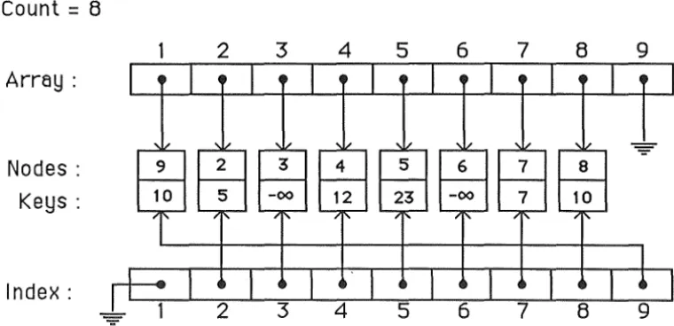
:An array ar, of pointers to records is used. Each record contains a node number and its corresponding key. A separate index array is kept so that the record of a given node can be

found immediately. A count of the number of nodes still represented in the data structure is

maintained and the structure is kept such that the pointers with indices from 1 upto this count

reference records of nodes still in the structure.

Count= 8

2 3 4 5 6 7 8

Array:

Nodes: Keys:

[image:8.600.96.476.216.400.2]

Index:

Figure 3.2 An array of pointers to 9 records, one of which (node 1)

has been deleted leaving a nil index pointer.

3.2.1 Insertion in an Array of Pointers.

9

A node and its key are copied into a record pointed to from the next available cell of the array, its index found from the incremented count of the number of items in the structure

(initially 0) i.e. the record is pointed to by ar[ count+ 1 ].

3.2.2 Deletemin in an Array of Pointers.

The array is scanned up to the current node count and the node of minimum key among those

referenced is found. The node is then removed and the corresponding pointer is made to

point to the node pointed to by the pointer contained in ar[ count ] before count is

(9)

3.2.3 Decreasekey in an Array of Pointers.

The record for the node whose key is to be decreased is found immediately from the index

array. The key is then just assigned its new value.

3.2.4 Worst Case Time Analysis of an Array of Pointers

Insertion of a record takes 0( 1 ) time since the incremented count is used as an index to the

array cell which should point to the record. Deleting the minimum record after all n records

have been inserted first involves scanning n entries, then for the next deletemin n-1 entries

must be scanned, then n-2 and so on. Thus the deletemin function for an array of pointers

priority queue actually takes n + n-1 + n-2 + ... + 2 + 1

=

(n2-n) I 2 operations, half the number of an array of keys, and so should be better when n is large enough to drown the

extra overhead. However both array methods take O(n2) time for deletemin. Decreasekey in

an array of pointers is accomplished in 0( 1 ) time because the appropriate record can be

(10)

3.3 Binary Heap

A binary heap is conceptually a tree within which every record has at most two branches and

contains a key value together possibly with some associated information such as the number of the graph node for which the key is the currently known distance. One further condition

for such a tree to be a binary heap is that the key of a record must be less than or equal to

each of the keys of the records which are contained in the left and right subtrees from that

[image:10.600.123.384.207.378.2]

record.

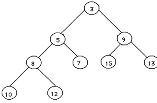
Figure 3.3 An example of a binary heap.

In the example of a binary heap in figure 3.3 each record is labeled with its key value. It can

be seen that the top record's key, 3 is less than 5 and 9 which are less than 8 and 7, 15 and

13 respectively. As a consequence of this heap order the top record of the heap contains the

key of minimum value over the entire heap.

The binary heap was represented in a Pascal array so that the parent of a record at cell i of the

array would be at cell Li I 2J of the array and so the left and right children of a record would

be at the cells with indices 2*i and 2*i + 1 respectively. A further explanation of this can be found in [HoroSahn84, 349 - 350]. The other details of the implementation proceeded

basically as described below based on this representation. The three basic operations which

need to be performed on the binary heap are described below.

3.3.1 Insertion in a Binary Heap

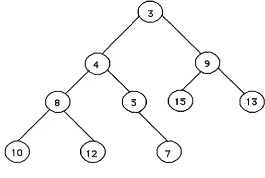
To insert a record with a specified key into a binary heap involves firstly attaching another

(11)

maintained the content of the record must be continually swapped with that of its parent until

the key of the inserted record is greater than or equal to that of its parent or it is the top

[image:11.598.115.381.140.318.2]

record. If a record with key value 4 is inserted into the binary heap of figure 3.3 then the heap in figure 3.4 results.

Figure 3.4 The heap after the record with key 4 has been inserted.

The record was attached below the record previously labelled 7 and then the contents of this

record and its parent's were swapped, putting the 7 in its final position. The key of the

record labelled 5 above was then 4 and this was less than 5, the record of its parent, so these

were then swapped and no more swapping was required because the key 3, of its parent was less than its key. It can be seen that these operations leave the structure as a binary heap

agam.

3.3.2 Deletemin in a Binary Heap

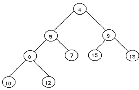
Deleting the record of minimum key value involves firstly copying the contents of the top

record and then replacing this record with the rightmost record at the bottom level. This

record is then swapped with its child of minimum key down the tree until the heap property is regained i.e. until it reaches a position where its children have keys greater than or equal to

it or it has no children. If for example a deletemin is performed on the binary heap of figure

3.4 then the binary heap of figure 3.5 would result.

In this example the top record was deleted and replaced with the record of key 4 which was

in tum replaced by the record with key 5 and the record which previously contained the key 5

(12)

[image:12.600.122.388.72.245.2]

Figure 3.5 The heap after the minimum record has been deleted.

3.3.3 Decreasekey in a Binary Heap

When the key of a record is decreased the heap order within the subtree rooted at that record

is preserved but the heap order of the rest of the heap will be disrupted if the key of the

record decreases to less than the key of its parent. So after decreasing the key of a record the

record is swapped up the tree until its key is greater than or equal to that of its parent. In the

figure 3.6 the heap of figure 3.5 has had the key of the record previously labelled 8

[image:12.600.128.405.457.628.2]

decreased to 1.

(13)

3.3.4 Worst Case Time Analysis of a Binary Heap

: Insertion requires 0( log n ) time in the worst case since an inserted record may have to be

swapped up from the bottom to the top of the tree. Deletemin requires 0( log n ) time in the

worst case since it could be necessary to swap a record from the top down to the bottom level

i.e. the full depth of the tree which for a binary tree of n records is log₂n

=

0( log n ). Decreasekey also requires 0( log n ) time in the worst case where a record at the bottom level

(14)

3.4 Alpha Heap

. The alpha heap, like a binary heap is a heap ordered tree except that an alpha heap does not

necessarily have just two branches (or less) from each record. The maximum number of

branches from each record in an alpha heap is called alpha. As with the binary heap the alpha

heap was implemented using a Pascal array. The insert, deletemin and decreasekey

[image:14.600.103.466.203.385.2]

operations are all carried out in the same way as described for a binary heap.

Figure 3.7 An Alpha Heap for a Graph with Edges/Nodes= 3.

3.4.2 Worst Case Time Analysis of an Alpha Heap

Insertion requires 0( loga.n) time in the worst case since an inserted record may have to be

swapped up from the bottom to the top of the tree. Deletemin requires 0( cxlogan ) time in

the worst case since it could be necessary to swap a record from the top down to the very

bottom level i.e. the full depth of the tree which for an alpha tree is 0( logan ). Decreasekey

requires 0( logan ) time in the worst case where a record at the bottom level has its key

decreased to a value less than the previous minimum key and hence is swapped up the full

(15)

3.5 Fibonacci Heap

-A record within this structure is contained within a doubly linked list of one or more records

all of which have the same parent i.e. they are siblings. Each record has a pointer to one of

its children from which its other children may be found by following the doubly linked list of

siblings. As well, each record with a parent has a pointer to that parent. The record in the

F-heap of minimum key is pointed to by a pointer called the min pointer through which the

entire F-heap is accessed. If the min pointer is nil then the F-heap is empty. The F-heap is

heap ordered which means that the key of every record is less than or equal to each of the keys of its descendants. For reasons which will be explained soon, each record also requires

a mark field. Thus fields for the following are required in each record :

1. The key.

2. Any associated information.

3. A pointer to its left sibling. 4. A pointer to its right sibling.

5. A pointer to one of its children.

6. A pointer to its parent.

7. Its rank i.e. a count of the number of children it has.

8. A mark field.

In order that the record for any given node can be accessed immediately an array, 'find' of

pointers to nodes indexed by their number is kept so that for example find[ 3 ] would point to

the record in the F-heap for node 3 of the graph while the node exists in the F-heap.

3.5.1 Insertion in a Fibonacci Heap

To insert a new record into the heap h, a new heap containing just the record to be inserted is

melded with h. To meld two heaps h 1 and h2, their root lists are combined into a single list

and the min pointer of the new heap is made to point to the lower of the two mins from h 1

3.5.2 Deletemin in a Fibonacci Heap

To begin with the minimum record is removed and the list of its children is concatenated with

(16)

rank they are linked. Linking involves making the root of greater key the child of the other

root. Once there remain no trees of the same rank in the list the min pointer is set to point to

[image:16.600.187.400.110.335.2]

. the new record of minimum key.

Figure 3.8 A Fibonacci Heap with minimum record of key 1.

To avoid cluttering the diagram, pointers to

parent records and nil child pointers are not shown.

3.5.3 Decreasekey in a Fibonacci Heap

To perform the decreasekey operation for some graph node x, firstly the corresponding

record in the F-heap is found from the index array and its key is decreased to the new value. Next in order that the heap order of the F-heap be preserved the record is cut i.e. detached

from its siblings and parent and is repositioned in the root list at the top of the F-heap. After

inserting this new root record the min pointer will have to be reset if the key was decreased to

a value less than that of the previous minimum key. There is a further detail necessary to

obtain the desired time bound of 0( 1 ) time for this operation. During a deletemin, when a

root record is made the child of another record in a linking step, as soon as two of its

children are cut by a decreasekey operation it must also be cut. The mark field is used to keep

track of the number of children a record has lost due to cuts. During a linking step the child

record is unmarked.When a record is cut, if its parent is unmarked then it is marked

otherwise if its parent is marked then it too is cut. In this way it is possible for a decreasekey

(17)

3.5.5 Worst Case Time Analysis of a Fibonacci Heap

-Insertion requires 0( 1 ) time. Deletemin requires 0( log n ) amortized time in the worst case. Decreasekey requires 0( 1 ) amortized time in the worst case. The analyses for these are

(18)

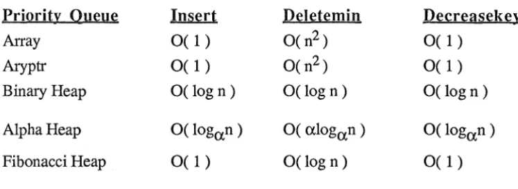
3.6 Summary of Worst Case Time Analyses

Figure 3.9 summarises the time bounds found for each of the priority queues discussed

above. Clearly the Fibonacci heap exhibits the best time bounds, it being the only priority

queue with a bound equal to the best of the others for each of the three operations.

PriQritx Q:ueue Insert Deletemin De~reasekex

Array 0( 1) O(n2 ) 0( 1)

Aryptr 0( 1) O(n2 ) 0(1)

Binary Heap O(log n) O(log n) O(logn)

Alpha Heap 0( logcx,n) 0( cx.log₀

p )

0( logan) [image:18.600.102.476.180.317.2]

Fibonacci Heap 0( 1) O(log n) 0( 1)

(19)

Given a graph with n nodes and m edges each with some associated non-negative cost this

algorithm can find the distance from a specified source node to all the other nodes in the

graph. The distance from one node to another is the minimum cost of traversing any path

between them. Dijkstra's algorithm works in conjunction with a priority queue for storing the

currently known distance of each node from the source. These distances are updated by way

of the decreasekey operation and once the distance to a node is known it can be deleted by

way of the deletemin operation.

As the latter sentence suggests Dijkstra's algorithm finds each node in order of

non-decreasing distance from the source. Initially the source is inserted in the priority queue with a key of 0, since it is known that there is a cost of O in travelling from the source to

itself, and all other nodes are inserted with a cost of oo. The algorithm then loops n times, in each finding the next furthest node from the source and updating the keys of other nodes. If

we denote the cost of the edge (p, q) from node p to node q by cost(p, q), the current key in

the priority queue of a node q by distance( q ) and the decreasekey operation by decreasekey(

q, newkey) meaning that node q has its key decreased to the value newkey then we may write Dijkstra's algorithm in pseudocode as follows:

Insert source node with key = 0.

Insert all other nodes with key= oo.

While the priority queue is not empty :

Deletemin, giving the node, p and distance, d

Assertion: The distance to node pis d.

For each node, q adjacent top:

If d + cost( p, q) < distance( q) then decreasekey( q, d + cost( p, q ))

Further more detailed explanations of how and why Dijkstra's shortest path algorithm works

(20)

4.1 Worst Case Time

. From the above pseudocode it can be seen that for a graph of n nodes and m edges there will

be n insert operations, n deletemin operations and in the worst case there will be a total of m

decreasekey operations. Thus the worst case time for Dijkstra's algorithm using any given

priority queue is:

WCT( Priority Queue )

=

0( n

*

insert + n

*

deletemin + m

*

decreasekey ) [1]

where insert stands for the time to perform the insert operation, deletemin stands for the time

to perform the deletemin operation and decreasekey stands for the time to perform the decreasekey operation, all in the worst case. Generally by worst case we mean that situation

in which the operation will require the maximum possible time.

The behaviour of Dijkstra's algorithm on three particular types of graph were investigated. The first of these was sparse graphs where the number of edges is small compared to the

number of nodes i.e. m

=

0( n ). These are of interest simply because large graphs often have few edges per node e.g. communications networks or the roads in a country where each

node only has edges to those nodes near it; Dense graphs where m = 0( n2 ) are of interest

simply because they represent the other extreme. No runs were made of Dijkstra's algorithm

on dense graphs since the result, that an array-type priority queue performs best, is well

known. In between these two extremes there are, as they shall be refered to in this report,

middle graphs. A middle graph has an edge to node ratio of the order of the log of the

number of nodes i.e. m

=

0( n

*

log n ). These are of interest because it is on such a graph that the Fibonacci Heap has an asymptotically superior time bound and hence should be

faster than the other priority queues, provided that the number of nodes is sufficiently large. By substituting the time bounds, summarised in figure 3.9, into equation [l], the worst case

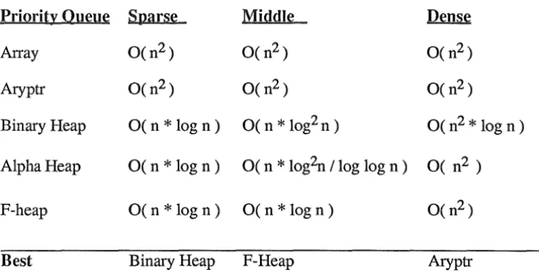
time bounds for Dijkstra's algorithm may be found. These are summarised in figure 4.1,

below. It can be easily derived that for an alpha heap the best choice of alpha when used in

Dijkstra's algorithm is

a.=

m/n. The last row of the table in figure 4.1 gives the fastest

priority queue, assuming sufficiently large n, for each of the three categories of graph,

namely sparse where m

=

0( n ), middle where m

=

0( n

*

log n ) and dense where m

=

0( n2 ). It can be seen from this that the F-heap is asymptotically superior to the other priority

queues for graphs with O(n

*

log n) edges. For the sparse graphs, although the three heap methods take the same order of time, the binary heap has the least overhead and so should be

(21)

Priority Queue Sparse Middle Dense

Array O(n2 ) O(n2 ) O(n2 )

Aryptr O(n2 ) O(n2 ) O(n2 )

Binary Heap 0( n

*

log n) 0( n

*

log2n) O(n2

*

log n)

Alpha Heap 0( n

*

log n) 0( n

*

log2n I log log n ) 0( n2 )

F-heap 0( n

*

log n) 0( n

*

log n) O(n2 ) [image:21.600.118.502.84.277.2]

Best Binary Heap F-Heap Aryptr

Figure 4.1 The time bounds of the priority queues for graphs of different edge densities.

(22)

,~-~-~~-.-,---5.1 Graph Representation

To represent the graph in the computer's memory an adjacency list is used. This is an array

of linked lists indexed by node number. For each node adjacent to a node, x the linked list

pointed to by entry x of the array contains a record for that node. In this way it is possible to

visit every node adjacent from some node by just traversing the corresponding list and

furthermore this can be done in the least order of time possible, each access to a node being

0(1). The construction of this list is also very efficient, taking just 0( m) time. If instead a cost array, c is used where c[x,y] is the cost of the edge from node x to node y then O(n2 )

time would be needed to initialise it and O(n) time would be needed to visit every node

adjacent from some node, x by scanning row x of the array.

2

3

4

5

6

[image:22.600.162.351.298.511.2]

4

Figure 5.1 A graph and its adjacency list representation.

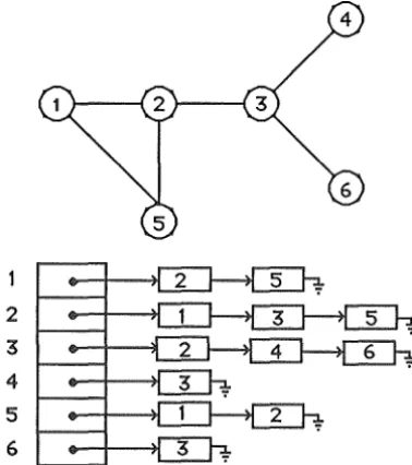
5.2 Worst Case Graph

In order to ensure the maximum possible number of decreasekey operations and worst case

time for a decreasekey operation on each data structure it was necessary to find a graph cost

function such that the tentative distance to each node as found by Dijkstra's algorithm would

(23)

6

5

[image:23.600.160.392.87.232.2]

10

Figure 5.2 A worst case graph for n

=

5

In this example it is assumed that Dijkstra's algorithm scans all the edges from a node in

order of decreasing number of the adjacent node that is right to left in figure 5.2. Initially

nodes 2 to 5 are inserted into the priority queue with cost infinity and node 1 is inserted with cost 0. Next assuming that node 1 is the source node the following is a trace of what happens

when Dijkstra's algorithm is applied:

Current Nsu!g Adjacent NQdg Old Ke)'. Ne:Il'. Kgl'.

1 0 <--deletemin

1 5 00 10

1 4 00 9

1 3 00 8

1 2 00 1 <--deletemin

2 5 10 7

2 4 9 6

3 5 7 5

Figure 5.3 An example of running Dijkstra's algorithm for a

[image:23.600.81.484.402.620.2]

(24)

Notice that each time a key value is updated by a decreasekey operation it changes to a value

less than the current minimum, so that within the heap structures the associated node must be

-repositioned at the top of the heap which results in the worst possible time performance.

Generally a graph of n nodes with the cost function shown in figure 5.4 will produce the

worst possible behaviour of Dijkstra's algorithm using any of the priority queues provided

that the source is node 1.

} q

p

+

1

cost(

p, q)

} p

<

q

[image:24.598.112.472.193.347.2]

any

k

2 0

} p

2

q

Figure 5.4 The worst case cost function.

s

. · · ·

-ll.-1 S=Ii

)

S-1

s-n

S-n+1

[image:24.598.98.434.438.650.2]

(25)

As is shown in figure 5.5 a worst case graph with n nodes and n

*

(n - 1) I 2 edges is formed

by the algorithm described in the following pseudocode :

nextcost ~ 2

For each node i from 1 to n-1 :

cost( i, i+l) ~ 1

For each node i from n-2 downto 1 :

nextcost ~ nextcost + 1

For each node j from i+2 ton :

cost( i, j ) ~ nextcost

nextcost ~ nextcost + 1

From the edges given to the graph by this algorithm, m needed to be chosen. The n-1 '1'

edges between adjacent nodes were left to ensure that the nodes were deleted from the

priority queue in the correct order. From the other nodes, m - n + 1 edges had to be chosen.

Since this choice was unimportant, in that any choice would yield a graph which would

result in m worst case decreasekey operations, the choice was made deterministically. This was done by adding the 'l' edges and then spreading the remaining edges evenly over the

remaining nodes. To accomplish this spreading of edges, the average p, of edges left per

node was found and was used to find k == n - p - 2, the number of the node after which less

than p more edges can be added because of a lack of destination nodes. All corresponding

edges were then added to the nodes from k+ 1 to n-2 and the average p, of edges left over the

remaining k nodes, was calculated. For each of the nodes i from k down to 1, the p shortest

edges of the worst case graph, with the node i as source, were added until the graph

contained m edges. In this way a worst case graph of n nodes and m edges was created in

(26)

The programs needed for this project were written in Pascal with each priority queue a

separately compiled unit and were executed on the Prime750 of the Computer Centre at the

University of Canterbury. The measurements made were of the time for Dijkstra's algorithm to run and of the number of comparisons between keys and accesses of keys. The latter is

important because although in the case of Dijkstra's algorithm the keys are simply numbers,

the priority queues could be used for algorithms where the keys are objects for which comparisons and/or accesses require a great deal more time, for example they might be large

records. Due to limitations of memory it was not possible to generate graphs of more than 2500 nodes. A graph of 2500 nodes is the largest and hence most interesting for which

(27)

All the results given in this report are averages over 10 runs. Some of the results are tabulated in the appendix. If necessary, further details may be obtained from the author.

7.1 Results Shown In Graph 1

Graph 1 shows the time taken by the five priority queues when Dijkstra's algorithm was run

on worst case graphs of 100 nodes with edges per node varying from 2 to 10. The array

priority queues clearly become faster than the others. This is due to the low overhead in these methods compared with that of the other three. Of the array methods aryptr is faster, even

though it has a little more overhead, since the n deletemins only require half as many

operations (see section 3.2). Although fastest here, the results for a worst case graph of 500

/' \

nodes shown on page A+ 12J>f the appendix demonstrate that the arrays, as expected,

eventually became much slower than the other methods. Consequently the array priority

(28)

<,< v'IAC ul'AP~ PAPE HS Cl FW, Cltu lCfl N ,l B 101Y IOt 1 ' , & inc.i

(\::=. \UO ~

. I

1

r

f

l

l '

I

.

I

f

I

i

LI

l

-2

I

-2·S-t

-

t

l

I

I I I

I

I I

f

I

+

1

J

t

l

I

. . ·,: .

·.-.·.--· -.·.--·

.. ·.-,-.· -· .. ··---· ..

. . 1· _.; ·_-_:

(29)

7.2 Results Shown In Graph 2

-Graph 2 shows the time taken by Dijkstra's algorithm using the priority queues on a graph of

2500 nodes with edges per node varying from 2 to 20. From edges per node= 4 to 13 the

F-heap is the fastest of the priority queues. As m In= Iog₂(2500) z 11, this range agrees

with the best value of m for an F-heap predicted from the theory. For min= 14 the alpha heap becomes the fastest of the priority queues because of a sudden drop in the time taken

from min = 13 to min = 14. This drop is explained by a decrease in the depth of the alpha

heap; at min= 13, a= 13 so the depth is

r

loga(n (a - 1) + 1)

l

= 5 while at min= 14, a=

14 so the depth is

r

loga(n (a - 1) + 1)

l

= 4. With a lower depth the alpha heap requires less time to swap records from the top to the bottom and vice versa in deletemin and

decreasekey operations, respectively. Nevertheless swapping nodes toward the bottom of the

heap in a deletemin operation requires requires scanning

a

records for the one of minimum

key at each swap. Hence apart from drops in the time required, due to the depth decreasing,

the time taken generally increases as a increases. There will be similar drops in the time

taken when the heap depth decreases from 4 to 3 and from 3 to 2, these will occur from

branching factors of a= 50 to a= 51 and a= 2498 to a= 2499. Although there are drops

in the heap depth for regions shown in the graph other than the one cited above, these earlier

drops had less of an effect on the time taken since the decrease was less in proportion to the

initial depth.

(30)

C,O !MAC. G11AI H PAPE m, . Cl-ti It ! L,I llflC,ll ~ l 8101'( •Gt 1s," & 1111rh

:_:·\,.•, ~ .

i:'

\'

-

~--:

::·:.~--· ...

;--

(31)

,.3 Results Shown In Graph 3 and 4

Graph 3 shows the number of key comparisons made by each of the three heap priority

queues used in Dijkstra's algorithm on a worst case graph of 2500 nodes. Clearly the F-heap

makes far less comparisons between keys than the other priority queues. From the results

listed on page A-5 of the appendix it can be found that the Fibonacci heap varies between

making 1.2 to 2.6 less key comparisons than its nearest rival the alpha heap. The sudden

drop in the alpha heap graph from

ex.=

13 to 14 can be explained as in 7.1 by a decrease in

the depth of the heap.

Graph 4 shows the number of key accesses made by each of the heap priority queues for

worst case graphs of 2500. These show that there is little difference between the three

methods in the number of accesses. Although the binary heap makes the fewest accesses this

is not a significant advantage as it only makes a few thousand less than the F-heap which

makes a few hundred thousand less key comparisons than the binary heap. Key comparisons

are likely to take much greater time than accesses in any case. The graphs show that the

binary heap makes the fewest accesses followed by the F-heap and the alpha heap makes the

(32)

t,ORl\r.'\CK CiflAPh PAPE 1; CHtU;:, fC.lUHC IN.,-.

t

I

BlOY 10tl,,i',&111c~

()

.,,.r " ~ 2..'SOO.

I

I :J,O

··:--:-~:--:-·.-_

. ·. -'-.. --

...

·

.. ·•· . ·: ..

-.-.:".·;-···.

-·".',.. .·

I,.

1-· • . • ·;..·

• -.•r',,•

(33)

dRMAC~ C, lAPH FAP R5 : C'Hlll5TC HJHU• N.l.

I

t

!

0

l

f

t

l

t

' 1

t

j

i

!

I

! I I

I I

t

l

!

r;l'>lY 101i,.~llt 1 net

'f

I

t

!::: ,, :

r --~ .,· .

~--~; .. ,( .... :·:;:.

l

r

: '. ..

l

. : .:

(34)

-7,4 Results Shown In Graphs 5 to 7

Graphs 5 through 7 show the performance of the three heap priority queues for varying

numbers of nodes with the number of edges kept constant at n

*

log n. Graph 5 shows that

the F-heap only just gives the best time for a worst case graph of 2500 nodes. Graph 6 shows that the F-heap makes significantly less key comparisons than the other methods

while graph 7 shows that there is little difference in the number of key accesses made by each

priority queue, relative to the other considerations as explained in section 7.2 above.

These three graphs demonstrate that if Dijkstra's algorithm is applied to a worst case graph of

n nodes and n

*

log n edges, the alpha heap used as a priority queue gives the best time

(35)

<iOl~MACKCiRAPHFAP RS CHU,fC'HJl~Cf-iNZ. B OlY 101.,,,,P~ t nc~

,

Srof~

S

.

1

f

I

H

I

H

I

!

1

I

_I

' l

t·>

I

! I

I

_l

~

+

i I

~.-:-~ ...

-t • - -...

.

. . . ·-·

(36)

. i ; I

!

.

t

. _

_

t

I

f

l

.

r

I

_

~

I +

~

I .

f

t

~

..

t

·

:

· .

t

I

f

I

t

I ' . I

I

I I '

l . I : l . I ~ ' ' ' ' I I I I

l

i . ;

raf7o(V

·

f

c>

J;;,f

.

·

frYl{V

f?o/

.

r

~

...

! I.

I I I + I . T .

t

r

1 L

~

rt

I

t j+

~r1·

I

if

:

l'

'

t

.

t

I

r

1 : 1 3

_H.

!

t

I

L

.

f, :

N

.

rj

'

L

!

b

1 [ '. ·

l

j

l

I

I I I ' I : , 1

:i

!

I

)

it

:

!1

t

)

:f

1

!

1

+ .

b

,

k,

t

:

~

I . · \ I

~

. I T

.

1,

I

. I 1 1

j

+ I

t

'

t

J 1. I

'

; I:

i'.

I

t

'

rt;

1·;:

,

'

1

i

r'1·

1

1 f : : -'. ! I

JI

t

1 +

~

1

.

}

' j J

f

. •

.

:

I

~

+ . . c I I

I

t

I [

~

()I . ! · 1

it

f · · -r 1 1 =

l.

1 ~ . : : +

r

ii

l

r

I

.

~

'

tl

I . r . :

t-1

1

,

u

,

t

I

• I , I I

,

t

C i ~ I _ '.. .

I

I I . ,. I ~ t + I

t

I : . • ] .J., , c . •. I i. •

i

i ~ r ><

l

r ! ·

I

f

•.

:

·

=

j

~

t

t ,

-~

~

.

1 .. '

/f

f.

r

· 1 _ , . t I

I

~ : I f" I . I • t' I 1 :~

,

i

!

t

ti + ,, = :

t

~

'!

'

'I

jl

I i

1

~·,.i,

1

tf

.

yr

11

l

11.111·

1

-i!

:1t

,

f

:1r;i·

· t r

!

'

~

r

J .

· ·1

~

· 1

I

·

c

·

f

t

. • ' .. :- ' j-

•

.

t

.

-~

.

t

f

. .._I ·/

I ~ : · : . [ • · ~ ' '. : ' I I : t t

I

.

"

.

f

I

:mvr~

1

~

(

t

'

_t[

,

1

f

.

f

J

!

[

1! ,

t{I

I

1i

l

l1L

ll

llJ

ll

il

l

Jlt

i

fj

IJ

•

1

·

.I Irr

:-·. - ··-· _ · j i :_ ;_ : ·· . :::: ----=-~ .· :~ ,

"''"'

T [

- -- ~ -. · . ··"'. -... . . :.;: ::. : . : . :_: - ·..·.. \,.-· .

I ,

,.

.

..

r

l

ti r .

t

1 . i + •. I .

I

~

·

··

·

t

~

• t-

I

l I r

~ . ' j c L i 1. 1 ~ I . . . • J ~ . ~

s

f

n

[

I '

'

7

t

)

I" . . I . I t

WM

·

~~

'

"'!Cl

I

I " I

I l

I

'

-I

J<

1

4J

i

.

I 1

00!

1

l

;~

t

J_~~,,'

1

,J

,

u

!AMd»

/

!

1

J

l

,'

~

1

:

.

l~J

;

!

)

~~t

(37)

UORVACK FIAPI .'APE RS Cl1_{Hl5 CHu lC l NZ}

t

i

8101Y 10t 1s h & I 111c11

N

o

l

_I

r

1

... -~--·.

:.:_~-~----~·-:.

,.

i · . .

f:_cc:. · ..

i I ..

t .•• ~

(38)

7 .5 Summary of Results

-Figure 7 .1 shows the best priority queue for varying numbers of nodes and varying densities

of edges for Dijkstra's Shortest Path algorithm applied to a worst case graph. The last

column indicates the well known result that arrays are fastest when used for dense graphs.

Node~ Snarse Granh Middlf Gra12h Den~f Granb

500

Binary Heap Alpha Heap Aryptr

1000

1500

2000

Binary Heap Alpha Heap Aryptr [image:38.600.116.498.161.274.2]

2500

Binary Heap Fibonacci Heap Aryptr

Figure 7.1 The fastest priority queues for a worst case graph.

These results apply to integer keys. If however the keys are very large and hence take much

longer than do integers to be compared then the Fibonacci heap is likely to be significantly

faster than the other heaps in areas where it is not shown to be in figure 7 .1 since the Fibonacci heap was found to make greatly fewer key comparisons for both sparse and

(39)

8.

Conclusion

The project was successful in showing Fibonacci heaps to be faster than other commonly

used priority queues when used by Dijkstra's Single Source Shortest Path algorithm on

sufficiently large worst case graphs. It was also found that the F-heap makes significantly

less key comparisons than the other methods, which consequently would make it even faster,

(40)

References

[FredTarj84] M. L. Fredman, R. E. Tarjan; "Fibonacci Heaps and Their Uses In Improved Network Optimization Algorithms", IEEE

Computer Society 25th Conference on Foundations of Computer

Science, Oct 1984, 338 - 346.

[HoroSahn84] E. Horowitz, S. Sahni; "Fundamentals of Data Structures

in Pascal", Computer Science Press, 1984, 349 - 350.

[AHU74]

[AHU83]

A. V. Aho, J.E. Hopcroft, J. D. Ullman;

"The Design and Analysis of Computer Algorithms",

Addison-Wesley, Reading, Massachusetts, 1974, 207 - 209.

A. V. Aho, J. E. Hopcroft, J. D. Ullman;

"Data Structures and.Algorithms", Addison-Wesley, Reading,

(41)

(42)

Time in CPU Seconds for Nodes= 2500, Edges per Node= 2 .. 20. Edges/Node

2.

4.

6.

8.

10. 12. 14. 16. 18. 20. Binary Heap 3.063 4.846 6.778 9.464 9.028 10.359 12.111 13.842 15.697 17.212 Alpha Heap 4.053 5.071 6.933 9.730 11.071 14.412 18.727 21.048 24.042 25.607 Fibonacci Heap 3.352 4.664 6.267 8.321 9.886 11.555 11.730 13.280 14.781 16.142

Time in CPU Seconds for Nodes= 2000, Edges per Node= 2 .. 20.

Edges/Node

2.

4.

6.

8.

(43)

Time in CPU Seconds for Nodes= 1000, Edges per Node= 2 .. 20. Edges/Node

2.

4.

6.

8.

(44)

Number of Key Comnparisons for Nodes = 2500, Edges per Node= 2 .. 20. Edges/Node

2.

4.

6.

8.

10. 12. 14. 16. 18. 20. Binary Heap 76346. 100704. 128692. 173479. 83169. 97677. 115130. 132043. 150618. 165362. Alpha Heap 76346. 92834. 125692. 174698. 191589. 247177. 318590. 354806. 403164. 421731. Fibonacci Heap 29264. 42118. 57539. 148873. 173483. 203126. 205578. 232122. 257485. 279207.

Number of Key Comnparisons for Nodes = 2000, Edges per Node = 2 .. 20.

Edges/Node

2.

4.

6.

8.

Edges/Node Binary Heap Alpha Heap Fibonacci Heap

2. 42889. 42889. 17022.

4. 57344. 54460. 24734.

6. 74328. 68051. 33992.

8. 105147. 84527. 43583.

10. 126929. 100976. 53613.

12. 139324. 103750. 63009.

14. 171388. 120323. 73713.

16. 174651. 134631. 84066.

18. 220162. 147742. 94431.

20. 255624. 159917. 103710.

. '·.~. '. • ,

(45)

Edges/Node Binary Heap Aloha Heap Fibonacci Heap

2. 26556. 26556. 11164.

4. 35535. 33896. 16305.

6. 47284. 44033. 22482.

8. 57444. 53765. 28874.

10. 78554. 58377. 35559.

12. 90631. 68357. 41828.

14. 112690. 77503. 48965.

16. 126132. 85788. 55867.

18. 134081. 92883. 62771.

20. 144448. 98878. 68971.

(46)

Number of Key Accesses for Nodes == 2500, Edges per Node == 2 .. 20. Edi:es/Node 2. 4. 6.

8.

Number of Key Accesses for Nodes == 2000, Edges per Node == 2 .. 20.

Edges/Node

2.

4.

6.

8.

Number of Key Accesses for Nodes== 1500, Edges per Node== 2 .. 20.

(47)

Number of Key Accesses for Nodes = 1000, Edges per Node= 2 .. 20.

2.

4.

6.

8.

Number of Key Accesses for Nodes = 500, Edges per Node= 2 .. 20.

(48)

-Ed1,rns/Node Array Aryptr Binary Heap Alpha Heap Fibonacci Hean

2. 0.126 0.099 0.090 0.130 0.137 3. 0.133 0.104 0.124 0.152 0.166 4. 0.143 0.112 0.153 0.186 0.200

5.

0.151 0.123 0.195 0.198 0.238 6. 0.159 0.131 0.228 0.225 0.270 7. 0.168 0.141 0.253 0.252 0.314 8. 0.176 0.147 0.297 0.280 0.350 9. 0.184 0.157 0.341 0.302 0.394 10. 0.193 0.165 0.368 0.322 0.431

Number of Key Comparisons for Nodes = 100, Edges per Node = 2 .. 10.

Edges/Node Array Aryptr Binary Heap Alpha Heap Fibonacci Heap

2. 9900. 4950. 1698. 1698. 932.

3. 9900. 4950. 2118. 1995. 1191. 4. 9900. 4950. 2523. 2487. 1448.

5.

9900. 4950. 3069. 2626. 1797. 6. 9900. 4950. 3489. 2914. 2067. 7. 9900. 4950. 3764. 3231. 2392. 8. 9900. 4950. 4375. 3597. 2709. 9. 9900. 4950. 5082. 3882. 3089. 10. 9900. 4950. 5401. 4101. 3375.

Number of Key Accesses for Nodes = 100, Edges per Node = 2 .. 10.

Edges/Node Array Aryptr Binary Heap Alpha Heap Fibonacci Heap

2. 899. 795. 601. 1096. 811.

3. 1099. 1042. 801. 1175. 1011.

4. 1299. 1289. 1001. 1374. 1226.

(49)

Time in CPU Seconds for Edges = n

*

log n.

Nodes Edges Binary Heap Alpha Heap Fibonacci Heap

500. 4483. 2.072 1.631 1.971

1000. 9966. 4.795 4.013 4.341