Application of Particle Tracking in Large Scale Timber Connection Testing

APPLICATION OF PARTICLE TRACKING IN LARGE SCALE TIMBER

CONNECTION TESTING

Lisa-Mareike Ottenhaus

_{, Minghao Li}

_{, Roger Nokes}

ABSTRACT: Particle Tracking Velocimetry (PTV) is a quantitative field measuring technique originally designed to track individual particles in fluid flows. In this study, PTV was applied for the first time in the context of large scale timber connection testing. The suitability of PTV in structural applications was assessed by tracking the attachment points of string potentiometers and comparing the PTV displacements to those obtained by the potentiometers. Furthermore, it was found that PTV was able to capture crack growth and compute the resulting displacement field in the connection area.

KEYWORDS: Particle Tracking Velocimetry, Digital Image Correlation, Mark Tracking Method, Timber Connections

1

INTRODUCTION

The idea of contact free strain and displacement field measurements by means of Digital Image Correlation (DIC) dates back to the end of the last century [1] when images were captured on film and then digitalized. DIC was successfully applied in structural timber engineering in the 1990s [2, 3]. In simple terms DIC works by comparing two digital images of the test specimen’s surface before and after deformation. The light intensity pattern of a pixel subset of the undeformed image is stored and recognized in the deformed state. By cross-correlating several subset pairs a strain or deformation field can be calculated [4]. Nowadays, DIC is widely applied in research and practice. For instance, it has been successfully combined with FEM [5-7] and has been used in practice to monitor building deformations [8]. DIC has the advantage that it doesn’t require special lighting and timber surfaces don’t require any preparation. However, the quality of the data obtained with DIC relies on the subset size and correlation function and can suffer from noise during image acquisition and processing [9].

A variation of the DIC technique is the Mark Tracking Method (MTM) where marks or dots are applied to the specimen surface and tracked over time [10, 11]. Tracking distinct marks can be an effective way to eliminate noise in practice applications and facilitate the

1-3 _{University of Canterbury, Department of Civil and Natural} Resources Engineering, Private Bag 4800, Christchurch 8140, New Zealand, 1_{[email protected]} 2_{[email protected]}

3_{[email protected]}

tracking of discontinuous processes such as crack growth and fracture.

Particle Image Velocimetry (PIV) and Particle Tracking Velocimetry (PTV) are both quantitative techniques originating in fluid mechanics designed to measure velocity fields within fluid flows. Both techniques are based on the principle of capturing video images of a particle seeded fluid flow, and from that video record extracting quantitative information about the flow field [12, 13].

PIV is based on the cross-correlation of the intensity fields in two consecutive frames, with fluid velocities obtained from peaks in the cross-correlation field. PIV is very similar to DIC, except that in DIC the medium is solid and deformations are mapped. Recently, PIV has successfully been implemented in structural timber engineering to visualize stresses and strain fields in a deforming Cross Laminated Timber (CLT) slab [14]. PTV on the other hand is more similar to MTM as it identifies individual particles within each frame which are then tracked from frame to frame in order to establish particle-centred velocity estimates. For structural applications this has the advantage that a movement path is created for each individual particle. In the context of timber connection testing this allows for a displacement field to be measured while simultaneously tracking the movement of fasteners or instrumentation attachment points.

research, thereby replacing conventional LVDTs (Linear Variable Differential Transformers) and potentiometers while also providing more data quantity with the potential of improving the data quality.

2

EXPERIMENTAL SETUP

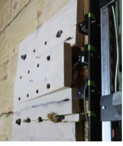
A total of 12 large scale connection tests were conducted on CLT panels at the Structural Engineering Lab of the University of Canterbury. The connections consisted of an internal steel plate as well as 12 smooth steel dowels and 4 dowels with threaded ends and nuts and washers in the corners. Two different connection layouts and two different CLT layups were subjected to monotonic and cyclic loading in axial direction via two hydraulic jacks (Figure 1). The panel rested on roller supports and the internal steel plate was connected to a reaction frame. The main research objectives were:

- Evaluation of ductility and overstrength of large scale dowelled connections in CLT panels under monotonic and cyclic axial loading. - Comparison of findings to previous research on

small scale connections [17-19]

- Monitoring of overall connection behaviour by means of PTV and quality assessment of PTV measurements in a structural engineering context.

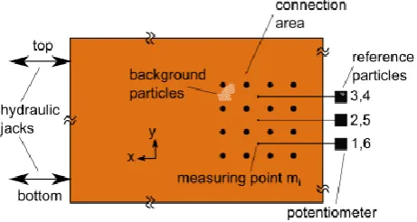
The detailed test setup and experimental findings as well as discussion of the first two research objectives can be found in a different publication [20]. The present paper focusses on the third research objective. In order to provide a more in-depth evaluation of PTV only findings from connection 04 are discussed in the following. This connection was subjected to cyclic loading according to the ISO loading protocol [21, 22] in the x-direction as indicated in Figure 2.

Figure 1: Experimental setup

2.1 INSTRUMENTATION

It was decided to evaluate the overall connection behaviour by means of PTV as well as traditional rotary string potentiometer measurements. For this purpose a

fine mesh of matt white background particles was applied on each panel side as shown in Figure 2. Additionally, three string potentiometers were mounted at the centreline of two dowel rows at each panel side. The potentiometer resolution was 0.15mm/count with a +/-0.25% accuracy. The draw-wires were attached to matt black coated screws at the centre of the connection. These measuring points also served as PTV particles in order to directly compare PTV measurements, mi, to

potentiometer measurements, pi. Several reference

particles were applied to each potentiometer mount in order to monitor and later subtract ambient vibrations.

Figure 2: Instrumentation

3

METHODOLOGY

PTV in structural testing consists of the following three main steps:

Preparation

- Particle application - Camera setup and lighting Experiment

- Image capture

Post processing and analysis:

- Image processing and particle identification - Particle tracking

- Displacement (field) generation

Some practical guidance is given in each step described in the following sections.

3.1 PARTICLE APPLICATION

Particles should have sharp edges and sufficient contrast from the substrate in order to facilitate particle identification. In general, matt paints should be used to avoid reflections. In this study, a regular pattern of matt white paint dots (1.5 mm diameter, 2.5 mm spacing) was applied onto the timber surface. These background particles served to capture the overall timber surface behaviour, local crushing around the dowels, and crack growth.

The dowel heads and screws where the draw-wires were attached were also coated in matt black paint. These black particles served to track individual fastener movements and to compare PTV measurements to potentiometer readings.

ambient background vibrations. A reference scale was drawn onto the specimen which served to translate image pixels into millimetres.

It should be noted that random particle patterns are generally easier to track and recognize than regular patterns. Furthermore, the particle pattern can be varied to reduce the total number of particles. Other possible patterns could consist of fine particle patterns close to fasteners and a coarse and sparse mesh in the surrounding areas to analyse the connection behaviour as a whole. Likewise it is possible to apply a fine background mesh and analyse small “interesting” areas in detail while applying a coarse mesh of different size or coloured particles to obtain global connection behaviour without having to process vast amounts of data.

3.2 IMAGE CAPTURE

3.2.1 Camera equipment and lighting

The quality of the data strongly depends on the quality of the captured images. Image distortion, shadows and varying intensity in lighting should be avoided in order to minimize the amount of required post processing. For this research two Canon EOS 750D DSLR cameras with an EFS 18-135 lens were mounted on sturdy tripods at each side of the test panels. The cameras were level with the centroid of the connection area at approximately 1.5 m distance from the specimen surface. Fluorescent light racks were mounted beneath the cameras to eliminate shadows and provide consistent lighting conditions. It should be noted that it is important to adjust the camera shutter speed such that it captures at least one complete cycle of the light frequency to avoid drastic changes in image brightness. Furthermore, aperture, ISO speed and camera focus should be set manually in order to avoid changes between images. 3.2.2 Camera trigger

The data and image acquisition were synchronized and triggered every 2 seconds. A time trigger was chosen instead of a load or displacement dependent data trigger to obtain more consistent data as the hydraulic jacks could not be moved with a constant displacement rate. 3.2.3 Image resolution and PTV accuracy

The resolution of the images was 6000x4000 pixels. The PTV resolution ranged from 0.19 to 0.26 mm/px depending on the size of the captured connection area. This resolution was slightly lower than the resolution of the string potentiometers which was 0.15 mm/count. This loss in accuracy was deemed acceptable as the main goal of the research was to capture overall connection behaviour. However, the resolution can obviously be increased by using two or more cameras per connection side and zooming in on different areas.

3.3 IMAGE PROCESSING

3.3.1 Particle Identification

A particle is identified through differences in light intensity. Additionally, shape, size and colour can be used to distinguish between those pixels lying within and

outside of a particle. Either a grey scale or RGB spectrum intensity analysis can be conducted to compute the light intensity of an area containing n pixels. The particle’s location is then defined by the centre of gravity coordinates (xg, yg) of the pixels that lie above a certain

intensity threshold as shown in Equation 1:

n i I I H I I H y y I I H I I H x x

i i s

i i i s

g

i i s

i i i s

g  1 ) ( ) ( ) ( ) (              









where (xi, yi) are a pixel’s coordinates, Iiis the pixel’s

intensity level, Is is the intensity threshold and H is the

Heaviside function as defined in Equation 2. This analysis is repeated for each image. Figure 3(a) displays the identification of the background particles close to measuring point m2 and Figure 3(b) and (c) display the

identification of the measuring point itself.

(a)

(b) (c)

Figure 3: Particle identification

3.4 PARTICLE TRACKING

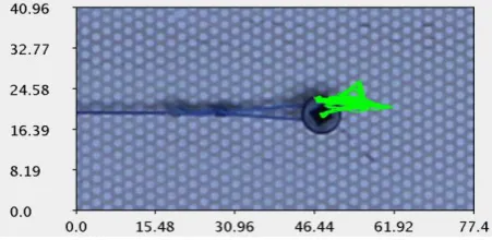
3.4.1 Particle matching

A particle path is created by matching particles between images and storing their location for each image. In the given case, particles were matched based on their horizontal and vertical distance between images. Spurious particles were removed based on the total length of their path. Figure 4 shows the movement path of measuring point m2 throughout the entire experiment.

3.5 Removal of background vibrations

As shown in Figure 2, reference particles were applied to each potentiometer mount in order to capture movement of the cameras and ambient background vibrations of the entire experimental setup. A path field was computed for each set of reference particles and their average was subtracted from the respective measuring point path in order to obtain the relative movement between the measuring point mi and the potentiometer mount. It is

important to ensure that both reference particles and the particles of interest are captured within the same image as different cameras could be moving differently.

3.6 DISPLACEMENTS

3.6.1 X- and y-displacements of measuring points Each particle’s location (xk, yk) is stored for each time

step t. In the given case an image was taken every 2 seconds and therefore t has a physical meaning. For displacement or force triggered image acquisition a pseudo time step can be used to refer to an image’s position in a sequence of images.

In order to compare PTV results with potentiometer readings, 6 measuring points m1...6 were tracked over n

time steps t. The measuring point’s x- and y-location with respect to its origin, mix and miy, were then

calculated by Equation 3. As a potentiometer is only capable of measuring its string elongations, the total distance from the origin mi was calculated by Equation 4.

n t i y t y t m x t x t m i i iy i i ix 

6; 0

0 ) 0 ( ) ( ) ( ) 0 ( ) ( ) (          (3) n t i t m t m for t m t m t m t m t m ix ix iy ix iy ix i 

6; 0

0 0 ) ( 0 ) ( ) ( ) ( ) ( ) ( ) ( 2 2 2 2             (4)

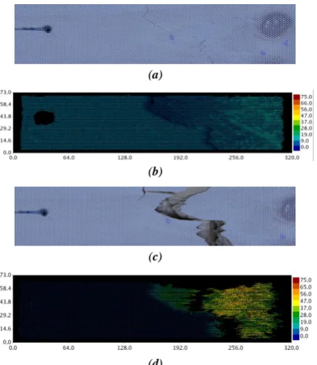
3.6.2 Displacement fields

Streams 2.06 is capable of calculating displacement fields from individual particle paths by triangular interpolation, similar to the Finite Element Method. Displacement fields are useful to visualize dowel embedment or crack growth. In connection 04, a crack developed next to m2. Figure 5(a) shows the start of the

crack growth and Figure 5(b) displays the respective cumulative displacements. Figure 5(c) and (d) on the other hand display the fully developed crack and respective displacement field towards the end of the experiment.

(a)

(b)

(c)

(d)

Figure 5: Crack growth and cumulative displacement

fields close to m2 in connection 04.

4

RESULTS AND DISCUSSION

The accuracy of PTV can be evaluated by comparing potentiometer readings, p, to the PTV computed displacements of the measuring points (the screws where the draw-wires were attached), m. A detailed analysis of displacement and strain fields is beyond the scope of this paper but will be presented in future publications.

4.1 POTENTIMETER READINGS AND PTV

MEASUREMENT POINTS

Figure 6 (a) displays the load-displacement hysteresis obtained for each potentiometer, pi. The displacements

obtained with p2 are very small as a crack formed next to

the measuring point m2. Accordingly, the PTV analysis

of m2 only registered small displacements after the crack

(a)

(b)

Figure 6: Force displacement curves of connection 04 measured with (a) potentiometers, pi, (b) PTV, mi

Figure 7: Average displacement measured with potentiometers (p) and PTV (m) and difference d=p-m over time.

4.1.1 X- and y-displacement, panel rotation

String potentiometers only register elongations of the string. It is not possible to differentiate between horizontal and vertical displacements. PTV on the other hand registers both x- and y-displacements.

Figure 8 displays the potentiometer readings p, as well as the PTV displacements in x-direction, mx, y-direction,

my, and total displacement, m, for the first 5% measured

data points. The differences d=p-m and dx=p-mx are

plotted as well.

It can be seen that PTV registered up to 4 mm larger peak displacements than the potentiometers. Furthermore, a significant movement in the y-direction was registered for each load cycle. The explanation for this can be found in Figure 9 through Figure 11. Figure 9 displays the hysteresis of the individual hydraulic jacks as well as the sum of total forces. The top hydraulic jack asserted a higher force in order to overcome friction between the panel and the roller support as indicated in Figure 10. This caused the panel to lift up in each load cycle. Subsequently, the panel pivoted slightly about the connection point between the internal steel plate and reaction frame. This pivot point was also the location of the potentiometer mounts and the reference points. As this pivot motion consisted mainly of a rigid body rotation, no elongation was registered by the potentiometers. However, the measuring points still underwent a net negative displacement in the x-direction, dx. Figure 11 shows the x- and y-location of measuring

point m5 for one complete load cycle as well as the

difference d, between the potentiometer readings, p, and the PTV measurements, m. The initial uplift as well as the rotation can be clearly identified. It can also be seen that y-displacements are directly reflected in the measured difference d = p – m.

Figure 9: Load of bottom and top jack versus displacement m

Figure 10: Panel rotation

Figure 11: Connection 04: PTV movement path of m5 and

difference d5 plotted against x-displacement for t=810s to

t=960s

4.2 PARTICLE TRACKING VELOCIMETRY

VERSUS TRADITIONAL INSTRUMENTATION

Often, unexpected phenomena may occur during experimental testing. In the given case, the experiment was designed to subject these connections to axial loading. However, due to the loading method and experimental setup, a small rotation about the connection between the internal steel plate and reaction frame occurred. While the potentiometers were not able to register this panel rotation, PTV managed to capture the movements in both x- and y-direction as well as the panel rotation.

In connection 04, a crack occurred next to the measuring point m2 in an early test stage. As a consequence no

meaningful potentiometer readings were obtained from this point onwards. PTV on the other hand recorded not only the panel motion beyond the crack but also the crack growth itself with the white background particles. Furthermore, all specimens showed delamination of timber boards towards the end of the experiment, causing the boards to touch the draw-wires and pull them out-of-plane in some cases (Figures 12 and 13). In those cases, the potentiometer readings were corrupted. With the cameras being located at 1.5m distance from the specimen, this out-of-pane motion had little impact on the particle locations measured with PTV.

Figure 12: Failure of connection 04

Another advantage of PTV is that a series of photos is continuously taken throughout the experiment. This makes additional documentation obsolete as it is clear where and at which load level cracks or deformations occur. As long as a reference scale is visible in at least one of the images, any calibration errors can be easily eliminated as the magnitude of the displacements is directly visible in the captured images.

PTV is thus able to cope with unexpected phenomena during the experiment when conventional instrumentation might fail.

The most important advantage of PTV, however, is the data quantity and amount of information that can be gathered at no additional cost. For connection 04, the observed connection area contained roughly 67 000 background particles and 3 string potentiometers per side. Obviously, it would be possible to attach more potentiometers and strain gauges. However, calibration and installation of such instrumentation can be quite time consuming. In the given case, the installation of 6 screws and horizontal adjustment of the draw-wires required approximately 30 minutes, while application of all paint dots took about an hour.

However, PTV also has drawbacks. With the current software used there was no live information of the particle displacements and two potentiometers still needed to be installed outside of the connection area in order to control the hydraulic jacks.

Furthermore, image processing can be quite labour intensive and it is not as straight forward as plotting the recorded load against the displacement measured by the potentiometers.

5

CONCLUSIONS

Particle Tracking Velocimetry (PTV) is a quantitative field measuring techniques originally designed to measure velocity fields within fluid flows. This research demonstrated that PTV is suitable for structural timber experimental application. In the context of large scale timber connection testing, PTV is capable of obtaining high quality displacement measurements while also tracking the motion of individual fasteners and measuring points. By using different particles sizes and colours it is easy to capture local behaviour, such as growth of a crack, while also monitoring overall connection behaviour.

In contrast to Digital Image Correlation, where strain fields are calculated based on the cross-correlation of pixel subsets, tracking of individual particles makes it easier to capture discontinuous processes such as fracture and crack growth. Additionally, fastener movements can be tracked easily and PTV measuring point movements can be validated against potentiometer readings.

In comparison to traditional instrumentation with string potentiometers, PTV has the advantage that it can capture and cope with unexpected phenomena during experimentation, such as rotations about the

potentiometer mount, translations perpendicular to the draw-wire, and out-of-plane movements. PTV therefore has the potential of capturing experimental behaviour more accurately.

However, PTV is currently not capable of providing live displacements and post processing of images can be quite time consuming compared to traditional instrumentation.

ACKNOWLEDGEMENTS

The research was funded jointly by the Natural Hazards Research Platform in New Zealand and the Department of Civil & Natural Resources Engineering at the University of Canterbury. The material was provided by Xlam NZ Ltd and their support is gratefully acknowledged.

REFERENCES

[1] Sutton, M., Wolters, W., Peters, W., Ranson, W., & McNeill, S.: Determination of displacements using an improved digital correlation method. Image and Vision Computing, 1(3), 133–139, 1983.

[2] Samarasinghe, S., Kulasiri, D., & Nicolle, K.: Study of Mode-I and Mixed-Mode Fracture in Wood using Digital Image Correlation Method. Engineering. Lincoln University, 1997.

[3] Choi, D., Thorpe, J. L., & Hanna, R. B.: Image analysis to measure strain in wood and paper. Wood Science and Technology, 25(4), 251–262, 1991. [4] McCormick, N., & Lord, J.: Digital image

correlation. Materials Today, 13(12), 52–54, 2010. [5] Murata, K., Masuda, M., & Ukyo, S.: Analysis of

Strain Distribution of Wood Using Digital Image Correlation Method. Transaction of the

Visualization Society of Japan, 25(9), 57–63, 2005. [6] Dubois, F., Méité, M., Pop, O., & Absi, J.:

Characterization of timber fracture using the Digital Image Correlation technique and Finite Element Method. Engineering Fracture Mechanics, 96, 107– 121, 2012.

[7] van Beerschoten, W. a., Carradine, D. M., & Carr, a.: Development of constitutive model for laminated veneer lumber using digital image correlation technique. Wood Science and Technology, 48(4), 755–772, 2014.

[8] Henke, K., Pawlowski, R., Schregle, P., & Winter, S. Use of digital image processing in the monitoring of deformations in building structures. Journal of Civil Structural Health Monitoring, 5(2), 141–152, 2015.

[9] Pan, B., Qian, K., Xie, H., & Asundi, A.: Two-dimensional digital image correlation for in-plane displacement and strain measurement: a review. Measurement Science and Technology, 20(6), 2009. [10]Chean, V., Robin, E., El Abdi, R., Sangleboeuf, J.

[11]Pop, O., & Dubois, F.: Determination of timber material fracture parameters using mark tracking method. Construction and Building Materials, 102, 977–984, 2016.

[12]Adrian, R. J.: Twenty years of particle image velocimetry. Experiments in Fluids, 39(2), 159–169, 2005.

[13]Chenouard, N., Smal, I., de Chaumont, F., Maška, M., Sbalzarini, I. F., Gong, Y., Meijering, E.: Objective comparison of particle tracking methods. Nature Methods, 11(3), 281–289, 2014.

[14]Papastavrou, P., Smith, S., Wallwork, T., Mcrobie, A., & Niem, N.: Design of Cross-Laminated Timber Slabs with Cut-Back Glulam Rib Downstands, In Proceedings of WCTE 2016, 2016.

[15]Nokes, R.: Streams: System Theory and Design. 2017

[16]Campagnol, J., Radice, A., & Nokes, R.: Lagrangian analysis of bed-load sediment motion: database contribution. Journal of Hydraulic Research, 1686(November), 37–41, 2013.

[17]Ottenhaus, L., Li, M., Smith, T., & Quenneville, P.: Ductility and Overstrength of Dowelled LVL and CLT Connections under Cyclic Loading. In Proceedings of WCTE 2016, 2016.

[18]Ottenhaus, L., Li, M., Smith, T., & Quenneville, P.: Ductility of dowelled and nailed CLT and LVL connections under monotonic and cyclic loading, 2016 AEES Conference, Australian Earthquake Engineering Society, 2016.

[19]Ottenhaus, L., Li, M., Smith, T., & Quenneville, P.: Overstrength of Dowelled CLT Connections under Monotonic and Cyclic Loading. Tentatively

accepted by the Bulletin of Earthquake Engineering, 2017.

[20]Ottenhaus, L., Li, M.: Ductility and overstrength of large-scale dowelled CLT connections, submitted to the 2017 AEES Conference, Australian Earthquake Engineering Society, 2017.

[21]ISO 16670:2003: Timber structures – Joints made with mechanical fasteners – Quasi-static reversed-cyclic test method. The international Organization for Standardization, Genava, 2003.