Karmarkar's algorithm : a view from nonlinear programming

KARMARKAR'S ALGORITHM: A VIEW

FROM NONLINEAR PROGRAMMING

by

M.J.D. Powell

Department of Applied Mathematics and Theoretical Physics,

University of Cambridge, Cambridge CB3 9EW, England.

Karmarkar's algorithm: a view from nonlinear

programming

M.J .D. Powell

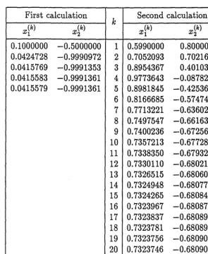
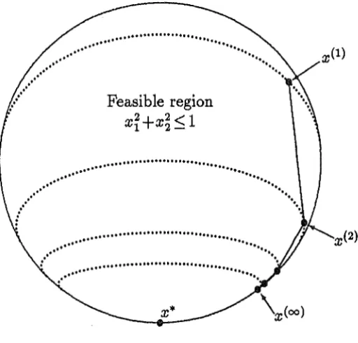
1

Abstract Karmarkar's algorithm for linear programming has become a highly active field of research, because it is claimed to be supremely efficient for the solution of very large calculations, because it has polynomial-time complexity, and because its theoretical properties are interesting. We describe and study the algorithm in the usual way that employs projective transformations and that requires the linear programming problem to be expressed in a standard form, the only inequality constraints being simple bounds on the variables. We then eliminate the dependence on the transformations analytically, which gives the form of the algorithm that can be viewed as a barrier function method from nonlinear programming. In this case the directions of the changes to the variables are solutions of quadratic programming calculations that have no general inequality constraints. By using some of the equalities to eliminate variables, we find a way of applying the algorithm directly to linear program-ming problems in general form. Thus, except for the addition of at most two new variables that make all but one of the constraints homogeneous, there is no need to increase the original number of variables, even when there are very many constraints. We apply this procedure to a two variable problem with an infinite number of constraints that are derived from tangents to the unit circle. We find that convergence occurs to a point that, unfortunately, is not the solution of the calculation. In finite cases, however, our way of treating general linear constraints directly does preserve all the convergence properties of the standard form of Karmarkar's algorithm.

November, 1989

1 _{Department of Applied Mathematics and Theoretical Physics, University of Cambridge,}

1. Introduction

A linear programming problem is the minimization of a linear function of real variables subject to linear constraints on the values of the variables, which may include equality conditions as well as inequalities. We let n be the number of

variables, x E Rn be the vector of variables, cTx be the objective function where c is a constant vector in Rn, and S be the set of points in Rn that satisfy the linear constraints. We assume that S is nonempty and bounded, and, due to linearity, it is a convex polytope. We define a vertex to be a point of S that is on the boundaries of n linearly independent constraints and an

edge to be a straight line segment. in S that is contained in the intersection of

n-l boundaries of linearly independent constraints. Thus the two end points of each edge are vertices. Thinking geometrically, it should be clear that the least value of cTx subject to x ES can always be achieved at a vertex, and that sometimes there are many optimal vectors of variables.

The most widely used algorithm for solving linear programming calcula-tions is the simplex method. The main operacalcula-tions of this algorithm can be viewed as moves from vertex to vertex along edges of the polytope, each edge being chosen so that the move reduces the objective function. Thus cycling does not occur, and termination is a consequence of the finiteness of the total number of vertices. Usually this algorithm is very efficient, but our geometrical interpretation shows that many vertices may have to be visited on the way to the solution even for small values of n. Therefore some iterative algorithms have been developed that adjust x by taking straight line steps within the interior of S, and usually they avoid vertices except in the limit when con-vergence occurs to the required solution. Such algorithms are called "interior point methods".

We address the most successful of these methods, namely Karmarkar's al-gorithm. It hit the front page of the New York Times in 1984 because of the stunning improvements in efficiency over the simplex method that were claimed by the author. Many researchers found these claims unbelievable even after trying the algorithm in practice, but they were unable to refute the claims because many crucial details of the implementation of the algorithm are not given in the original paper (Karmarkar, 1984). This intriguing situ-ation developed into the most active field of study throughout mathematical programming, and now the consensus is that the algorithm is much faster than the simplex method in many calculations when n is very large. In any case the

study this popular subject. After reading about one per cent of all relevant publications in order to grasp the main ideas, I decided to relate these ideas to my knowledge of nonlinear programming instead of perusing more papers, not having enough time for both of these activities, and now I agree with Gill, Murray, Saunders, Tomlin and Wright (1986) that the relations to barrier function methods are of fundamental importance. Thus we derive a version of Karmarkar's algorithm that handles general inequality constraints directly, which is not taken from the papers that I read. Applying this version to a semi-infinite programming problem in only two variables, we find that the algorithm is not always efficient when there are very many constraints.

The paper that was most helpful to my studies is a report by Gonzaga (1988), which he kindly provided when I requested some information on an excellent talk that he presented at the 1989 SIAM meeting on Optimization. It explains very well the geometric properties of Karmarkar's algorithm. A brief introduction to these properties is given by Strang (1987), who emphasises that the projective transformations of the algorithm provide "room to move" when one seeks changes to the variables that reduce the objective function. I learnt several useful technical details from Todd and Burrell (1986) and from Gill et al (1986) which are mentioned later. The other papers that I read are of less relevance to the material that follows, but certainly I would have been helped greatly by the work of Tomlin (1987) and Shanno (1988) if I had chosen to discuss numerical comparisons to the simplex method and modified projections that are easy to compute.

2. The basic algorithm

Throughout Sections 2-4, the feasible region S is the set

(2.1)

where A is a given nxm matrix with linearly independent columns and a0 is a given vector in 'R"'. Because there are only n inequality constraints, this form is not very suitable for the geometric interpretation of Section 1, but in fact ex-pression (2.1) does not lose generality in theory. Indeed, any general inequality constraint,

wT

x

>

bi say, can be expressed as the equation Xi=

wr

x-bi and the simple bound Xi~ 0, where Xi is a new variable of the calculation, so the only

inequalities are nonnegativity conditions on the components of an augmented

x. Further, we can ensure that at most one constraint has a nonzero right han,d side by forming linear combinations of equality constraints if necessary. Alter-natively, the conditions WT x

=

b, for example, can be replaced by WT x-,Bb

=

0 and

/3

= 1, where

/3

is a new nonnegative variable, so all the constraints become homogeneous in the new vector of variables except for

/3

= 1.

It has been mentioned already that we require S to be nonempty and bounded, and that in this case the linear programming problem has at least one solution, x* say. Strengthening this assumption, we suppose that a vector xC1) is available that is in S, that has strictly positive components, and that is

not optimal, which implies the inequality

(2.2)

The notation xC1_{) is used, because Karmarkar's algorithm requires such a point}

in order to begin an iterative procedure that calculates x(kH) from x(k) for k

=

1, 2, 3, .... Our assumptions provide the following fundamental properties of the linear programming problem.

Lemma 1 Let

S

0 be the closed set

(2.3)

Every element of

S

0 satisfies the inequality

(2.4)

where M is the constant

M = max{llxlb

I

xES}.

(2.5)

Proof Because inequality (2.4) is trivial when x

=

O, we let x be a nonzero

element of

S

0 • The value of a'{;x is nonzero, because if we had a'{;x = 0 then

we would also have ( x<1)

+AX)

E S for all ,,\ 2::: O, which would contradict the boundedness of S. Further, a'{;x is positive if x is a multiple of x<1) because

a5x<1> = 1 and both x and x<1) have no negative components. Otherwise, if a'{;x

were negative, then the vector v = x - ( a'{; x) x<1) would be a nonzero element

of

S

0 that satisfied a'{;v

=

0, which is the previous contradiction. Therefore

a'{;x is positive, and, since inequality (2.4) is homogeneous in x, we can restrict attention to the vectors of

8

₀ that are also in S. In this case the bound (2.4) is a consequence of a'{;x = 1 and the definition (2.5), which establishes the first half · . of the lemma. The second half is true because, if x* had no zero components, then the point v = x*

+ ..\(

x<1) - x*) would be in S for some negative values of

..\, giving the contradiction cTv

<

cTx*, while the condition a'{;x*

=

1 does not allow all the components of x* to be zero. 0

We now consider the procedure that calculates x<k+t) from x(k) when x(k)

>

0

and x(k) ES. Several authors, in particular Strang (1987), motivate the

proce-dure by taking the view that, if some of the components of x<k) are very small, then the corresponding nonnegativity conditions cramp the choice of x(k+t), so it becomes difficult to achieve a substantial reduction in the objective function. Therefore we seek a change of variables,

x=T(x)

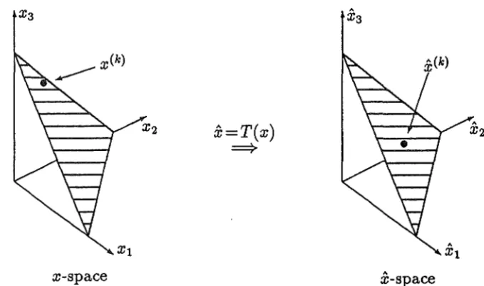
from x-space to x-space say, that maps x(k) and S into 5:(k) and §(k) respectively, such that 5:(k) is not close

to the boundaries of the inequality constraints of §(k). We pick a search

direc-tion J(k) in §(k), and move along it from 5:(k) to i;(k)+a(k)J(k), where a(k) is the step-length of the line search. The new point x(k+t) is obtained by applying an inverse of the transformation to 5:(k)+a<k)J(k).

Of course T depends on x(k), and at first sight the transformation is nonlin-ear, because we require "room to move" about 5:(k) without §(k) being a severe distortion of S when some of the components of x(k) are very small. We let X(k) be the n x n diagonal matrix whose diagonal elements are the (positive) components of x(k), and for each k the transformation is the formula

(2.6)

where e is the vector in nn whose components are all one. The denominator

is positive because every x in S has no negative and at least one positive components. Thus the inequality constraints x ~ 0 become

x

2::: O, and x(k) is mapped into 5:(k)

=

e, which is well away from the inequality constraint boundaries as required. Further, the equality conditions ATx = 0 become the equations ;l(k)T5: = O, where A.(k) is the matrix

X3

x-space

x=T(x)

==>

£-space

Figure 1: A transformation in three dimensions

which depends on the symmetry of X(k). Further, the inhomogeneous condition

a5x

= 1 is irrelevant to

x,

because the transformation (2.6) is independent of the scaling of x, but we see that

x

satisfies

eTx

= n. Therefore 5(k) is the set

(2.8)

We let the inverse transformation be the formula

(2.9)

the denominator being positive because X(k)£ is a nonzero vector in the set (2.3) for all £(k) E S(k). This denominator gives the condition

a5x

= 1. Thus the transformation and its inverse provide a one-to-one correspondence between S and 5(k). In particular, if the only equality constraint is the inhomogeneous equation

X1

+x2+· ·

·+xn

=

n, (2.10)

then a0=e/n and S(k) is the same as S for all k. Figure 1 shows this transfor-mation when n = 3, the feasible regions being shaded.

[image:7.598.100.440.134.335.2]

homogeneous constraint a~x = 1 of expression (2.1) becomes irrelevant, which is appropriate to the homogeneity of the transformation (2.6). Further, we can forget the denominator of formula (2.9), because now only the direction and not the magnitude of x is important. Thus, for each k, there is now a one-to-one correspondence between the half-lines from the origin in the set (2.3) and the points of §(h). In practice the vectors { x(h)

I

k = 1, 2, 3, ... } that occur in the calculation are nonzero points on the appropriate half-lines that need not satisfy the normalization condition arx<h) = 1, but of course the vector of variables that is returned to the user of the algorithm is scaled so that it is in S. Lemma 1 shows that this scaling can always be done.

The technique that admits the objective function {c1'x

I

x E

n.n}

into this structure is an essential ingredient of Karmarkar's algorithm. A "potential function" {V(x)

I

xESo} is employed, where So is the set

So= {x

I

x>O, ATx=O},

(2.11)

which includes all the points { x<h)

I

x

=

1, 2, 3, ... } that have been mentioned. We require V to tend to its least value when the sequence {x(h)

I

k = 1, 2, 3, ... } tends to a solution

x"',

because every iteration provides the reduction

(2.12)

We also require the half-line structure to be preserved, which demands that V(.-\x) be independent of .,\ for all x E S0 , where .,\ is any positive number. Karmarkar's solution is to include the term log c1'x in V(x) and to provide ho-mogeneity by some balancing log Xi terms, where x; is still the i-th component of x. Specifically, the potential function has the value

n

V(x)

=

n logcTx -

I:

logx;, xESo,

i=l

which is constant on each half-line.

(2.13)

A limitation of this choice is that cT x

<

0 is forbidden, so the solution x"' must satisfy cTx•

>

0. Moreover, if cTx• were strictly positive, then, be-cause Lemma 1 shows that x"' has a zero component, the sequence {V(x(h))

I

k = 1, 2, 3, ... } would diverge to +oo if x(h) ~

x"',

which would not allow the decreases (2.12) in the potential function. Therefore we have to make the "restrictive assumption"

Lemma 2 The given assumptions imply that the function (2.13) is well-defined but not bounded below. If { x(k)

I

k = 1, 2, 3, ... } is a sequence of points in So that satisfies condition (2.12), and if the values of the potential function

{V(x(k))

I

k = 1, 2, 3, ... } tend to -oo, then {x(k) / a5x(k)

I

k = 1, 2, 3, ... } is a well-defined sequence in S whose limit points are solutions of the linear

programming problem.

Proof Let x be any point in S0 • Lemma 1 and the definition (2.11) imply that

x/a5x is a well-defined point of S that has positive components. Therefore, by Lemma 1 again, it is not a solution of the linear programming problem, so we have cT(x/a5x)>cTx""'=O. Hence cTx is positive, making the value (2.13)

well-defined. .

Let x(1_{) and x• be a point of So and a solution of the linear programming}

problem respectively, and let 1""' be the set

{i

I

xt

=0}. Therefore

11""'1,

which is the number of zero components of x•, satisfies 11""'

I

<

n. We consider the potential function on the line segment whose end points are x• and x(l). The

"restrictive assumption" and the definition of T imply that, for every O

<

0::; 1, we have the relation

V(x""'+O[x(1>-x•])

<

n{logO+log(cTx(1) ) } - °I:{logO+logxf>}

ieI•

- I:

1og(min[x;, xP>n, (2.15)

i¢I"

which is an inequality rather than an equation only because of the final sum. Since the dependence on O is contained in the term ( n

-11""'

I) log O, the limit

() ~ 0 establishes that V is not bounded below.

Lemma 1 shows that the sequence { x(k) / a5x(k)

I

k

=

1, 2, 3, ... } , given in the statement of Lemma 2, is well-defined, and it is bounded because it is contained in S. Further, we are told that the numbers {V(x(k) /a5xU0_{>) =}

V(x(k))

I

k=l,2,3, ... } tend to -oo. In view of the definition (2.13), it follows that cTx(k) / a5x(k) tends to zero. Therefore, by continuity, all limit points of { x(k) / a5x(k)

I

k = 1, 2, 3, ... } are points of S at which the objective function

is zero. Hence the restrictive assumption implies that these limit points are solutions of the linear programming problem as required. D

We now address the details of the iteration that calculates x(k+l) from x(k)

x = T(X(k) x) when x E S(k), expression (2.13) implies the value

A l'l, l'l, )

V(x) = V(X(k)x) = n logc(k)T5: - I)ogxi - I:logxik, xES(k), (2.16)

i=1 i=l

where c(k) is the vector

(2.17)

The polynomial time result, given in the next section, depends strongly on the fact that, at x

=

x(k)

=

e, the second derivative matrix of the term { -

I:i

log

Xi

I

x

E nn} is the unit matrix. This property makes projected steepest descent methods efficient in x-space. Therefore the search direction J(k) is defined by projecting the negative gradient

- \7\/(e)

= __

n_c(k)

+

e (2.18) c(k)Te

into the set {d

I

A_(k)Td

=

O,

eTd =

O}.

Thus the vector x<k>+aJ(k) remains in 5(k) when a is sufficiently small and positive. Forgetting the constraint eTd = 0 for the moment, but remembering that the columns of A are linearly independent, this procedure gives the vector

J(k)

=

[J -A_(k)(A_(k)TA_(k)tlA.(k)T]

(e _

c(k~Te c(k)).

We were forgetful because we see that the identity

A_(k)Te=ATx(k)e=ATx(k)=o

(2.19)

(2.20)

implies eTJ(k) = 0. Therefore there is no need to include the condition eTd = 0 explicitly in the projection that defines the search direction.

This definition provides the downhill condition

(2.21)

and it will be shown in the next section that the inequality is strict. Therefore the reduction

(2.22)

can be achieved by choosing a(k)

>

0. The advantage of the room to move is

that the feasibility condition (x(k)+a<k)J(k)) E S(k) does not impose a small upper bound on the step-length. We let a(k) be this bound, and we let a(k)

minimize the new value of the potential function {V(x(k)+a J(k))

I

O ~a~ a(k)},

implies that V(x(k+l)) and V(x(k)) have the values V(x(k)+a(k)J(k)) and V(x(k)) respectively.

In view of Lemma 2, we expect the sequence {V(x(/c))

I

k=l,2,3, ... } to tend to

-oo,

which will be proved in Section 3. Therefore the iterations are terminated when the inequality

(2.23)

is obtained, where L is a prescribed constant. This condition and the

defini-tions (2.5) and (2.13) imply the bound

(2.24)

where x(k) is the vector x(k) / a5x(k). Thus the final value of the objective function, namely cTx(k), is at most M e-L, which provides guidance on the choice of L.

When condition (2.23) does not hold, we require the components of x(k) to be positive, in order to calculate x(k+l). The initial vector satisfies xC1₎

>

_{0 by}

hypothesis, and x(k+l) inherits strict positivity from x(k) if a(k)

<

o;(k), where o;(k) is defined soon after expression (2.22). The alternative case a(k) = o;(k) is very unusual, because then the - I:i log Xi term of the potential function (2.16) blows up, so the reduction (2.22) implies that c(k)T(i;(k)+a<k)J(k)) is zero, although all points of §(k), in particular S;(k) +a(k)J(k), are nonzero. It follows by analogy with inequality (2.15). that the new value of the potential function is V(x(k+l)) =lima--.a,. V(x(k)+a J(k))

=

-oo,

which will satisfy the termination condition (2.23) when k is increased by one, the vector x(k+l) / a5x(k+l) being a solution of the linear programming problem. Therefore we have x(k)

>

0 at the beginning of every iteration that has to revise the variables.

3. Convergence properties and the restrictive assumption

curvature of

V

that ensures that the directional derivative remains negative for a substantial distance along the search direction, and (c) that the step-length is not restricted severely by the boundary of an inequality constraint. So far we have given most attention to condition (c), noting that :v(k) = e and that

the inequality constraints are the simple bounds

x

~ 0. Thus, because the def-inition (2.19) takes account of the equality constraints, feasibility is preserved if we impose the bound

(3.1)

on the change of variables in x-space. The reason for the choice of right hand side will become clear.

One comment of Section 2 is highly relevant to condition (b ), namely that at

x

=

5:(k)

=

e the second derivative matrix of the term { - Li log Xi

I

x

ER"'}

of the potential function (2.16) is just the unit matrix. Further, for general x, the second derivative matrix of this function is the expression

-r,2V"(")- n "(k),..(k)T d' (1/"2)

v X - - _(c(k)Tx)2 C c

+

1ag Xi , (3.2)

the last term being the n

x

n diagonal matrix whose diagonal elements have the values { 1 /

x;

I

i = 1, 2, ... , n}. Thus we have the upper bound

(3.3)

when

x

satisfies {xi~

f

I

i = 1, 2, ... , n }. We make use of this relation at the points {

x

= 5:(k)

+

a J(k)

I

a ~ 0}, whose components are all at least

!

when inequality (3.1) is obtained.

In order to show that condition ( a) also holds, we deduce the following conclusion from the restrictive assumption (2.14), using the notation

(3.4)

for the symmetric projection matrix that occurs in the definition (2.19) of the search direction.

Lemma 3 At least one component of p(k)c(k) is nonpositive, where c{k) is

the vector (2.17).

Proof Let x* be a solution of the linear programming problem and, as in Section 2, let X(k) be the diagonal matrix whose diagonal elements are the positive numbers {

x}")

I

i

=

1, 2, ... , n}. The constraint AT x* = 0 and the definitions (2.7) and (3.4) imply

x<")

p(k)

x<k>-

1x* =x*. Thus we can write the final value of the objective function in the form

Now this expression is zero by the restrictive assumption, and, remembering

x* 2::: 0 and the last statement of Lemma 1, the vector X(k)-1_{:v* has no negative}

and at least one positive components. Therefore we would have a contradiction if all the components of p(k)fP~> were positive, so the lemma is true. D

Equations (2.19) and (2.20) imply the value

J(k) - e - _n_p(k) c<k)

- c(k)Te ' (3.6)

and the denominator c(k)Te = c<k)Tx(k)-lx(k) = cTx(k) is positive. Hence we deduce from Lemma 3 that not every component of J(k) is less than one, which provides the bound

(3.7)

It follows from the projection technique that defines J(k) that the initial direc-tional derivative of the line search satisfies the inequality

J<k>Tv1v(x<k>) / 11J<k>112 - -[P<k>vv(x<k>) fvv(x<k>)

I

11J<k>112 = -11p<k>v1v(x<k>)11~

I

11J<k>112

= -11J(k)l'2 ~ -1. (3.8)

Conditions (a), (b) and ( c) that are mentioned in the opening paragraph of this section are expressions (3.8), (3.3) and (3.1) respectively. Therefore it is now straightforward to establish the main convergence property of Karmarkar's algorithm.

Theorem

4

The given assumptions imply that the reduction V(x(k))

-V(x(k+l)) is bounded away from zero on every iteration that calculates x(k+l)

from x(k).

Proof Let {</>(a) I a 2::: 0} and

a

denote the values of the potential function {V(x(k>+a J(k)) I a 2::: _{O} and (2 IIJ(k)ll 2)-}1 _{respectively. From the definition of}

a(k), the Taylor series with explicit remainder and the three conditions that have just been mentioned, we deduce the relation

V(x<k>+a<k>J<k>)

<

o~fa

</>(a)

- o~f)

</>(O)

+

a </>'(O)

+

fo'\a-0) </>"(O) d()]

min_[ V(x(k))

+

a J(k)Tv1V(x(k))

0:50::50:

+

loo: (

a-0) J(k) Tv72\/( £(k)

+ ()

J,(k)) J(k) d()]

<

minJV(x<k>) - a 11J<k>112

+

2a2 11J<k>11~1

(3.9)

the last line being derived from the value a=(4

IIJ(k)ll

2 )-1

=!a,

The theorem

follows from the fact that the reduction in

V

is the same as the reduction in

v.

0

The well-known polynomial-time complexity property of Karmarkar's algo-rithm is a consequence of a corollary of this theorem, namely that the number of iterations that are needed to satisfy the termination condition (2.23) is bounded above by a constant multiple of n.

We now relax the restrictive assumption cT x*

=

0 that is made in Section 2. If the optimal value of the objective function,

c1'

x* = 1* say, is known in advance, but 1* is nonzero, then it is sufficient to modify c before beginning the calculation that is described in Section 2. Specifically, because the definition (2.1) implies that x* minimizes cTx subject to x ES if and only if it minimizes

(c-1*aofx subject to x ES, we can replace c by c-1*a0 in order that the optimal value of the new objective function is zero. Usually, however, 1* is not available. In this case for each k the calculation of x(k+l) from x(k) depends on

an estimate 1(k) of 1*, where 1(1) is given and where the subsequent values are

generated automatically so that the sequence { 1(k)

I

k = 1, 2, 3, ... } converges

to 1*, On the k-th iteration c is replaced by the vector

c(k)

=

c - 1(k) ao, _(3.10)

which induces the new value

(3.11)

of expression (2.17), and corresponding changes are made to equations (2.16), (2.18) and (2.19), but the sets S,

s

0 ,

s(1c>

and So and the transformations

(2.6) and (2.9) are the same as before. Having made these modifications, the procedure of Section 2 generates x(k+l) from x(k), unless it is detected that 1(k)

should be revised.

Of course 1(k) is unacceptable if a negative value of c3(k)Tx occurs during

the line search from £(k) = e along the direction J(k), because then the potential function (2.16) is not properly defined. We see that equations (3.10) and (3.11) give the identity

(3.12)

Moreover, x E s(k) implies X(k)5; E

So

and then Lemma 1 shows that

a5

x(k)x

is positive, x being nonzero because it is in s(k). Therefore we can avoid the

negative value of c3(k)T5; by reducing 1(k). We recommend being generous when

c(k)T5; remains positive throughout the line search, because there is a highly suitable way of making the sequence {,(k)

I k

= j,j + 1,j +2, ... } increase monotonically to ₁*, where j is any integer such that ,(j) ~ ,* (Todd and

Burrell, 1986). This technique depends on the following lemma. Further, the lemma sometimes provides a useful lower bound on the new value of ,(k) when ,(k) is decreased.

Lemma 5 Let x(k) be any vector in S_{0 ,} let .A.(k) and p(k) be the matrices (2.7) and (3.4), where as usual X(k)=diag(xfk)), and let,* be the least value of the original objective function {cTx Ix ES}. Then, if all components of the · vector p(k) c:.<k) are positive, the strict inequality ,(k)

<

₁* is satisfied.

Proof Let x* solve the linear programming problem and suppose that, as in the statement of the lemma, we have p(k)c(k)

>

0. Since x* is nonzero and nonnegative and since x(k) E So implies x<k)

>

O, these conditions give the strict inequality e,(k)T p(k)X(k)-1_x•

>

_{0. Moreover, as in the proof of Lemma 3, the}

equation X(k) p(k)X(k)-1_{x• = x* holds. Therefore the condition c(k)T X(k)-}1_x•

>

O is satisfied, and, remembering expressions (3.10) and (3.11), we write it in the form (c-₁(k)a₀

)T

x*

>

0. The lemma now follows from the definition,* =cTx*

and the constraint a5x* = 1. D

The lemma suggests the useful procedure that will be described in the next paragraph. It requires a lower bound

,<

1_{) on the optimal value of the objective}

function to be given instead of the restrictive assumption cT x" = 0. For each _I in the set { ,(k)

I

k = 1, 2, 3, ... }, the potential function is now the expression

n

V(x;_{1 )}

=

n log[(c-_1aofx]-

I:

log xi, xESo, _{1 ~ 1}*, (3.13)

i=l

which is still homogeneous in x. We see that the case ₁ = ,* corresponds to the potential function that we had before, so Lemma 2 shows that V(x;,*)

is well-defined for all

x

E S0 , the scalar product

(c-

1*a0

)Tx

being positive.

Otherwise, when ₁

<

,*, we apply Lemma 1 to x E S0 C

8

0 in order to deduce the condition

(3.14)

Thus V(x; _{1 )} is still well-defined. Expression (3.14) also provides the inequality

V(x;_{1 )}

>

V(x;,*), xESo,

,<,*,

(3.15)

which will be needed later. We preserve the definition

V(x;

_{1 )} = V(x; _{1 ) when}

The k-th iteration of the revised procedure is supplied with a lower bound

,(k) on

,*,

given by the user when k = 1 and inherited from the previous

it-eration when k

>

1. It is also supplied with a vector of variables x(k) that as

before is in 80 or there is the remote possibility that x(k) has some zero

compo-nents because it is the solution of the linear programming problem, which can happen only if 1<k) =1*, The iterations are terminated if V(x<k>;1(k)) ~ -Ln,

this test being no weaker than condition (2.23) in view of inequality (3.15). When termination does not occur, all components of x<k) are positive, we let

c(k) and c(k) have the values (3.10) and (3.11), and we define the search direc-tion J(k) by formula (2.19). If every component of J(k) is less than one, then it

follows from equation (3.6) and Lemma 5 that we have 1(k)

<

,*.

We seize this opportunity of being able to increase 1(k) in a way that preserves ,(k) ~

,*,

letting the new value of 1(k) be the least larger number such that the vector

p(k)c(k) = p(k)X(k}(c-1<k)a_{0 )} has a zero component. We then return to the beginning of the iteration to retry the termination condition and to recalculate the search direction if necessary. Thus J(k} satisfies condition (3. 7) on every

iteration that changes the variables. As before, x(k+l} is any positive multiple of X(k}(x<k>+a<k)J(k)), where the step-length a(k) is found by a line search that minimizes the potential function. Finally, 1(k+l} is set to the current value of

,(k} and the next iteration is begun.

An important property of this technique for increasing 1(k} is that it guar-antees that Lemma 3 is valid on every iteration. Therefore the deduction in inequality (3.9) and the definition of

V

provide the condition

V(x(k+l}; 1(k})

<

V(x(k}; 1(k}) -

i,

(3.16) where ,(k) has the value that is chosen by the k-th iteration. Increases in ,(k)

also reduce the potential function, because we have noted already that a5x is positive in the definition (3.13). Therefore Theorem 4 applies to the revised algorithm, giving the same polynomial-time complexity property as before. Further, if the termination condition is omitted and if none of the points {x(k}

I

k= 1, 2, 3, ... } is an exact solution of the linear programming problem, then the sequence {V(x(k}; ,(k})

I

k

=

1, 2, 3, ... } must decrease monotonically to -oo. It follows from inequality (3.15) that the sequence {V(x(k};,*)

I

k= 1, 2, 3, ... } also decreases to -oo. Therefore, by Lemma 2, all limit points of { x(k) / a5x(k}

I

k

=

1, 2, 3, ... } are solutions of the linear programming problem as before. Further, the increasing sequence { ,(k)

I

k = 1, 2, 3, ... } tends to

,*,

because, if its limit were

1

<

1*, our deductions since equation (3.13) and the definition (2.5) would imply the inequality

lim V(x<k>;1<k>) - lim V(x<k>/arx<k>;,<k>)

k-+oo k-+oo

>

lim n log [ (

c-1aof x(k) / arx(k)] -

n log M

k-oo

- limn log [

(c-,"'aofx(k) /arx<k)

+ (1"'-1)] - n logM k-oo

- nlog(,"'-1)-nlogM, (3.17)

which contradicts the fact that the sequence {V(x(k);,(k))

I

k = 1,2,3, ... } diverges to -oo.

Thus the main convergence properties of Karmarkar's algorithm are re-tained by the above procedure. In the remainder of the paper, however, we revert to the basic algorithm of Section 2 in order to simplify notation, except that techniques are given in the final paragraphs of Sections 4 and 5 that ex-tend the work of these sections to the case when only a lower bound on the optimal value of the objective function is known initially.

4. Making the transformations implicit

The explicit transformations from x-space to x-space and back again, that occur in every iteration of the algorithm of Section 2, can be avoided by some algebra. It was pointed out by Gill et al (1986) that the resultant algorithm is a "barrier function method", due to the fact that the potential function (2.13) usually becomes infinite if one or more components of x

>

0 tend to zero. The algebra does provide a big simplification, partly because it removes the need to distinguish between x-space and x-space. Therefore this alternative form of Karmarkar's algorithm is derived in this section, in two different ways that are shown to be equivalent. Thus we identify some interesting and useful properties of the new form of the old method.

We begin by considering the choice of step-length of the line search of the algorithm of Section 2, which is defined in the paragraph that includes inequalities (2.21)-(2.22). We recall that o:(k) is the value of o: that minimizes {V(x<k>+o:J(k)

I

O~o:~o:(k)}, and we also recall that we can define

V

by the equation

V(x)

=

v(x<k>x),

(4.1)

as in expression (2.16). Hence, remembering the relation

x(k)

=X(k)e=X(k)£(k) and introducing the search direction

(4.2)

in x-space, the step-length minimizes the function

V(x<k>+o:J<k>) -

v(x<k>[x<k>+o:J(k>])

Having calculated a(k), the procedure of Section 2 sets x(k+i) to any positive multiple of X(k)(£(k)+aJ(k)), which includes the usual choice

(4.4)

Further, the bound a(k) is defined to be the greatest number such that all components of x(k)+a(k)J(k) are nonnegative, which is also the greatest number such that the components of X(k)(x(k)

+

a(k)J(k)) = x(k)

+

a(k)d(k) have this property, since X(k) is diagonal and positive definite. Therefore each iteration of Section 2 that changes the variables can be implemented in the following way. The search direction ( 4.2) is calculated. Then a(k) is found by minimizing the function ( 4.3), the bound a< a(k) being the condition x(k)+a d(k);?:: 0. Finally,

x(k+l) is defined by formula (4.4).

We complete this description by removing the dependence of d(k) on the transformations. Equations ( 4.2), (3.6) and (2.17) and further use of x(k) = x(k)e imply the value

ik) - x(k) - _n_ x(k) p(k) x(k)c

- c1'x(k) ' (4.5)

while the definitions (3.4) and (2.7) yield the matrix

p(k) = I - x(k) A(ATx(k)2At1 ATx(k), _(4.6)

which give the search direction

ik) = x<k) - _n_ [X(k)2 - x(k)2A(ATx(k)2At1 ATX(k)2] c. (4.7) cTx(k)

The calculation is now in a form that has no explicit dependence on £-space. A check on our algebra is that the method of Section 2 was designed to have the property that, if x(k) satisfies the equality constraints AT x(k) = O, then

x(k+l) also satisfies them. In view of formula ( 4.4), an equivalent statement is

that we expect ATd(k) to be zero whenever AT x(k)

=

O, and we see that equation ( 4. 7) passes this test. Another check is that, because we found using equation (2.20) that eT J(k)

=

O, we should now have the identity

(4.8)

Formula ( 4.7) satisfies this condition because of the relations eTX(k)-lx(k) =n, eTX(k) c

=

cT x<k) and eTX(k) A= x(k) TA= 0. We gain further knowledge of d(k) by studying a different way of eliminating the

x

variables from the definition (4.2).

(2.18) the orthogonal projection operator into the null space of A_(k)T. This construction implies that J(k) is the point in the subspace {d

I

A_(k)Td=O} that is closest to -'vV(e), where distance is measured in the Euclidean metric. Therefore the squared distance 11J(k)+'vV(e)lrn is made as small as possible.

In other words, J(k) is the solution of the quadratic programming problem

minimize dT'vV(e) +} lldll~,

subject to A_(k)Td = O

Therefore the solution of the analogous calculation

dE'R" } ,

minimize (X(k)-1_{df'vV(e) +} IIX(k)-}1_dll~,

subject to A_(k)T(X(k)-ld)

=

Q

(4.9)

(4.10)

must occur when X(k)-ld

=

J(k), which is when d is the search direction ( 4.2) in x-space. Since the derivative of the identity ( 4.1) with respect to

x

provides the relation

( 4.11)

and since .A.(k) is the matrix (2.7), it follows that the required search direction

in x-space is the solution of the quadratic programming problem

minimize dT'vV(x(k))

+

!

dT x(k)- 2d,

subject to ATd = 0

dE'R" } , _(4.12)

Again we have a definition of d(k) that does not depend explicitly on the transformations of Section 2.

In order to solve this problem analytically, we let µ(k) be the vector of Lagrange multipliers at its solution. Therefore d(k) and µ(k) satisfy the linear equations

'vV(x(k)) + X(k)-2d(k) = Aµ(k) } .

ATd(k) = 0 (4.13)

Multiplication of the first equation by ATX(k)2, in order that d(k) can be elim-inated by the second equation, yields the vector

(4.14)

By substituting this expression into the first equation, we find the search di-rection

Therefore, since the potential function (2.13) has the gradient

v'V(a/k)) = _n_ c - x(k)-2x(k)

cTx(k) ' (4.16)

where the last term is a convenient form of the vector with components {1/ x~k)

I

i = 1,2, ... ,n}, and since ATx(k) = 0, we see that formulae (4.7) and (4.15) are equivalent. More importantly, the quadratic programming problem (4.12) provides a valid definition of the search direction.

We extend this point of view by considering the second derivative matrix of the potential function, which has the value

v'2_{V(x(k))=- n ccT+X(k)-2 (4.17)}

(cTx(k))2 .

We note that the diagonal matrix X(k)-2 also occurs in expression ( 4.12). Indeed, the work so far of this section has established the following theorem, which provides a description of an iteration of Karmarkar's algorithm that seems to be much clearer than the one that is developed in Section 2.

Theorem 6 Given a point x(k) E 80 , an iteration of the algorithm first tests

the termination condition (2.23). If a further improvement to the vector of variables is required, then the gradient of the potential function (2.13) and the diagonal second derivative matrix of the

-I:

1 log Xi term are calculated at

x

=

x(k). The search direction d(k) is defined to be the solution of the quadratic programming problem ( 4.12). Finally, the new vector of variables is given the value (4.4), where the step-length a(k) minimizes the univariate function {V(x(")+a d(k))

I

a

2::

O}, subject to the condition x(k+l)

>

0. D

The relation to the "log barrier method" for constrained optimization that was noticed by Gill et al (1986) is as follows. We let y(k) be the approximation to the potential function that is formed by replacing the n log cT x term of the definition (2.13) by the first order Taylor series expansion

n log cTx ~ n log cTx(k)

+

_n_ (x-x(k)f c (4.18)

cTx(k) ·

Thus the gradients v'V(x(k)) and v'V(k\x(k)) are equal and the second deriva-tive matrix of expression ( 4.12) is v12

v<"\x<")).

_{Therefore d(k) is the} Newton-Raphson search direction at x(k) of the linearly constrained nonlinear program-ming problem

minimize

{v<"\x)lxE'R.n}

subjectto ATx=O. (4.19)

Lemma 2, however, shows that actually the algorithm solves the problem

since the -

Li

log xi term of V keeps x nonnegative. Perhaps, therefore, we should be considering the Newton-Raphson search direction of this calculation at x(k), which is normally defined to be the solution to the problem ( 4.12) after replacing X(k)-2

=

v'2V(k)(x(k)) by the matrix v'2V(x(k>). Unfortunately this approach is unsuitable, because now the quadratic programming calculation cannot have a unique solution due to the homogeneity of V. Indeed, we suppose that d(k) is a solution and we consider the set of vectors { d = d(k)+ox(k)

I

()En}.

For every() the constraints ATd=O are satisfied due to ATx(k)=O, and the new quadratic objective function

takes the value

Q( d(k)

+

()x(k)) = Q( d(k))

+

()d(k) Tv72y( x(k)) x(k)' ()ER, ( 4.22)

because, by homogeneity, the terms x(k)Tv'V(x(k)) and x(k)Tv'2V(x(k)) x(k) are zero, which is shown explicitly in the derivatives ( 4.16) and ( 4.17). It follows that d(k) is well-defined only if the function ( 4.22) has a unique minimum at

() = 0, which is impossible as the dependence on () is linear. Therefore the use of the function (4.19) instead of the function (4.20) when calculating the search direction by a Newton-Raphson procedure provides some stabilization that is certainly needed if one employs a general numerical method for quadratic programming.

In fact the homogeneity makes the vector x(k) in the definition (4.7) re-dundant. A good way of interpreting this remark is to take the view that is presented in the paragraph that follows equation (2.10), namely that {V(x)

I

x E 80 } is not a function of the point x but instead is a function of the

half-line {,\ x

I ,\

>

O}. Thus the set of points {x(k)

+

a a(k)

I

a

2::

O}

can be regarded as a set of half-lines, and the line search must find the step-length

a(k) that minimizes the constant value of the potential function on the half-line {,\ (x(k) +a(k)d(k))

I ,\

>

O}. Thus only the directions and not the magnitudes

of the vectors {x(k) +ad(k)

I

a ~ O} are important. Further, the positive line search parameter makes all half-lines in the convex hull of the half-lines

{,\ x(k)

I ,\

>

O} and {,\ d(k)

I ,\

>

O} accessible. Now, if we drop the x(k) term from the definition (4.7), the new search direction is d(k)_x(k), and the new line search has access to all half-lines in the convex hull of {,\x(k)

I

,\>0} and

{,\ (d(k)_x(k))

I,\>

O}. Therefore, by taking the average of the new extreme half-lines, we find that the old line search over the range O:::;

a:::;

oo is equiv-alent to the new line search over the range O

<

a :::; 1. Further, the old range 0

<a:::;

a(k) that occurs in equation ( 4.3) becomes the new range O:::;

a:::;

&(k),

of x(k)+a(k)d(k), which gives the value &(k) = a(k)j(l+a(k)). Therefore the deletion of x(k) from expression (4.7) would preserve the choice (4.4), apart from an unimportant scaling factor.

Some use will be made of this freedom in Section 6, but until then we re-tain the usual choice of search direction that we have derived in two different ways. The fact that this choice satisfies equation ( 4.8) provides a noteworthy property. Specifically, since we have X(k)-le = X(k)-2x(k), condition ( 4.8)

implies that the search direction is orthogonal to the last term of the gra-dient (4.16). Therefore there is no first order change to the penalty term

{- Ei

log Xi

I

x E S_{0 }} of the potential function when the step-length of the

line search is small. Because this term is strictly convex for all x E S0 , its second derivative matrix being diag(l/ x;), it follows that every iteration of the algorithm increases the penalty term. Therefore Theorem 4 shows that not only {V(x)

I

xES0 } but also {logcTx

I

xES0 } is reduced by a substantial

amount on every iteration. Although this observation is interesting, it does not illuminate the progress of the variables towards the solution of the original linear programming problem, because we are not taking account of the nor-malization condition a'[x = 1 that is imposed by the inhomogeneous constraint.

Further, it is straightforward to construct examples where the change to the variables gives ~(x(k+l)ja'[x(k+l))

>

c!I'(x(k)ja'[x(k)), although the reduction cT x(k+l)

<

c7

x(k) is guaranteed.

When the restrictive assumption is replaced by a lower bound ,(k) on the final value of the objective function, we recall from the last three paragraphs of Section 3 that we replace c by the vector (3.10) wherever it occurs. Thus formula ( 4. 7) provides the search direction

ik) = x(k) - n x(k)p(k)x(k)(c-,(k)ao),

( c-,(k)ao)T x(k) (4.23)

We also recall that it is advantageous to increase ,(k) if all components of the vector

(4.24)

are positive, the new value being the least larger value of ,(k) that causes a component of this vector to become zero. After any increase the search direction ( 4.23) is recalculated. Thus at least one component of d(k) is no less

than the corresponding component of x(k), which gives the bound

( 4.25)

5. General inequality constraints

In many linear programming problems one has initially far fewer variables than constraints. For example, one may require the cubic polynomial fit to one hundred given measured values of a function of one variable, { (

t

_3,

J;)

I

j = 1, 2, ... , 100} say, that minimizes the maximum residual of the fit. In this case it is convenient to employ five variables, which are the four coefficients of the cubic polynomial and an upper bound on the maximum residual that is going to be made as small as possible. Thus the calculation is expressed in the linear programming form

2 3

-subject to

x1+x2t;+x3t;+x4t;-xs

~

J;

< x1+x2t;+x3tJ+x4tj+xs,

}

, (5.1)

j = 1, 2, ... , 100

where c is the fifth coordinate vector, because we wish to minimize the value of x5 • We see that there are two hundred linear inequality constraints and no

simple bounds. Therefore one might introduce some new variables in order to express the calculation in standard form, some suitable techniques being mentioned in the opening paragraph of Section 2. The standard form, however, has as many variables as inequalities, so in this case the number of variables would increase from five to at least two hundred. We are going to show, therefore, that Karmarkar's algorithm can handle general inequalities directly, avoiding the need to increase the number of variables, except that one extra variable is usually required to make all but one of the constraints homogeneous. Our claim that the standard form of the problem (5.1) requires at least two hundred variables presumes that there is no preliminary calculation that depends on the details of the data, an extreme and unreasonable example of preliminary work being the solution of the problem itself. Assuming that the actual numerical values of the elements of the vectors and matrices that specify the problem are the concern of the main linear programming algorithm, it is not possible to say in advance that any of the inequality constraints are redundant. Therefore, as mentioned already, the number of variables of the standard form is at least the initial number of inequality constraints. Moreover, whenever the standard form demands a new variable, a new equality condition is introduced too, in order that the amount of freedom to change the variables remains the same. Hence it is usual for the equations AT x = 0 in the calculation of Section 2 to have the property that it is easy to employ some of them to eliminate some of the new variables from the standard form, in order that these new variables do not occur explicitly.

of the standard form AT x = 0 have the structure

the components of y and z being the first r and last n - r components of x respectively. Thus, because the total number of equations is still m, the

dimensions of BT and zT are (m+r-n)xr and (n-r)xr respectively. Further, if A does not give the structure (5.2) immediately, we postmultiply it by a nonsingular m x m matrix, U say, that provides the partitioning

AU= (

!

1-: )

(5.3)

in order that expression (5.2) is equivalent to ATx = 0. Such transformations exist for any choice of the integer r from [n-m, n-1], because of the assumption that the homogeneous equality constraints are linearly independent, but the

n-m variables that are expressed in terms of the remaining variables by the identity

z =

zTy cannot always be the last n-m components of x. Therefore we assume that the variables are reordered if necessary.

For any y E 7?/ we form the vector x = x(y) E 'R,n by appending

z

= zTy to

y. It follows that the problem of minimizing {V(x)

I

x E So} is equivalent to minimizing the new potential function

W(y)

=

V(x(y))

= n log

hTy-

t,1ogy, - f.1og

(t,z,m),

yEYo, (5.4)

where h E

nr

is defined by the identity hTy = cTx(y), which gives the compo-nents

n-r

hi= Ci+

I:

Zw;·+j, i= 1, 2, ... , r,

(5.5)

j=l

and where

Yo

is the set {y

I

x(y) E S0 }. Thus, by analogy with

expres-sion (2.11),

Yo

is the set of vectors that provide positive arguments of the logarithms of the potential function (5.4), and that satisfy the relevant ho-mogeneous equality constraints. These constraints are now just the m+r-n

conditions BTy=O, which are empty if r=n-m, because n-r of the original constraints have been used to eliminate the last n-r variables of the standard form of Section 2.

We go back to the standard form, however, in order to consider the search direction ( 4. 7) that is generated in x-space. We recall that AT x(k) = 0 implies

defined at the beginning of the previous paragraph and where y(k) and e(k) are composed of the first r components of x(k) and d(k) respectively. Therefore, in view of the definitions (2.13) and (5.4), searching along d(k) from x(k) to minimize the potential function V is equivalent to searching along e(k) from y(k) to minimize the potential function W. Further, the second search gives the vector

(5.6)

in 7?}, where a(k) is the step-length of equation (4.4), and where y(k+t) E n,r

inherits the first r components of x<k+t).

We now take the view that we are working in y-space, so h, B and Z are available, the objective function is { hTy

I

y E n,r}, the constraints are y 2::: O,

zTy 2::: 0 and BTy

=

O, and the potential function is expression (5.4). We let y(k) E

Yo

C n,r be the initial vector of variables for an iteration of Karmarkar's algorithm. If the usual termination condition, which now has the form

(5.7)

is not satisfied, then we are going to calculate y(k+l) in the way that is suggested in the previous paragraph. Therefore we construct the vectors and matrix

(5.8)

in order that formula ( 4. 7) provides a suitable search direction in x-space. As before, the components of e(k) E n,r are the first r components of d(k).

Then y(k+l) is chosen to be the vector (5.6), where, as mentioned already, the step-length a(k) is the value of a that minimizes the univariate function {W(y(k)

+

a e(k))

I a

2::: O}, subject to the condition that the arguments of the logarithms of the potential function remain nonnegative, which should be satisfied automatically. We note that the constraints AT x

=

0 when A is defined by expression (5.8) are equivalent to the original constraints ATx=O, even if U

is different from the identity matrix in expression (5.3). Further, when these constraints are satisfied, the definitions (5.5) and (5.8) make the new value of

cT x the same as the original one, even if some of the last n- r components of the original c are nonzero. Thus we preserve the property that each reduction in the potential function is bounded away from zero.

It is important to the main result of this section to eliminate from this use of formula ( 4. 7) the explicit dependence on x(k), c, X(k) and A. Indeed, we are going to express the search direction e(k) in terms of h, B, Z and y(k). In theory this can be done by substituting the definitions (5.8) into equation (4.7)

therefore, we take advantage of the fact that we know already that d(k) is the solution of the quadratic programming problem ( 4.12). Fortunately, this derivation of e(k) is easy and highly instructive.

We separate the variables of the problem (4.12) and the matrix X(k) by the partitions

d=

(t)

(

y(k)

and x(k)

=

O

i(k) ) '

(5.9)

where e and fare in 'R/ and

n,n-r,

and where the dimensions of y(k) and n(k)

are r x r and ( n-r) x ( n-r) respectively, so e is no longer the vector of ones. Of course y(k) and O(k) are diagonal matrices whose diagonal elements are the components of the vector x(k) of expression (5.8). We also let Z(·,j) denote the j-th column of Z, which gives the values

n~J)

=

Z(·,J°ly(k), j

=

1, 2, ... , n-r. (5.10)

The definitions (5.8) and (5.9) show that the constraints ATd=O on the vari-ables of the problem ( 4.12) are the equalities

(5.11)

We use the second condition to eliminate

f

from the quadratic objective func-tion of expression ( 4.12), which provides a strictly convex quadratic funcfunc-tion of the variables e. The required search direction e(k) is the vector that minimizes this function subject to BT e = 0.

It follows from equations (5.9), (4.16), (5.8), (5.10) and (5.11) that the linear term of this objective function has the value

dTVV(x(k))

=

_n_ eTh _ eTy(k)-2y(k) _ JTn(k)-2 zTy(k) hTy(k)

n Th Ty(k)-2 (k) ~

Ji

- hT. (k) e - e y - ~ Z(·

')T.

(k)

y 3=1 ,J y

n Th Ty(k)-2 (k) ~ eT Z(·,j)

- hT. (k) e - e y - ~ Z(·

')T.

(k).

y 3=1 ,J y

(5.12)

which gives the good news that the large brackets contain the second derivative matrix of the last two terms of W. We summarise these discoveries by stating that the comment in Section 4 on the calculation (4.19) extends to the current problem. Specifically, e(k) is the Newton-Raphson search direction at y(k) of

the problem

minimize {W(k\y)

I

yEn.r} subject to BTy=O,

where w(k) is the function

n-r

- I: log Z(·,jfy, yE1?t.

j=1

(5.14)

(5.15)

A strong benefit of this technique is that it allows departures from the stan-dard form of Section 2, that provide much useful freedom in the specification of linear programming problems that can be treated directly by Karmarkar's algorithm. It is now convenient not to distinguish between simple bounds and general linear inequality constraints. Therefore we let the original calculation be the problem

minimize h Ty, y E 1?/ }

subject to zTy ~ O, BTy = 0 and b'[y = 1 ' (5.16)

where h and b0 are given vectors in 1?/, and Z and B are given r

x

n and

r x s matrices respectively. This is the standard form when r = n and Z is the identity matrix, but, when Z is rectangular and r

<

n, the standard

form requires some extra variables, which can be eliminated in the way that has been described. Alternatively, the potential function (5.4) anticipates the elimination, and, including any bounds with the general inequalities, it is the expression

n

W(y) = n log hTy - I:log Z(·,jfy, yEYo, (5.17)

j=l

where Yo is the set

(5.18)

Thus the problem can be solved in the following way, that avoids the con-struction of the standard form and occasional large increases in the number of variables.

make the restrictive assumption that the final value of the objective function is zero, but this condition will be replaced by a lower bound on hTy* later,

where y" denotes a solution of the calculation. The k-th iteration in y-space is as follows for the sequence of positive integers k. A nonzero starting point

y(k) is available that satisfies zTy(k) ~ 0 and BTy(k)

=

0. The calculation ends if the termination condition ( 5. 7) is satisfied. Otherwise y(k) is known to be in

the set (5.18) and the vector of variables has to be revised. Therefore we let

e(k) be the solution of the quadratic programming problem

minimize eTv'W(y(k))

+

l eT (~ Z(·,j) Z(·,jf) e

2.

f;;t

[Z(·,j)Ty(k)]2 , eE'R/ } _{, (5.19)}

subject to BTe = 0 the gradient having the value

(k) . n ~ Z(·,j)

v'W(y ) = hT (k) h -

-f--1

Z(.

')T

(k)'

y J=1 ,J y

(5.20)

The new vector of variables is y(k+l)

=

y(k)+a(k) e(k), where, as in the paragraph

that includes equation (5.8), the step-length a(k) is found by a line search that

minimizes {W(y(k)+ae(k))

I

a~O}. Then the next iteration is begun.

However, we have not yet proved that the above algorithm is Karmarkar's algorithm for all the problems (5.16) that satisfy the conditions that have just been stated, because the starting point of the analysis of this section, namely that the equality constraints in x-space can yield the equations (5.2), is not sufficiently general. Indeed, because the elimination that has been described reduces the number of variables, our work so far is restricted to the case when the dimensions of the r x n matrix Z satisfy r

<

n. There is no need for this restriction on the problem (5.16), however, because the boundedness of the feasible region allows more variables than inequalities when there are some equality constraints. Therefore we present a general result that fills this gap.

Theorem 7 Let the problem (5.16) satisfy the conditions that have been stated, and let the sequence of points {y(k)

I

k = 1, 2, 3, ... } be generated by the given algorithm that employs the quadratic programming calculation

(5.19). Then there exists a linear programming problem in standard form,

having n variables and the following property. Defining the sequence { x(k)

I

k = 1, 2, 3, ... } by applying Karmarkar's algorithm to the standard form, these points satisfy the identities { x(k)

=

zTy(k)

I

k = 1, 2, 3, ... }. Further, if x E

n,n

and yE'Rr are any vectors such that x=ZTy and BTy=O, then the potential

function of the standard form has the value V(x) = W(y), where W is the

Proof Let YCR} be the linear space {y

I

BTy=O}. Thus the set of vectors { x = zTy

I

y E

Y}

is a linear subspace of Rn, and we call it S. It is important that the conditions of the theorem imply that the correspondence between

Y

and

S

is one-to-one.

To prove this assertion, we suppose that y(a) and y(b) are different elements of

y

such that zTy(a)

=

zTy(b). Hence the nonzero vector y(c)

=

y(b) -y(a)

satisfies zTy(c) =0 and BTy(c) =0. The condition b'[y(c) /0 must hold, because otherwise the feasible set of expression (5.16) would not be bounded. Further, we let y(d) be the starting vector y<1_{> if y(c) and y(l) are linearly independent,}

but otherwise we let y(d) be a solution y* of the linear programming problem (5.16). It follows that the vector

(5.21)

is nonzero and satisfies zTy(e) ;2: O, BTy(e)

=

0 and b'[y(e)

=

0. Therefore the addition of any positive multiple of y(e) to any feasible vector preserves feasi-bility. In this case, however, the feasible region would not be bounded, so we have a contradiction that gives the required result.

We now choose two matrices z+ and A. The isomorphism that has just been proved and linearity imply that we can let z+ be an n x r matrix that satisfies the equation

(5.22)

Further, we let A be any matrix with linearly independent columns such that

S

is the space { x

I

AT x

=

0}.

Further, we complete the definition of the linear programming problem in standard form, where we are using the notation of Section 2, by setting c = z+h and by letting a₀ be any vector, satisfying the normalization condition

a'[

zTy(1)

=

1, such that the feasible region (2.1) is

bounded. Thus

S

0 in Lemma 1 is {x= zTy

I

y EYo}, where

Yo

is the set

Yo

= { y

I

zTy :2: O, y E

Y }.

(5.23) The two calculations that we are comparing confine the sequences { x(k)

I

k

=

1,2,3, ... } and {y(k)

I

k=l,2,3, ... } to

S

₀ and

Yo

respectively. Further, the isomorphism gives a sequence {y(k)

I

k

=

1, 2, 3, ... } in

Yo

such that {x(k)

=

zTg(k)

I

k=l,2,3, ... }. We have to prove that y(k)=y(k) can be achieved for

all k.

Of course the relation between the potential functions (2.13) and (5.17) depends on the choice c=Z+h. If BTy=O and x=ZTy, then the identity

CTX

=

hTz+T zTy

=

hTy (5.24)

is a consequence of equation (5.22), the condition BTy=O being equivalent to

We begin the calculation of the standard form of Karmarkar's algorithm at the feasible point x(l) = zTy(l), which is in 8₀ because we are given y(l) E

Yo,

Employing the usual notation, we let x(2) = x(l) +ci1_{)d(1), and, because x(2) is}

in

S,

we recall from the isomorphism that x(2) = zTg(2) and g(2) E j) define g(2).

Further, because d(1_{) is in}

S,

_{we can define e<1) by the conditions d(1) = zTe<}1_>

and e(l) E j), which provides the relation

y(

2) =y(1_>+ci1_{>e(l). It follows from the}

equivalence of the potential functions

V

and

W

and the exact line searches that the calculation in y-space gives y(2)

=

jj<

2_{> if and only if the search direction e(l)} is a positive multiple of e(1). In fact we are going to establish e(l) = e(1), and then a straightforward inductive argument completes the proof of the theorem. Therefore it remains to show that x(k) = zTy(k) implies e(k) = e(k).

The search direction d(k) minimizes the objective function of the quadratic programming problem ( 4.12) subject to d(k) ES. Since, for every d ES, there is a unique e E j) such that d = ZTe, and since we have zTe E

8

for every e E j), it follows that d(k) is the vector zTe(k), where e(k) is the valu