Atmospheric physics : electron density variations in the mesosphere

ATMOSPHERIC PHYSICS:

ELECTRON DENSITY VARIATIONS IN THE MESOSPHERE

A thesis presented for the degree of Doctor of Philosophy in Physics in the University of Canterbury,

Christchurch, New Zealand

by D.S. Wratt

ABSTRACT

The theory of the differential absorption and differential phase experiments is examined, and it is found that the

differences in predicted electron densities due to different hypothetical reflection processes are in general no larger than experimental uncertainties.

Results of differential absorption and differential phase measurements are compared.

It is found that electron densities in the mesosphere above Christchurch can be affected by energetic particle precipitation. Evidence is also found for increases in

electron concentration associated with a stratospheric warming, but apart from this there is no clear evidence for

stratosphere-ionosphere coupling above Christchurch.

Model studies show that much of the variation over time scales of four days or more above Christchurch could be

Abstract Notation

CONTENTS

CHAPTER 1: INTRODUCTION

CHAPTER 2: THE THEORY OF THE PARTIAL REFLECTION EXPERIMENT

2.1 2.2 2.3 2.4 2.5

Polarization of the characteristic waves Mode coupling on reflection

Collision frequency irregularities The differential abso�ption experiment The differential phase experiment

2.6 Scattering from a gradual transition in refractive index

2.7 The change of reflection coefficientswith

1

3 6 8 9 14

17

height 23

2.8 The fundamental uncertainty in the Fresnel

model 24

2.9 Summary 26

CHAPTER 3: EXPERIMENTAL DETAILS 28

3.1 Transmitting equipment 29

3.2 The received signals 29

3.3 Receiver 33

3.4 Phase shifting, impedance matching, and

3.5 3.6 3.7

switching

Switching and recording details Experimental procedure

The constraints involved in the various methods

34 36 38

CHAPTER 4: 4.1

Page DATA PROCESSING AND EXPERIMENT UNCERTAINTIES 42

Corrections for noise and criteria for

4.2

accepting data

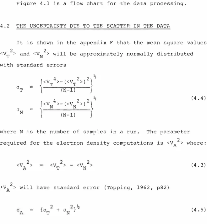
The uncertainty due to the scatter in the data

4.3 Calculation of differential absorption electron densities

4.4 Calculation of differential phase electron densities

4.5 Errors in the differential absorption

42

44

45

47

experiment due to poor impedance matching 48 4.6 Receiver calibration

4.7 Summary of uncertainties 4.8 Day to day variations 4.9 Conclusions

CHAPTER 5: THE DIFFERENTIAL PHASE EXPERIMENT 5.1 Some typical results

5.2 A quantitative comparison between the results of the differential phase and differential

51 52 54 57

58 58

absorption experiments 59

5.3 Conclusions 65

CHAPTER 6: METEOROLOGICAL EFFECTS IN THE MESOSPHERE 67 6.1 Variations from solar control of the

mesosphere 67

6.2 The mean circulation of the stratosphere and mesosphere, waves, and warmings

6.3 Mesospheric observations at the time of stratospheric warmings

70

6. 4 Observations of planetary-scale effects in the lower ionosphere and stratosphere­ ionosphere coupling

6. 5 6.6

Meteorological measurements in the D-region Conclusions

CHAPTER 7: D-REGION ELECTRON DENSITIES OVER BIRDLING'S FLAT

80 84 85

88 7. 1 The seasonal behaviour of electron density 89 7. 2 Diurnal changes in electron density 93 7. 3 _{The winter-spring periods of 1972 and 1973} 97

7. 4 Conclusions 10 8

CHAPTER 8: ELECTRON DENSITY VARIATIONS ASSOCIATED WITH

GEOMAGNETIC STORMS 110

8. 1 Energetic electrons, and the radiation belts

of the Earth 111

8. 2 The solar-terrestrial events of August 1972 113 8. 3 The ionization of the atmosphere by energetic

8. 4 8. 5 8 . 6

electrons

Calculations from the Isis-2 data

Discussion of the production rate results Conclusions

CHAPTER 9: THE THEORY OF ELECTRON DENSITY VARIATIONS IN THE MESOSPHERE

9. 1 9. 2 9. 3 9. 4 9. 5

Production and loss of ionization Nitric oxide transport

The chemistry of nitric oxide

The solution of the nitric oxide equation Electron loss rates

117 123 128 131

9. 6 The results of the model 9.7 Comparison with observations

9.8 The meridional transport of nitric oxide

CHAPTER 10: CONCLUSIONS

APPENDIX A: Electromagnetic Theory

APPEND IX B: Collision frequency profiles

APPENDIX C: The modified magnetoionic theory of Sen and Wyller

APPENDIX D: The rate of change of concentration of an atmospheric constituent in an atmosphere with eddy diffusion, mean �otion, and

photo-APPENDIX E:

APPENDIX F: APPENDIX G:

chemical processes

The absorption suffered by a radio wave totally reflected in the E-region

Uncertainty considerations Switching logic and circuits

Page 162 163 169

172

174 186

188

190

192 195 199 APPENDIX H: Programmes for the software controllec

differential absorption and phase experiment 201 APPENDIX I: Time series of electron densities,

meteorological variables in the stratosphere,

and geomagnetic indices 210

REFERENCES 211

LIST OF FIGURES

Figure Page

2.1 Dependence of differential phase parameters on electron density

2 . 2 2.3 2.4 2. 5 2.6 3.1

The profiles considered by Austin Epstein tanh profile

Epstein sech2 profile

Uncertainty in reflector separation Probability density for t

Hybrid circuit

3.2 Impedance matching from aerial feeders to 75D coax cable

3.3 "Manual" differential absorption equipment

3. 4 Equipment for the "programme controlled" DAE and DPE measurements

3. 5 Procedure for "hardware controlled" differential absorption-phase experiment

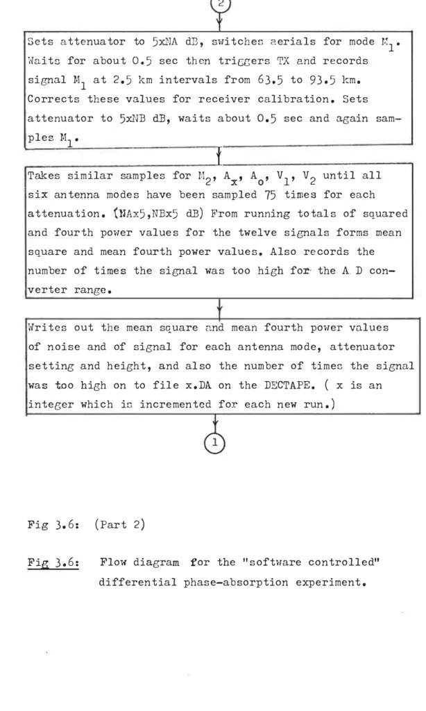
3.6 Flow diagram for the "software controlled" differential phase-absorption experiment 4.1 _{Flow chart for data processing}

5. 1 DAE and DPE electron densities (1416 hours, 13/9/72)

5. 2 DAE and DPE electron densities (1435 hours,

5.3 6.1 6.2

1/8/7 2)

Mean values for DAE and DPE electron densities Absorption at constant solar zenith angle

Latitudinal cross-section of zonal wind speed 6. 3 Typical mean temperature profiles for West

Figure Page 6. 4 Superposed epoch analysis of daily ionospheric

7.1 7.2 7. 3 7. 4 7. 5

absorption index and stratospheric temperature Mean seasonal profiles

Summer and winter profiles

Coefficient of variation (1972) Diurnal variation at 76 km

Diurnal variation at 81 km

7. 6 Electron densities and stratospheric temperatures (13-23rd July, 1972)

7. 7 8.1 8.2

SCR Channel A radiances, July 15 - July 21 1972 Radiation belt morphology

D3E latitude profiles

8. 3 Electron densities, particle fluxes, and magnetic indices for August 1972

8.4 f . for Christchurch and Campbell Island, _min August 1972

8. 5 Lowest altitude of penetration of precipitating electrons

8.6 8.7 8.8

Ionization by energetic electrons - two models Pitch angle distribution at 1400 km

Ion-pair production rate profiles

9 . 1 Ion-pair production rates from various sources of D-region ionization

9 . 2 Photoionization rate of nitric oxide by solar 0

Lyman-a, X = 60

9. 3 Photochemical lifetime of nitric oxide (winter) 9. 4 The effect of 1, 4 and 10 days of vertical motion

on the nitric oxide profile

9.5 The effect of 1, 4 and 10 days of vertical motion on the electron density

75 92 92 92 92 92 107 107 112 112 112 112 118 122 125 127 135

14 3 135

16 3

Figure

Electron density ratios

Partial reflection of a radio wave Volume scatter geometry

9.7 Al A2

A3 The reference height in the volume scatter theory El Electron density profile used in absorption

calculations

Gl Station control register

G2 Circuit to gate SCR bits into switching logic G3 Relay switching

G4 Circuit to set up operations sequence in the "hardware controlled" method

GS Logic for receiving aerial switching G6 Aerial lead switching

G7 Reversing and manual attenuator switching GB Switching logic for the programme controlled

attenuator

G9 Programme controlled attenuator GlO Attenuator circuits

Il Magnetic index (IK) for Arnberley, Winter 1972 I2 Nimbus IV S.C.R.: Channel A, 1972

I3 I4 I5 I6 I7 I8-Il5

Daily temperature Daily temperature Daily height for Daily height for Daily zonal winds

Daily electron

for 20 rnb surface, for 30 rnb surface, 30 mb surface, 1972 100 rnb surface, 1972

at 25 km, 1972 densities, 197 2 Il6-I22 Daily electron densities, 1973.

1972 1972

Page 163 175 175 175

194 200

Table 2.1

LIST OF TABLES

Polarization of the characteristic waves

2.2 Coupling coefficients for reflection at a sharp boundary

2.3 Differences between volume scatter and simple

Page 6

8

Fresnel electron densities from DAE measurements 13 2.4 Difference between volume scattering and simple

Fresnel electron densities for differential phase 16 2.5 Differences in predicted electron density between

the Epstein tanh profile and the Fresnel discon-tinuity model

2.6 Differences in predicted electron density between the Epstein sech2 profile and the Fresnel

discontinuity model

4.1 True values of extraordinary to ordinary ratios for given measured values

4.2 Possible errors in the DAE experiment (1972) due to changes in receiver characteristics

4.3 Uncertainties in differential absorption electron densities for one run.

4.4 Uncertainties in differential phase electron densities for one run

4.5 5.1 5.2 7.1 7.2 7.3

Daily and seasonal variation of electron density DAE and DPE data for 1420 hours, 13/9/72

Comparison analysis of DAE and DPE results Seasonal statistics for electron densities Variation in electron density by season Correlation analysis for 76 km

21

22

51

52

52

53 56 58 60 91 93

Table

7.4 Ionospheric drifts for July-Sept 1972

7.5 Zonal wind above Christchurch as predicted by the thermal wind equation and measured by ionospheric drifts

8.1 8.2

Pitch angle distribution

Electron fluxes for various pitch angles

8.3 Production rates for the 8-particle fluxes of energy greater than 150 KeV

9. 1

9.2 9.3 9.4

9.5 9.6 9.7 9. 8 9.9

Reactions involving nitrogen constituents Lifetime of NO under various reactions Lifetime of N0₂ under various reactions Lifetime of N(4_{s) under various reactions}

Lifetime of N(2D)

Production of odd nitrogen from nitrous oxide Relative concentrations of N0₂ and NO (daytime) Production of odd nitrogen from N₂

Relative concentrations of N(2_{D) and NO}

9. 10 2.4 MHz absorption for the Mechtly and Shirke profiles

Bl Mean seasonal pressure data

Page 103

105 126

127

128 143 146 14 7 148 149 151 152 154 155

NOTATION

The more important symbols are listed here, together with the sections in which they are defined.

a B B

C

E

F (h)

f

Extraordinary mode signal Ordinary mode signal

radius of the earth

magnetic field flux density

( 3. 2)

( 3. 2)

rate coefficient for "attachment-like" loss ( 9 • 5) ( 2 • 2)

coupling coefficients for reflection speed of light

electric field strength (Appencix A) electric field of ordinary, extraordinary

wave (Appendix A)

initial electron energy

electron density difference for two models pulsewidth-dependent term

( 8 • 3)

(2,4,2.5)

( 2 • 5)

magnitude of complex correlation Coriolis parameter

incident electron flux

(Appendix A)

( 7 • 3)

( 8 • 3)

g acceleration of gravity

h height

H scale height

i

_{X y} ,f ,i _Z unit vectors to east, north, vertical.

j

m imaginary part of

k

K

K

(= w/c) propagation constant in free space (App. A)

magnetic index (7. 3)

eddy viscosity (App. D)

L L N e N N p p p p_{j_} Q (fl R R r s T u u w X y

electron loss rate Mcllwain parameter

signal obtained by adding east-west and north-south signals in phase

( 9 • 1)

( 8 • 1)

( 3. 2)

signal obtained by shifting east-west phase by

0

180 and adding it to north-south signal electron density

electron density

complex refractice indices

number of measurements in sample parameter calculated in D.P.E. ion-pair production rate

pressure

momentum normal to magnetic field parameter calculated in D.P.E. reflection coefficient

Fresnel reflection coefficient electron range

correlation coefficient sample standard deviation temperature

parameter in Epstein theory velocity to east

signal from east-west aerial pair signal from north-south aerial pair energy to form one ion-pair

vertical velocity 2 2

w₀ /w w/wL Y cos 8

( 3. 2)

(App. A) (Chapter 4)

( 3. 2)

( 9 • 1)

( 8 • 1)

( 3. 2)

(App. A) (App. A)

( 8. 3) ( 5. 2) ( 4 • 8)

(App. A)

( 7. 3)

( 3 • 2)

( 3. 2) ( 8 • 3) ( 9 • 2)

z

et

et

B

B (h)

e

K

A

]J

]J

v,v _m

p (h)

p p 0 0 T T T

V _m /w (App. E)

2 V m/ W (App . E )

phase of Fresnel reflection coefficient (App. A)

pitch angle (8.1)

electron-ion recombination coefficient (9.5) effective recombination coefficient (9.5) angle between geomagnetic field and vertical (8.3)

Arg(Rx) - Arg(Ro) (App. A)

permittivity of free space

argument of complex correlation (App. A) angle between geomagnetic field and vertical (2.6)

absorption coefficient (App. A)

negative ion to electron ratio (9.5) normalized energy dissipation function (8.3) Mcllwain parameter (invariant latitude) (8.1) real part of refractive index (2.5)

population mean (4.8)

"effective" collision frequency (App. B)

complex correlation (App. A)

wave polarization (App. A)

density

cross-section

Epstein layer parameter pulsewidth

photochemical lifetime optical depth

initial phase of wave geographic latitude geomagnetic latitude

( 9 . 3)

( 2 • 6)

(App. A)

( 9 • 1) ( 9 • 3)

(App. A)

Z 5

X

X

w

>

*

solar zenith angle

imaginary part of refractive index solid angle

angular frequency of earth angular frequency of wave gyrofrequency

plasma frequency

average of a number of measurements (e. g.

x)

unit vector

concentration complex conjugate

( 4 • 8)

(App. A)

( 8 • 4)

( 7 • 3)

1

CHAPTER 1

INTRODUCTION

In the beginning the aim of this worY was to look for

meteorological effects on the electron density in the D-region. The D-region is the part of the ionosphere between about 60 and 90 kilometers above the surface of the earth. The effect of meteorological changes in the stratosphere and mesosphere on the electron concentration in the D-region has been an area of research interest during the last twenty years. It was felt that automated daily measurements of the electron

densities together with measurement of mesospheric winds would make a worthwhile research project, particularly now that

routine temperature information for the upper stratosphere is available from remote measurements by satellite.

However, the discovery of large changes in electron density at the time of a large solar-terrestrial disturbance in August 1972 led to the broader aim of examination of

fluctuations in the electron density in the D-region at middle latitudes and their causes.

The electron densities were measured using the

Thus the work described in this thesis falls into the following categories:

(a) An examination of the theories of the differential phase and differential absorption experiments.

(b) A description of the practical details of the design and operation of the apparatus, the processing of the data, and a consideration of the experimental uncertainties.

2

(c) Tests of the agreement between the electron densities calculated from the differential absorption data and those calculated from the differential phase results.

(d) A review of the literature for evidence and theories on meteorological effects on D-region electron densities, and stratosphere-mesosphere coupling.

(e) A comparison of variations in the electron densities measured in the D-region during the winter-spring period of 1972 with variations in meteorological variables in the stratosphere and mesosphere.

(f) An investigation of the diurnal variation of electron densities in the light of photochemical models.

(g) Consideration of the effect of energetic particle precipitation on D-region electron densities at middle latitudes.

(h) The development of a computer model of the photo­ chemistry and transport of nitric oxide, to predict changes in electron density associated with vertical motion. These

CHAPTER 2

THE THEORY OF THE PARTIAL REFLECTION EXPERIMENT

The partial reflection experiment is a method of calculating electron densities in the D-region of the ionosphere. A radio wave pulse is transmitted and the

amplitude at the ground of the waves reflected from various levels in the atmosphere is measured.

3

There have been two approaches to the theory of the

experiment. The first approach historically was that used by Gardner and Pawsey (19 53), Belrose and Burke (1964), and the majority of investigators since then. It assumes that the ionosphere is horizontally stratified, and the reflections observed in the partial reflection experiment arise from plane discontinuities in electron density. This approach may be termed the Fresnel model.

The second approach was proposed by Flood (1968). It has been used in the experiments of those associated with Flood

(von Biel et al. , 1970). This is known as the volume

scattering model. It assumes that the reflections are due to

fluctuations in permittivity in the scattering volume (the entire volume over which the presence of scatterers will give a reflected signal at the receiver at a given time). These fluctuations are assumed to have a time constant long with

4

There has been some dispute over the relative merits of the two models (Holt 1969, Flood 19 69 ) . An experiment which can differentiate between the two to everyone's satisfaction does not appear to have been designed. Von Biel (1971) has offered some good experimental evidence for the volume

scattering case. However, Austin and Manson (1969 ) give

evidence for a localized reflector model (that is, the Fresnel case)

It will be shown that, to the benefit of the experimenter, the electron densities deduced using either model agree very well within the uncertainties introduced by the experimental techniques. In the limit of short pulsewidths the expressions deduced for electron densities from both models agree exactly.

The approach taken here (see appendix A) is to consider one or several Fresnel reflectors, which over the period of the experiment spend equal times in all parts of the

scattering volume. From the point of average power returned during the duration of the experiment this approach is

equivalent to the volume scatter approach, and gives some insight into the agreement between the two models.

In the actual reduction of ex perimental data the formula arising from the Fresnel method is usually used (Belrose 19 70) as it is much simpler to apply than the volume scatter formula.

Another possibility is that reflections do not come from sharp discontinuities in refractive index, but from regions of more gradual change. In this case a full wave solution of the differential equations governing the propagation must be

5

There has been one further change to the theory since the time of Gardner and Pawsey. This involves the use of

refractive indices obtained from the generalized magnetoionic theory (e.g. Sen & Wyller, 1960) . This theory, which is more clearly explained in a paper by Budden (1965) assumes that the collision frequency between electrons and neutral molecules is proportional to the square of the velocity of the electrons

(Phelps and Pack, 195 9 ) . The older Appleton-Hartree formula (Budden, 19 61) assumed that the collision frequency was

directly proportional to the electron velocity. A summary of the Sen and Wyller formulae is given in appendix C.

2.1 POLARIZATION OF THF. CHARACTERISTIC WAVES

If the magnetic field of the earth were vertical then vertically propagating ordinary and extraordinary waves would both be circularly polarized. However, in the usual case, when the field is not vertical, the polarization of the waves is in general elliptical.

The polarizations of the vertically propagating ordinary and extraordinary waves for a typical electron density profile above Christchurch were calculated using the Sen-Wyller theory, and are given in table 2.1. Equation C4 (appendix C) was

used. The calculations were for a 2.4 MHz wave. At

0

Height (km) N _e

65

70

75 80 85 90

-3 Polarization

(cm )

Ordinary

100 1.00j - l.58xlo-5

100 l.OOj - 3.57xl0-5 200 1.00j - 9.85xlo-5 400 l.OOj - l.64 xlO -4 700 0.999j-l.43Xl0-4

1000 0.999j-8.07Xl0-5

N is the electron density _e

Extraordinary -l.00j-l.58Xl0 -l.00j-3.57Xl0 -1. OOj-9. 95x10 -1. OOj-1. 64Xl0 -l.00j-l.4 3Xl0 -l.00j-8.09Xl0

Table 2.1 Polarization of the characteristic waves.

6

-5

-5

-5 -4 -4 -5

The polarization p is defined as the ratio of the y

component of the electric field in the wave to the x component, where the z direction is vertically upwards and the

geomagnetic field is in the x-z plane.

From table 2.1 both characteristic waves may be considered to be circularly polarized in the D-region.

2.2 MODE COUPLING ON REFLECTION

The mode coupling problem is that on a partial reflection of say the ordinary wave, a small amount of extraordinary wave might be generated. This situation can be examined for the case of a reflection from a plane discontinuity of electron density by requiring that the tangential components of electric field intensity and magnetic field intensity should be

were solved by computer for the same frequency, and the same electron density and collision frequency profiles as used for table 2.1. The results, shown in table 2.2, are for a ratio of electron density below to above the boundary of 0. 90. However, the values were the same to within 1% for values of 0.99, 0. 90 and 0.50 for this ratio.

7

The notation used is as follows. Suppose an ordinary mode wave, with electric field EciI) is incident on the boundary

from below. Then let EciR) be the electric field of the ordinary part of the reflected wave, and E�R) be the extra­ ordinary part (the coupling echo). Define the reflection coefficients,

_�oo,

_R

₀

_x

_by:

=

_!lox

=

dlXX and RXO are defined similarly, for the case of an incident extraordinary wave. Define the coupling coefficients COX' CXO by:

=

ldtoxJ

IR.oo

=

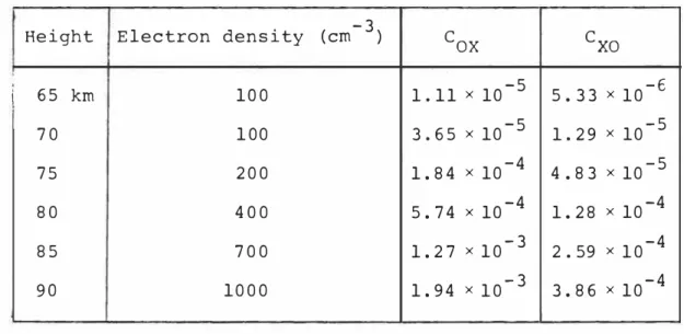
Connolly and Tanenbaum (1972b) have considered a more general case than the plane discontinuity. They calculated coupling coefficients assuming that changes in electron density take place over a significant fraction of a wavelength. The first order coupled equations of Clemmow and Heading were used. For

-5

a wave frequency of 2. 5 MHz, magnetic field of 5xlO tesla,

4 -3 5 -1

electron density 10 cm , collision frequency 10 sec

(roughly equivalent to 90 km over Birdling's Flat) they found that:

8

=

A coupling coefficient of 3 x 10-3 is equivalent to a

factor of about 50 db in power, while 1 x 10-2 is equivalent to a factor cf 40 db. Since the equipment used was only

sensitive down to about 30 db difference between ordinary and extraordinary waves, mode coupling on reflection can be

neglected.

Height Electron density ( cm ) -3

cox

cxo

i

65 km 100 1.11 X 10-5 5. 33 X 10-t 1.29 X 10-5

70 100 3.65 X 10-5

75 200 1. 84 X 10-4 4. 83 X 10-5

80 400 5. 74 X 10-4 1. 28 X 10-4

85 700 1. 27 X 10-3 2.59 X 10-4

90 1000 1. 94 X 10-3 3. 86 X 10-4

Table 2. 2 Coupling coefficients for reflection at a sharp boundary.

2. 3 COLLISION FREQUENCY IRREGULARITIES

Since the refractive index in the D-region depends on the collision frequency v as well as the electron density N, it is possible that changes in collision frequency could contribute to the reflection coefficients. This possibility is discussed by Gregory and Manson (1969a). Suppose the changes in

collision frequency and electron density are �v and 6N

respectively across Thrane (1966) found

the reflecting boundary. Then Piggot and 6\J/\J

that for a =

6.N/N < 0.2, the reflection coefficient ratio RX/R0 is very close to that for a = 0.

Gregory and Manson argue that for realistic processes in the D-region a< 0.2 does hold.

9

The assumption that the reflection coefficient ratio does not depend on 6\J/\J is made in the present work.

2.4 THE DIFFERENTIAL ABSORPTION EXPERIMENT

2.4.1 The Basic Equation

It is shown in appendix A (equations A30, A31) that:

I Exl

= B

_{1/R,x I}

exp (-2I:

Kx

dz) 4h

IEol

= _4h B

l�ol

exp (-2f: K_{0 dz)}

( 2 • 1)

( 2 • 2)

where EX, E0 are the electric fields at the receiving aerials of ordinary and extraordinary waves reflected from a height h. Thus

= _{( 2 • 3)}

2

<

I Eo I

> = ( 2. 4)

where the brackets denote averaging over the period of the experiment. It has been assumed that the reflection

10

Suppose there are reflections from heights h and h+6h. Then:

<1 Ex(h+6h)

I

2>

2 <

I�

(h+6h) 1

2_>

<

ldsc

(h) 12>

fh fh+6h

<exp(-4

0Kxdz) exp(-4 h Kxdz) > =

<

I

Ex (h)

I

> _{<exp(-4f K dz) >}

0 X

( 2 • 5)

Making the assumption that the absorption from h to h+6h is statistically independent of the integrated absorption up to h,

<

I

Ex (h+6h)

I

2>

<

I

Ex (h)

I

₂ >

= <

I�

(h+6h) 1 2_>

X

<liR (h) l_X 2> f h+6h

<exp(-4 K dz) > h X

The approximation is now made that

Jh+6h Kx dz

h =

( 2 • 6)

( 2 • 7)

where KX denotes the height average of KX over the interval 6h. Take natural logarithms and let the operator 6 denote the difference between a value at (h+6h) and at h. Then

= _6£n<ldt 1 2> + £n<exp(-4K 6h) >

X X ( 2. 8)

If it is assumed that the electron density and collision frequency stay constant over the period of the experiment KX will be constant and

£n<exp(-4K 6h) > _X

=

11

Similarly,

Thus

< I E 1_X 2>

= _{( 2. 9)}

__ T_o obtain electron density, (KX-KO) is replaced by (KX-KO_N J-N. Thus

N

=

- 6£n <IE 1

2 > X

< I E 1

2

>

0 _{( 2 .10)}

2.4.2 The differences between the results obtained from the volume scattering and the simple Fresnel models* It is shown in appendix A (equation A27) that Flood's volume scattering theory leads to the expression:

=

= Rx

2

(sinh (CtKX) l

R ₀ 2 ctKX

Thus for this model, as the pulsewidth t tends to zero,

-+ R X 2 R 2 0

(2.11)

which is the value obtained for the simple Fresnel model of a single plane discontinuity.

12

To find the difference likely in the calculated electron densities for the experiment (pulsewidth T = 25 microseconds) between using the volume scatter reflection coefficients and the simple Fresnel ones calculations were made for a typical electron density profile (approximately the average profile found by the DAE experiment over Christchurch for winter 1973). The difference for a given set of experimental results will be

E = (2.12)

Calculations for a 2. 4 MHz wave were made for 6h = 5 km and collision frequency profiles as in appendix B. The results are given in table 3.3.

Another possibility is that the reflection for one

height could be from a simple Fresnel discontinuity, while the reflection for another height is due to volume scattering. This case is considered under the "mixed" heading in table 3.3

(6h = _{5 km)}

In a typical experimental run the uncertainties due just to the random scatter of data (300 samples over ten minutes) are at least 5%. The average daily fractional uncertainty in

mean

theAelectron densities, worked out from about four runs daily near noon for winter 1973 was at least 19% for all heights

( table 4 . 5) ,

13

throughout the scattering volume) it appears that the differences between the volume scatter and simple Fresnel

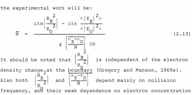
formulae are unimportant experimentally. The equation used in the experimental work will be:

N

=

<IE 1_X 2>

6£n ₂

<jE I > ₀

(Kx-K01_J

4 _N 6h

(2. 13)

R 2 It should be noted that 1

R x

2

1 is independent of the electron

density change2at the boun8ary (Gregory and Manson, 1969a) . Also both

1:x

₂

1

and

(

K

x:

K

o]

depend mainly on collision

frequency, an9 their weak dependence on electron concentration can easily be allowed for by iteration.

Height (km) 65. 0 67. 5 70. 0 72. 5 75. 0 77.5 80. 0 82.5 85.0 87. 5 90. 0

N _e Difference (E) f Difference

-3

(cm ) Absolute Percent .Absolute 100 100 100 140 200 280 400 520 700 830 1000

+2 cm -3 2% l

I

+2

+6 . 4%

!

+8

+11 4% +22

+11 2% -35

+38 5% -49

N is the electron density _e -3 cm (mixed) Percent 2% 6% 8% -7% -6%

Table 2. 3 Differences between volume scatter and simple Fresnel electron densities from DAE measurements.

I I - I

-

-I

I

-I

~

I

_I

I

2.5 THE DIFFERENTIAL PHASE E XPERIMENT

2. 5.l The Basic Equation

It is shown in appendix A (equation A40) that for a volume scattering model the complex correlation

p(h) =

has argument

n (h) =

where

<E E *> _{X 0}

2

2 t:

(<jE I ><IE I >) 2

X 0

14

( 2 • 14)

( 2. 15)

s ( h) = R X, O Fresnel coefficients

�X'�O are the initial phases of the ordinary and extra­ ordinary waves, which are assumed to have the same initial amplitude.

µX,µO are the real parts of the refractive indices. ! (h) is a term involving the pulsewidth T.

e (h) = Arg

(k (nx-n0) c, 1

sin

l---J

k (nx-n0)c, ( 2. 16)

Suppose the complex correlation is measured at two heights h1 and h2. Then

(2.17)

15

As an approximation put:

= _(2.18)

and put

= _(2.19)

Thus

N = (2.20)

2k

l�J

llh

Some trial computations involving the Sen-Wyller refractive R

indices showed that B = Arg (�) is independent of the RO

electron density change across the boundary. Also both Band

� are only weakly dependent on electron density,

depending mainly on collision frequency. Figure 2.1, for 80 km, is typical.

2.5.2 The difference between the volume scatter and simple Fresnel formulae

The difference due to the effect of the finite pulsewidth will be:

E =

2k

[µx�µo]

6h

This was computed for the same profile as used in table 2.3, for llh = 5 km, 1 = 25 microseconds, frequency= 2.4 MHz.

tiB-tin+tie

16

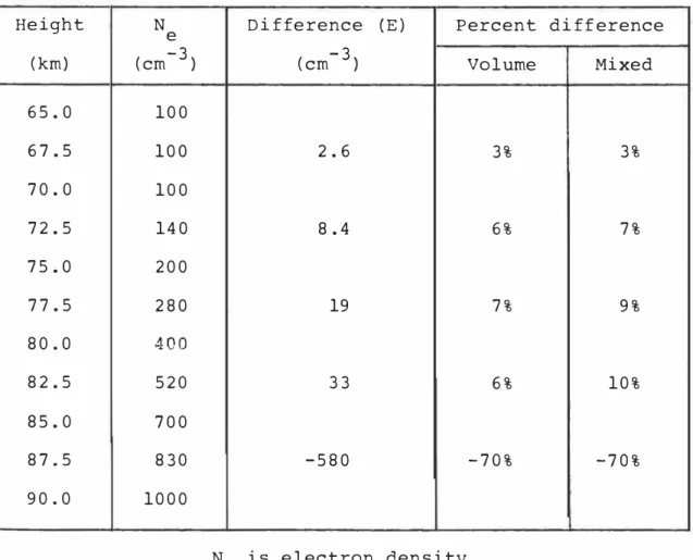
Table 2.4 gives this as an absolute value and a percentage (under the "volume" column) . The column headed "mixed" is the percentage difference from the Fresnel case if there is volume scatter from the upper height but Fresnel reflection at the lower height.

The uncertainty in differential phase electron density for an experimental run (75 independent samples over ten minutes) due to the scatter of the data is usually at least 30%. Thus the differences between the two formulae are unimportant experimentally below about 85 km.

Height N _e

(km) (cm ) -3

65.0 100

67.5 100

70.0 100

72.5 140

75.0 200

77.5 280

80.0 400

82.5 520

85.0 700

87. 5 830

90.0 1000

Difference (E) Percent -3

(cm )

2.6

8.4

19

33

-580

N is electron density _e

Volume

3%

6%

7%

6%

-70%

difference Mixed

3%

7%

9%

10%

-70%

_...

u

'-'

-�z

___...

1.45

l.LJ4

1.43

Or� ( �:)

200 400 600 800 1000

Electron density (cm-3)

Fig 2.1 Dependence of differential phase parameters on

electron density. (80 km, f=2.4 r.:hz )

Height

(refractive index)2

Fig 2.2 The profiles considered by Austin (1966)

.25

·-"'t,

.._,, .24

---��

'-J

.23 ,...

1/l

'

0

o-> \..

2 n

2 --- -- - -

-n2

�__,,...,,:;-::_::- :_I < +

-i< L I )I

I I

Height

Fie 2.3 Epstein tanh profile.

Fi� 2 n

2 nl

2.4

Heieht Epstein sech

L1

I

2

profile.

z

z

2 2

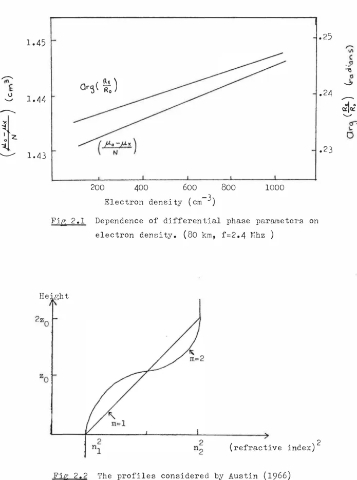
tanh profile: The rnnge L for (n -n1) to go from 10 � to 90% of its final value is 1=

4.38cr-2 2 2)

sech profile: ,The range L over which (n - n1 of its value at the peak is L=

5.00-is more than 10,i \

-...,.-,-..,....,-~

I

-,-17

2.6 SCATTERING FROM A GRADUAL TRANSITION IN REFRACTIVE INDEX

The scattering model discussed so far has depended on

discontinuities in electron density (i.e. changes in electron density over a distance small with respect to a wavelength) ,

so that the W.K.B. approximation could be used right up to the

discontinuity from both sides , and matched across the

discontinuity ,

Connolly and Tanenbaum (1972a) and Austin (1966) have considered the case of a more gradual change in refractive

index . In these cases a full wave solution for the

differential equations governing the propagation of radio waves must be used.

Austin (1966) uses a method due to Millington (1965) to get a full wave solution to the equation

d2E 2 2 + k0 n E

� = 0

for profiles of the form (figure 2.2)

2 2

n = _nl Z < 0

2 o zm

= _{nl +}

2z0 m

2 <5(2Z-Z) = _n2

2Z0 m 2

= _n2

where <5 is a constant.

(2.22)

(2.23)

Austin draws plots of a factor F which modifies the Fresnel

n2-nl

value of R = --- as a function of A , the thickness of the n2+n1 '

18

{fl == FR

There is no discussion on whether F actually depends on n1 and n2. If it does depend on these F will differ for the ordinary

.

lix

and extraordinary modes, and the ratio

IC

wi ll di ffer from the Fresnel value.

Austin also considers reflection from a layer of the form :

and 2 n

2 n

== _{1 + 8}

== 1

. m sin

elsewhere.

}

(2.24)

Here Austin finds that

l�I

== j R j F where R is the Fresnel reflection coefficient , and F is a purely geometrical factor. In this case the ratio of the reflection coef ficients for 0 and X modes will be the same as the ratio in the simple Fresnel case. However , in his derivation Austin obtains F in the form

where the fi ' s are purely geometrical functions. He assumes that this series for F will converge for 8 sufficiently small, and truncates it to F = f0 • Thus the fact that F is a purely geometrical factor is assumed in the derivation and not

proven. Hence the comment of Austin and Manson (1969) that the ef fect of a gradual change in refractive index is "to reduce the reflection coefficient by a geometrical factor

which is equivalent for ordinary and extraordinary modes" must be taken as not proven.

To investigate this effect on the electron densities calculated from experimental results the approach of Connolly and Tanenbaum (1972a) of considering partial reflections from

v

19

an Epstein profile was followed . The Epstein theory (see appendix A) gives a full wave solution for the equation

= ₀

for profiles of refractive index n ( Z) of the form :

2

n = _{u =}

z

_a

(2 . 25)

(2 . 26)

Several assumptions are involved in using this theory for the case of an ionosphere with a magnetic field present.

( 1) It is assumed that in the region of interest there is no coupling between extraordinary and ordinary waves. That is, if an ordinary wave only is incident on the region, so that its electric field at the base of the region satisfies

= 0 ,

then the electric field will satisfy that equation throughout the region (and similarly for an extraordinary wave) .

(2) It is assumed that the collision frequency is constant throughout the layer.

Two types of profile were considered : (a) The Epstein tanh Profile (figure 2.3)

2

n = u = -_a

z

(A4 5)

It is assumed that a given electron density distribution gives rise to both ordinary and extraordinary profiles of this same type. This can be shown to be true for the Appleton­ Hartree quasi-longitudinal case, since

+ u eu 2 { ( n2 -nl ) (e +l)+E:3} ,· 2 2 u (e +l)

20

2 ₁ X 2 ₁ X

no =

-

_nx =

1 - iZ + _{YL 1 - iZ - Y L}

2 (Budden 1961)

N e

where X = e

z

\) _YL w

e

2 =

-

= cos

£ 0Inul w WL

N _e electron density, m electron mass , \) collision frequency, wL gyrofrequency, 8 angle between earth's field and the vertical.

Thus

2 2

(nx -nx ) _{2 ·1} =

(2. 27) So that if the collision frequency v , and hence Z is constant throughout the layer,

implies

It was shown earlier in this section (see table 2. 1) that propagation over Birdling ' s Flat is quasi-longitudinal. Thus

_cR

the ratio of reflection coefficients is given by 1/,X from ₀

equation A . 46.

The maximum error due to assuming Fresnel reflection coefficients when the actual reflections are from an Epstein profile will occur when the lower reflection is from a simple Fresnel discontinuity and the upper reflection is from an Epstein profile. This error is shown in table 2. 5 , for

=

=

2 eu 2 2

no +~~(no-no )

2 1

reflecting regions 5 km apart and winter collision frequencies for a 2.4 MHz wave.

Difference

�eight Electron density

(km) (cm ) -3 Ampl itude measurements Phase measurements -3

Absolute (cm ) Percent Absolute (cm ) -3 Percent

65 . 0 100

67 . 5 100 -0 . 1 -0 . 1 % - 3 - 3%

70 . 0 100

7 2 . 5 140 1 0 . 7% - 3 -2%

75 . 0 200

77 . 5 280 3 1% -7 -3%

80 . 0 400

82 . 5 520 26 5% -10 -2%

8 5 . 0 700

87 . 5 830 90 1 1% -10 -1%

90. 0 1000

Table 2 . 5 Dif ferences in predicted electron dens ity between the Epstein tanh profile and the Fresnel discontinuity model .

RX

(R

It was found that_l'.RX was identical to the Fresnel ratio 0

RO for small values

disparity between (Jl

llf';

x increased the values

of a, but there was an increasing RX

and R as a increased. However, as a ₀ of �0 and /RX decreased. In the

calculatiorn the largest value of a which gave a value of both

'°

_d

_'°

_{t than 1}

_o-

_{6 ( M t 1 19 6 9 ) d}

�X an in-_{0 grea er} anson e a ., was use .

(b) The Epstein sech2 Profile (figure 2.4)

This refractive index profile is :

22

2

n

=

_{n1 + n3 -n1 sec} 2 < 2 2) h2 c..£) ₂₀ (A. 4 7)

A similar approach to that used for the tanh profile was followed to find the possible difference from the simple Fresnel model. For a difference of 10% in electron density between the peak and the base it was found that a < 40 m for reasonable reflection coefficients

L

corresponds to -_\ < 1 4

.

.

Height Electron density

-6

( II?- I > 1 o ) •

Difference

-3 Ampl itude measurements Phase

(km) (cm )

This

measurements -3

Absolute (cm . ) . Percent Absolute (cm ) Percent -3

65 . 0 100

67 . 5 100 0 . 5 0 . 5% -3 - 3%

70 . 0 100

7 2 . 5 140 5 4 % -4 -3%

75 . 0 200

77 . 5 280 16 6% -6 -2%

80 . 0 400

82 . 5 520 50 10% - 3 -1%

8 5 . 0 700

87 . 5 830 155 19% -2 -0 . 2%

90 . 0 1000

Table 2 . 6 Differences in predicted electron density between the Epstein

23

The differences shown in tables 2. 5 and 2. 6 are the

maximum likely for this effect , and will be smaller for smaller values of characteristic length o. Thus up to about 85 km the differences between the Fresnel and the Epstein tanh and sech2 models in terms of predicted electron densities from the same experimental data could be about the same as or slightly larger than the uncertainties due to the random scatter of the data.

2. 7 THE CHANGE OF REFLECTION COEFFICIENTS WITH HEIGHT

In the derivation of the volume scattering formulae (appendix A) it was assumed that the Fresnel reflection coefficients RX, R0 were constant throughout the scattering volume. Coyne and Belrose (1973) discuss a model which allows for variations in the reflection coefficients within the

scattering volume.

Their analysis of the experimental data involves

deconvolving the observed reflection ratio curve to obtain a curve which would result from a very short pulse. Their analysis of one example , when there was a valley in the

electron density profile showed that the simple theory (using the observed reflection ratio curve ) badly overestimated the electron density in the valley region when a 50 microsecond transmitter pulse was used.

However , the error could be significantly less for 25

microsecond pulses. Part of the error in the simple theory is due to the neglect of the differential absorption within the scattering volume (the difference given by equation 2. 12)

2 4

2 5 microsecond pulse (c; = 4 km) is much better than that of

a 50 microsecond pulse (8 km) .

The deconvolution process used by Coyne and Belrose was

rather involved, and for 25 microsecond pulses would probably

require height sampling at closer intervals than 2. 5 km. There

was insufficient time to make such an analysis of the

Birdling ' s Flat results. It is realized that the partial reflection experiment analysis used in this thesis will not

pick up details of structure finer than the resolution allowed

by the pulsewidth. However, deep valleys in electron density

profiles do not appear very frequently in rocket probe

measurements (e. g . Mechtly et al. , 1972a) , so errors as large

as those suggested by Coyne and Belrose are not likely to occur very often.

2. 8 THE FUNDAMENTAL UNCERTAINTY IN THE FRESNE L MODEL

in the automatic data collection method which is used

here for the partial reflection experiments, the receiver

output is sampled at time intervals corresponding to 2. 5 km

intervals in height . Assume that a received signal for a

given sampling channel has arisen from only one discrete plane

irregularity . Then there is an uncertainty in the height of

this irregularity of ± c; where T is the pulsewidth of the transmitted pulse, since the reflections received at a given

tiree may have returned from anywhere within the scattering

volume. (A receiver bandwidth which is too narrow will lead

In the calculation o f electron densities by equations ( 2 . 13 ) and ( 2 . 2 1) data from channel s 5 km apart was used .

Thus , for T = 2 5 microseconds (c; = 1 . 8 km) this uncertainty

could mean an error of up to 7 2% in 6h and thus in e lectron

dens ity .

2 5

The si tuation wi l l not general ly be quite this bad

however . In the absence of any other information it must be

assumed that the height from which a re flection comes is

equally l ikely to be any he ight within the scattering volume .

The si tuation is as in figure 2 . 5 . In the experimental case

d = 5 k C T _{= 1 . 8 k}

m , a = 4 m. The probabil ity dens ity function

for £ , the distance between the two reflectors will be as in

figure 2 . 6 . From this figure it can be seen that there is a

7 5 % probabil ity that £ lies between (d-a) and (d+a) . Thus a is a good measure of the error likely to arise . In the

experimental case the percentage uncertainty � x _d 100 from this

source i s 36% .

Note that this source o f uncertainty di sappears entirely

if a volume scattering model is applicable , and it wil l be

cons iderably reduced if reflections come from several heights

within the scattering vol ume over the period of a given

experimental run .

Also , i f the simple Fresnel model is the appropri ate one , scal ing the experimental values from the receiver trace at the

amplitude peaks rather than at fixed interval s could reduce

a

;mcr refl ector / / / / / ,

1//I//I////// II.

I I t l / / 1 I

I

I

F ie 2.5: Uncertainty in reflector separation.

pa )

( d-2a) ( d-a) d ( d+a) ( d+2a)

Fie; 2 . 6: Probabil i ty densi ty for ,l .

Scatterinc vol­ ume for upper sarnplinc channel

Scattering vol­ ume for lower sampling channel

- - - 1

1

2.9 SUMMARY

26

The main difference between the use of volume scatter and simple Fresnel models in calculating electron densities from partial reflection data is an uncertainty in the latter model because of the uncertainty in the position of the hypothetical reflecting layers. In the experiment used at Birdling's Flat this uncertainty in electron density is about 35%. Other differences in the electron density predictions of the two models are less than, or of the order of, the uncertainty due to the scatter in the experimental results below about 8 5 km.

If reflections arise from a gradual transition in refractive index rather than a sharp discontinuity the

differential absorption electron densities based on the simple Fresnel model could be too low by a factor ranging from 0. 1% to 10% for 6 7.5 to 8 2.5 km . The error in electron density predictions from differential phase measurements due to this effect is less than 3% over the same height range.

The equations used to calculate electron densities will be:

Differential Absorption:

N

R 2

6£n

I=½"/ -

6£n

RO

�

4

l y:r=-J

Differential Phase:

N =

(2. 13)

( 2 . 14 )

=

Llh

68 - Lin

2 7

2 2

< ! Ex ! > , < ! E0 ! > and n are measured experimentally , at 2. 5 km intervals fixed by the equipment .

28

CHAPTER 3

EXPERIMENTAL DETAILS

To determine electron densities by the dif ferential absorption method the amplitudes of the ord inary and extra­ ordinary radio wave reflections from various heights are

required. For differential phase electron density calculations the difference in phase between the ordinary and extraordinary reflections is needed. This chapter describes the methods used to measure these quantities.

The phase difference between the two modes has been

measured in two ways. One method is to measure the difference between the phases of the ord inary and extraordinary

reflections from a given height directly (Austin 1971). A variation on this method is to measure the instantaneous phases of the ordinary and extraordinary modes to obtain the dif ference (Belrose et al. , 197 2b). The other method was first suggested and used by von Biel et al. (1970) and involves the measurement of the complex correlation p (h)

(section 2. 5. 1) between the ordinary and extraord inary reflections. This was the method used in the present work.

(It has also been used recently by Wiersma and Sechrist (197 2) . )

3. 1 TRANSMITTING EQUIPMENT

The transmitter at Birdling ' s Flat has the following characteristics :

2.40 MHz 100 kW

29

Frequency Peak power

Pulsewidth Variable, from a minimum of about 5 microsec.

For these measurements 25 microsec. was used. The transmitter feeds a broadside array of four in-phase pairs of half-wave folded dipoles. The dipole pairs run

East-West. The calculated gain of this array relative to an isotropic radiator is 14 db.

3 . 2 THE RECEIVED SIGNALS

The receiving array comprises four half-wave folded

dipoles arranged in a square . The feeders from the two north­ south dipoles are taken to the center of the square where they are connected in parallel and fed to the receiving hut. The east-west pair is treated similarly. Each aerial pair has a calculated gain of 8 db relative to an isotropic radiator .

Consider an orthogonal coordinate system ( x , y , z ) with 2 vertically upwards , x to the east (that is parallel to the transmitting array dipoles) , 9 to the north. The electric field of a radio wave of angular frequency w transmitted from the transmitter array can thus be expressed as :

}1;T = a ;,.. e .. J·wt = a (x+ jy) j wt + (x-j£) j wt 2 e a 2 e ( 3 . 1)

30

and an extraordinary ( p

=

-j) wave, which can be considered to

propagate independently in the D-region.

The field at the receiving aerials, reflected back from the ionosphere can thus be written as the sum of an . ordinary and an extraordinary wave :

E = E E

]

r_J

( x+ j y ) +

J

( x- j y ) ej w t ( 3 . 2 )

where the subscripts O and X refer to ordinary and extra­

ordinary respectively. E0 and E X are functions of time (i. e. of the height from which the transmitter pulse is being

reflected) , which contain both amplitude and phase parts. The signal from the east-west aerials will te proportion­ al to the x component of (3. 2) , i . e .

V j wt 1 e

and the signal from the north-south pair is :

where

V j wt 2 e =

B is a constant.

1

EO

=

B72 [ V l - jV 2 J

1

E X

=

B72 [V 1 + jV 2 J

From

=

=

( 3 . 3 ) and ( 3 , 4 ) I

1

71B

1

-m

• TI

J

-[V l +V 2e _{2 J}

• TI J

-[V1+v2e 2 J

( 3 . 3 )

( 3 . 4 )

( 3 . 5 )

( 3 . 6 )

Thus the amplitude of the ordinary mode signal can be found (to within a multiplicative constant) by phase-shifting

31

the signal from the north-south antenna by 90°, add ing it to the signal from the east-west antenna, and putting the

resultant signal through an amplitude detector. The extra­ ordinary signal amplitude can be obtained similarly, but with a -90° shift of the north-south signal. Denoting the outputs from the detector for these two signals as I Ax l , I A0 1 res­ pectively gives :

<

I

E _X

I

2>

₌

< I A 1_X 2>

The complex correlation coefficient is defined as :

p = <E E *> X 0

( 3 . 7 )

( 2 . 1 4 )

Let M1ej w t be the signal obtained by adding the signals from the east-west and north-south aerials in phase.

Thus

=

( 3 . 8 )

Let M₂ej wt be the signal obtained by shi ftina the phase

of the east-west signal by 18 0° and adding it to the north­ south signal.

M₂

=

₇₂ B _{{ (Eo +Ex)} - j (Eo-Ex) > ( 3. 9)

Thus _{< I M1 l} 2_{> + < I M2 I >} 2

=

2R2 (< I E0 1 2> + < 1 Ex l 2>) (3. 10)

< I M 1₁ 2> - < I M₂

I

2 >

=

-2 jB2 (<ExEo*> - <Ex*Eo>) ( 3. 11)

also < I V1 ! 2

> + < l v2! 2

>

=

B2 (< 1 Eo l 2> + < 1 Ex l 2>) (3 . 12)

<I

E

12>

< I V I 2> - < I V 1 2

I

2>

=

B2 (<E E *> + <E *E >) X O O X

32

(3.13)

Define two new variables P and Q :

p

Q

< l v11 2>-<l v2 1 2> <1Axl 2>+<IA01 2>

< I v 1 I 2> +< I v 2 1 2 > • ( < I Ax I 2 > < I A0 I 2 >)

½

=

<E E *>+<E *E > _{X O O X}

(3 . 14)

(3. 1 5) Then (2.14) can be written as:

p

=

� + . Q _{2 J 2} (3. 16)

But by definition P and Q are both real. Thus if the complex correlation is written as:

p = I P I e in then

I P I cos n =

IP I sin n =

Hence

I P I sin n =

I P I cos n

Thus measuring

p

2

Q

2

k [< I M112>-< I M21 2

> ]

2 _{2 2}

< I M1 I >+<I M2 I >

[< I V1 i 2

>-< I V2 i 2

> ]

½ _{2 2}

<IV 1 I >+< I V 2 I >

(3. 17)

(3. 18)

(3 . 19)

[<IA 1 2

>+< 1 A 1 2>

l

{< l �0 12><1 A: 12>)½

[ < I A I 2 >+ < I A I 2

>

0 X

t< I A 1₀ 2>< 1 A 1_X 2>)½

(3.20)

l

(3. 2 1) the roean squared values for six different signals gives the information required for calculating

<IM1!2>-<IM2i2> <IAxl2>+<IAol2>

< I M

1 I

2

> +< I M

2 I

2

>. ( <

I

Ax I 2 > < I A

0 1

2

33

electron densities from the differential absorption experiment (via 3. 7) and the differential phase experiment (3. 20 , 3. 21) .

3.3 RECEIVER

Two different receivers were used. The first receiver, which was used until July 1973 , was valve operated apart from a silicon diode in the detector circuit . A new solid state receiver developed by J. de Voil in the electronic workshop was used in August and September of 1973 . The characteristics of the two receivers were as follows:

First receiver:

Frequency: 2.40 MHz Bandwidth: 100 KHz

Sensitivity: Minimum discernable signal 0. 1 uV Voltage gain: 85 db

Maximum output: 1 volt

New receiver: Frequency: Bandwidth: Sensitivity: Voltage gain: Dynamic range: Maximum output:

2.40 MHz 65 KHz

Minimum discernable signal 0. 1 uv 90 db

A

\

"A" input

_

L_

--JT

· I �---""'

"A-jB" output

L

L

"13" input

__

L _

"V2

>---� I·

"A+ jB" output

C = 2140 pF

Fig 3 . 1 : Hybrid circu i t .

H _I D

1460 pF 0-9 , 600 pF

2 wire feeder

from

I aerial s

'

0-9600 pF I nl n2

11 . 2 ?H

Transfo1·ner : 34 turns

n2 = 17 turns Li tz wire on Philli ps po t-core.

Fir;ure 3 . 2 : Impcdo,nce matching from aerial feeder::; to

7 5 .n.. coax cable .

I

I • I

-l

c

l.v'

34

3. 4 PHASE SHIFTING, IMPEDANCE MATCHIN� AND SWITCHING

3. 4.l Signal Combination and Phase Shifting

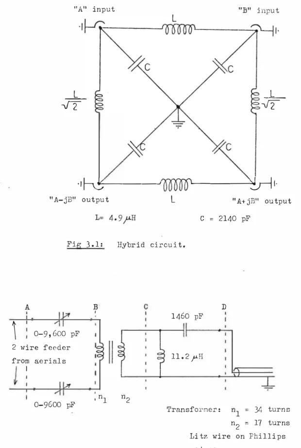
The phase shift of 90° in the signal from the north-south aerial and addition to the signal from the east-west aerial required to obtain the ordinary and extraordinary mode signals was made using a hybrid circuit designed and built by Dr H. A. von Biel (figure 3.1) . It is important that the input and output impedances to this circuit be close to 75D. In practice the A-iB output of the hybrid was permanently terminated in 75 ohms and both the ordinary and the extra­ ordinary modes obtained from the A+iB output by inverting the signal to the B input on alternate cycles (Figure G7) .

To obtain the signals

v

_{1 and}

v

₂ the hybrid was bypassed and the leads from the required pair of aerials were switched directly to the receiver.

To obtain the signal M1 the signals v1 and v2 were added directly across the receiver input. The signal M₂ was

obtained by adding

v

_{1 to}

-v

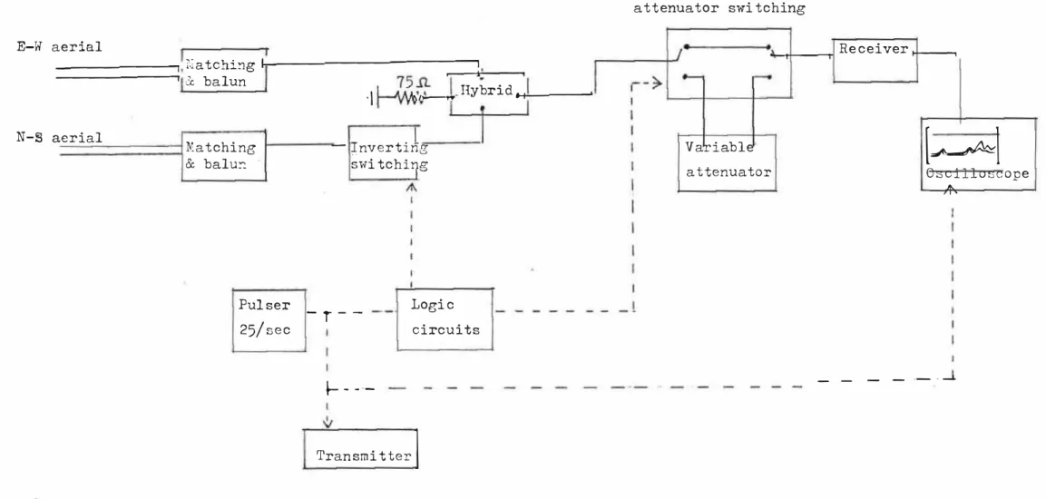
₂ across the receiver input. All of the switching was done by reed relays, as described in appendix G.

3 . 4.2 Impedance Matching

The feeders from the receiving aerials to the receiver hut are balanced open wire transmission lines . The nominal impedance looking back down one of these feeders from the receiver hut is 600 ohms, although in practice the impedance varies from this due to incorrect spacing of the feeders and errors in the impedance matching at the aerials. However, the transmission line used between pieces of apparatus in the