Capacity Analysis for MIMO Two-Hop
Amplify-and-Forward Relaying Systems with the
Source to Destination Link
Abdulla Firag
‡Peter J. Smith
‡Matthew R. McKay
†‡Dept. of Electrical and Computer Engineering, University of Canterbury, Christchurch, New Zealand
†Dept. of Electronic and Computer Engineering, Hong Kong University of Science and Technology, Hong Kong
Abstract—This paper presents an ergodic capacity analysis of an amplify-and-forward multiple-input, multiple-output two-hop system including the source to destination (direct) link. We first derive an expression for the probability density function of an unordered eigenvalue of the system. Then, using this result, a closed form expression for the ergodic capacity of the system is derived. The ergodic capacity expression has one integral that needs to be evaluated numerically. The results produced are valid for all SNR values and for arbitrary numbers of antennas at the source, relay and destination. We also present simulation results to validate our analysis. The results show that the analysis exactly matches the simulations and quantifies the improvements in capacity due to the diversity offered by the direct link.
I. INTRODUCTION
Wireless relaying networks have recently been given con-siderable attention due to their many advantages. Apart from increasing the range, relaying networks can also achieve better diversity by using cooperative transmission from the source and several relays [1], [2]. The relaying terminals forward the information from the source to the destination mainly using two well known methods: amplify-and-forward (AF) and decode-and-forward (DF). In AF mode, the relay terminal does not decode or demodulate, but amplifies the received observations, corresponding to the signal from the source, and retransmits to the destination. Since input, multiple-output (MIMO) systems can provide better system capacity than single-input, single-output (SISO) systems, relaying has recently been extended to MIMO scenarios [3], [4]. MIMO relays aim to provide improved system capacity, increases in range, and better diversity.
In this paper, we analyse the ergodic capacity of an AF MIMO two-hop system including the direct link. Most of the capacity results on two-hop MIMO relays were derived by employing asymptotic methods [5], [6], [7]. Furthermore, the random matrix results required for the MIMO relay capacity analysis are usually presented for two separate cases [8], [9] depending on whether the system is defined by a Wishart or a Pseudo-Wishart [10] distribution. However, a unified expression for the capacity of the AF MIMO two-hop system, without the source to destination link, was derived in [11].
The work of M. R. McKay was supported by Grant RPC07/08.EG16.
Our main contribution in this paper is to derive an exact expression for the capacity of an AF MIMO two-hop system including the source to destination link as shown in Fig. 1. Our expression is unified and it can be used for arbitrary numbers of antennas at the source, relay and destination. We also present simulation results to validate our analysis and the results are used to quantify the capacity improvement due to the direct link.
II. SYSTEMMODEL
We use the relay network topology shown in Fig. 1. The source (S), relay (R), and destination (D) terminals are equipped with ns, nr and nd antennas respectively. During
the first hop, S transmits (broadcasts) to R and D and in
the second hop R transmits the amplified signal from the
first hop to D. We let the normalized channel matrices for
the source-to-relay (S→R), source-to-destination (S→D), and relay-to-destination (R→D) links be given by H1∈ Cnr×ns, H3 ∈ Cnd×ns, and H2 ∈ Cnd×nr, respectively. We assume
that S and R have no channel state information and that
D has perfect knowledge of all channels. In addition, all
channels are assumed to exhibit independent and identically-distributed (i.i.d.) flat Rayleigh fading, and as such, the entries of the corresponding channel matrices are modeled as i.i.d. zero mean circularly symmetric complex Gaussian (ZMCSCG) random variables with unit variance. Furthermore, we assume thatRassists in the communication withDusing AF relaying.
Hence,Ramplifies the received observation corresponding to
the signal fromS by a factor,b, and retransmits it toD. The received signal at the destination after the two hops is then given by
y=
√
P3H3
√
P2√P1bH2H1
x+
n3
√
P2bH2n1+n2
. (1)
In (1), the parametersP1, P2 andP3 are the average powers of theS→R,R→D andS→D links, respectively, taking into account the different path loss and shadowing effects over the links. The variablesn1,n2andn3are the noise vectors atR,
D (second-hop) and D (first-hop) respectively, and x is the
vector of transmit symbols. The transmit symbols are assumed i.i.d. withE{xx†}=ρIns. The noise atRandDis modeled as ZMCSCG with E{n1n†1} =σ12Inr, E{n2n
†
S
R
[image:2.612.52.301.221.321.2]D
Fig. 1. MIMO relay network topology.
and E{n3n†3}=σ32Ind. With this information, and defining
F1=√P2√P1b,F2=√P2b,F3=√P3, the received signal at the destination can also be written as
y=Hx+Bv (2)
where
H=
F3H3 F1H2H1
, (3)
B=
σ32Ind 0
0 σ12F22H2H†2+σ22Ind
1/2
, (4)
andvis a normalized zero mean Gaussian noise vector, which
has I2nd as covariance matrix.
III. CAPACITYANALYSIS
The ergodic capacity of the system is given by [3] as below, (the factor 1/2 accounts for the fact that information is conveyed to the destination terminal over two time slots [1])
C= 12E
log2I2nd+ρHH
†(BB†)−1. (5)
The singular value decomposition of H2 can be defined as
H2=UDV†, where Dis an nd×nr diagonal matrix with
{√ν1, . . . ,√νl} as the main diagonal elements in decreasing
order and where l = min(nd, nr). Then, using the identity
det(I+AB) =det(I+BA)and substitutingH2=UDV† into (5), the ergodic capacity can also be written as
C=12E
log2Ins+ρU
† tAUt
(6)
where A=
σ−2
3 F32Ind 0
0 Ω
andUt=
U†H 3 V†H1
, with
Ω=F12D† σ21F22DD†+σ22I
−1
D. Note thatUtcontains
i.i.d ZMCSCG entries since the unitary matrices U† andV†
do not change the statistics ofH3andH1. After definingc= σ3−2F32,c1= (F12−σ−32F32σ12F22),c2=σ3−2F32σ22,c3=F12, c4=σ12F22, andc5=σ22,Ω can be given as
Ω= ⎧ ⎪ ⎪ ⎪ ⎨ ⎪ ⎪ ⎪ ⎩
diag
c3ν1
c4ν1+c5, . . . ,
c3νl
c4νl+c5
nrnd
diag ⎧ ⎨
⎩c4cν31ν+1c5, . . . ,
c3νl
c4νl+c5,0 , . . . ,0
nr−nd
⎫ ⎬
⎭ nr> nd
.
(7)
Further, by defining m=max(nd, nr), q=nd+l ands =
min(ns, q), the ergodic capacity can also be expressed as
C= 12E
log2Ins+ρU
† tAUt
(8)
where Ut ∈ Cns×q has i.i.d ZMCSCG entries with unit
variance and
A=
cInd 0
0 diag
c3ν1
c4ν1+c5, . . . ,
c3νl
c4νl+c5
. (9)
Note that A and Ut are re-sized versions of A and Ut
according tonr nd or nr> nd. Now the ergodic capacity
can be written as
C= s
2ln(2)
∞
0 ln(1 +ρλ)f(λ)dλ, (10)
whereλdenotes an arbitrary eigenvalue ofU†tAUtandf(λ)
is the probability density function (p.d.f.) of λ. Hence, to find the ergodic capacity of the system, we need to find the arbitrary eigenvalue density, f(λ), of the random matrix
U†tAUt. The derivation off(λ)is given below.
If we assume the random diagonal matrixA has all distinct eigenvaluesμ={μ1, . . . , μq}, then the conditional unordered
eigenvalue p.d.f.f(λ|μ)for arbitrary numbers of antennas at the source, relay and destination can be obtained from [11] as
f(λ|μ) = 1
sqk<p(μp−μk) q
k=q−s+1
λns−q+k−1
Γ(ns−q+k)|G|,
(11)
where Gis aq×qmatrix with entries
Gi,j=
μij−1 i=k
μq−ns−1
j e
−λ
μj i=k . (12)
However, the eigenvalues ofA are not all distinct but can be given as{c, . . . , c, μ1, . . . , μl}, wherecis a constant which has
multiplicitynd, andμk= c4cν3kν+kc5 are random variables which
are unequal with probability 1. When A does not have all
distinct values, the conditional p.d.f. f(λ|μ)can be obtained by using the following identities on multiple derivatives,
1) Ify=xn, then thekth derivative ofy,y(k)= (n−k+ 1)kxn−k, where(n)k is the Pochhammer symbol.
2) If y = xne−s/x, then the kth derivative of y, y(k) = e−s/xk
i=0 i!(kk−!i)!(n−k+ 1)k−isixn−k−i.
These derivatives are then used to derive a modified version of (11) using the method given in [12]. With this approach f(λ|μ)can be calculated as
f(λ|μ) = 1
slk<p(μk−μp)
l
k=1(c−μk)nd
nd−1
k=1 k!
.(−1)q1(q−1)/2
q
k=q−s+1
λns−q+k−1
Γ(ns−q+k)|G|,
(13)
where Γm(n) =
m
Gi,j=
⎧ ⎪ ⎪ ⎪ ⎪ ⎨ ⎪ ⎪ ⎪ ⎪ ⎩
(i−nd+j)nd−jci−nd+j−1 i=k, j= 1, . . . , nd
nd−j
t=0 e−
λ
c (nd−j)!
t!(nd−j−t)!(q−ns−nd+j)nd−j−tλ
tcq−ns−nd+j−1−t i=k, j= 1, . . . , nd
μij−−1nd i=k, j=nd+ 1, . . . , q
μq−ns−1
j−nd e
− λ
μj−nd i=k, j=n
d+ 1, . . . , q
. (14)
we can derive the arbitrary eigenvalue p.d.f., f(λ), as given below. Here we focus onP1=P3, (c1= 0) which is of more physical interest. The special case, P1 = P3, (c1 = 0) has to be considered separately and yields a simpler result (see Appendix B).
Theorem 1: The p.d.f of an arbitrary eigenvalue λ of
U†tAUtis given by
f(λ) =C1
q
i=q−s+1
q
j=1
(−1)i+j λns−q+i−1
Γ(ns−q+i)|Ki,j|Aλ(i, j),
(15)
where
C1= π
l(l−1)
CΓl(l)CΓl(m)
(−1)−ndl(−1)l(l−1)/2
snd−1
k=1 k!(−1)q(q−1)/2(c3c5)l(l−1)/2, (16)
CΓl(m) denotes the complex multivariate gamma function,
CΓl(m) =πl(l−1)/2
l
k=1Γ(m−k+1), andKi,jdenotes the
(i, j)thminor ofKwith elements given in (19). Also,A λ(i, j)
is given in (17), where ξ(x)in (17) is defined by
ξ(x) =xm−le−x(c4x+c5)
q−1
(c1x−c2)nd . (18)
Proof: See Appendix A.
In (19), if c1 > 0, i.e. P1 > P3, then IA1 =
∞
−c2y
v+w−nde− y
c1dy. Since c2>0 the integral includes the
pointy= 0where a singularity occurs whenv+w−nd<0.
In this case the individual integral diverges but the sum of integrals implicit in (15) must remain finite. Hence we compute the integral as
IA1=
−
−c2
yv+w−nde−cy1dy
IA11
+
∞
y
v+w−nde−cy1dy
IA12
. (20)
where is a very small positive number close to zero. With
this approach the divergent integrals cancel out in (15) and the resulting computations prove to be robust and stable. In (20) the two integrals can be evaluated as given in (21) and (22). In (21) and (22), Ei(x)is the exponential integral. Note also that when c1>0, the integral in (17) has a singular point at x = c2/c1. That integral also has to be approximated as in (20), and to be consistent, the region of integration has to be (0, c2/c1−/c1) and (c2/c1+/c1,∞).
If c1 < 0, i.e. P1 < P3, then IA1 =
∞
c2 −(−y)
v+w−nde y
c1dy in (19) and is given by
IA1= (c1)v+w−nd+1Γ(v+w−nd+ 1,−c2/c1), (23)
0 10 20 30 40 50 60 70 80 90 100 0
0.005 0.01 0.015 0.02 0.025 0.03 0.035 0.04 0.045 0.05
λ
f(
λ
)
Simulation
[image:3.612.311.562.63.306.2]Theory
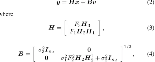
Fig. 2. Analytical and simulated p.d.f.s of the arbitrary eigenvalue of
U†tAUt, with system parameters: (3,2,3), P1 = P2 = 10dB, and
P3= 5dB.
where Γ(a, z) = z∞e−xxa−1dx is the complementary
in-complete gamma function.
Then, using the above result and (10), the ergodic capacity can be calculated as
C=
q
i=q−s+1
q
j=1 s
2 ln(2)C1(−1)
i+j|K i,j|
.
∞
0 ln(1 +ρλ)
λns−q+i−1
Γ(ns−q+i)Aλ(i, j)dλ
IB
(24)
where IB is given in (25). A closed form expression for
the integral, IC, in (25) is difficult to find but it can be
evaluated numerically. Again, note that when c1 > 0, the integral, IC, has a singular point at x =c2/c1. We use the
same approximation as in (20), and the region of integration is (0, c2/c1−/c1) to (c2/c1+/c1,∞).
By using the result in (24), the ergodic capacity of the system without the direct link can also be obtained as a special case. The derivation is omitted due to space limitation.
IV. RESULTS
The results produced in this paper are validated by using Monte Carlo simulation. In all results given, we have used the following conditions:
• The total transmitted power from the source is equal to
one, i.e.ρ= 1/ns,
Aλ(i, j) =
⎧ ⎪ ⎨ ⎪ ⎩
nd−j
t=0 e−
λ
c (nd−j)!
t!(nd−j−t)!(q−ns−nd+j)nd−j−tλ
tcq−ns−nd+j−1−t i= 1, . . . , q, j= 1, . . . , nd
∞
0 xj−nd−1 c4cx3+xc5
q−ns−1
e − λ
c3x c4x+c5
ξ(x)dx i= 1, . . . , q, j=nd+ 1, . . . , q
. (17)
Ki,j=
(i−nd+j)nd−jci−nd+j−1 i= 1, . . . , q, j= 1, . . . , nd
∞
0 xj−nd−1 c4cx3+xc5
i−1
ξ(x)dxIA(i, j) i= 1, . . . , q, j=nd+ 1, . . . , q ,
(19)
whereIA(i, j) =qv−=0i
q−i
v
c4 c1
v c
4c2
c1 +c5
q−i−vj+i+m−q−2 w=0
j+i+m−q−2 w
ci3−1e−c2/c1 cw1+1
c2 c1
j+i+m−q−2−w
IA1.
IA12= ⎧ ⎪ ⎨ ⎪ ⎩
−e−c1v+w−nd
k=0
(−1)v+w−nd−k(v+w−n d)!()k
k!(−1/c1)v+w−nd−k+1 v+w−nd≥0
(−1)nd−w−v(1/c
1)nd−w−v−1Ei(−/c1)
(nd−w−v−1)! +
e−/c1
()nd−w−v−1
nd−w−v−2
k=0 (−1)
k(1/c
1)k()k
(nd−w−v−1)(nd−w−v−2)...(nd−w−v−1−k) v+w−nd<0
.
(21)
IA11= ⎧ ⎪ ⎪ ⎪ ⎪ ⎪ ⎪ ⎨ ⎪ ⎪ ⎪ ⎪ ⎪ ⎪ ⎩
ec1v+w−nd
k=0 (−1)
v+w−nd−k(v+w−n d)!(−)k
k!(−1/c1)v+w−nd−k+1 −e c2
c1v+w−nd
k=0 (−1)
v+w−nd−k(v+w−n d)!(−c2)k
k!(−1/c1)v+w−nd−k+1 v+w−nd≥0
(−1)nd−w−v−1(1/c1)nd−w−v−1Ei(/c1)
(nd−w−v−1)! +
(−1)nd−w−v(1/c1)nd−w−v−1Ei(c2/c1)
(nd−w−v−1)!
− e/c1
(−)nd−w−v−1
nd−w−v−2
k=0
(−1)k(1/c1)k(−)k
(nd−w−v−1)(nd−w−v−2)...(nd−w−v−1−k)
+ ec2/c1
(−c2)nd−w−v−1
nd−w−v−2
k=0 (−1)
k(1/c
1)k(−c2)k
(nd−w−v−1)(nd−w−v−2)...(nd−w−v−1−k) v+w−nd<0
. (22)
IB=
⎧ ⎪ ⎨ ⎪ ⎩
nd−j
t=0 t!((nndd−−jj−)!t)!
(q−ns−nd+j)nd−j−t
Γ(ns−q+i) c
q−ns−nd+j−1−t
(1/ρ)ns+t−q+i(ns+t−q+i−1)!eρc1 ns+t−q+i
r=1 Γ(−(ns+t−q+i) +r,1/(ρc))(ρc)r i= 1, . . . , q, j= 1, . . . , nd
IC i= 1, . . . , q, j=nd+ 1, . . . , q
,
(25)
whereIC=
∞ 0 x
j−nd−1(n
s−q+i−1)!
Γ(ns−q+i) c4cx3+xc5
q−ns−1
(1/ρ)ns−q+iec4ρcx3+xc5 ns−q+i
k=1 Γ(−(ns−((qc+4xi+)+ck,5)(/c(4ρcx3+xc))5)k/(ρc3x))ξ(x)dx.
0 5 10 15 20 25 30
0 5 10 15
(2,2,2)
(2,2,3) (3,2,3)
P 1 (dB)
Mean Capacity (bit/s/Hz)
Theory
[image:4.612.49.572.56.571.2]Simulation
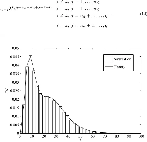
Fig. 3. Analytical and simulated ergodic capacity of the system with parameters:P1=P2= 1.5P3.
Furthermore, we set σ21 = σ22 = σ23 = 1, implying that the signal-to-noise ratios (SNR) of the links (S→D), (S→R) and (R→D) are P3, P1 and P2, respectively. In the results, the number of antennas used in the system is represented by the 3-tuple (ns, nr, nd). First, in Fig. 2, we validate the result
in Theorem 1 via simulation. The plots show the p.d.f. of
0 5 10 15 20 25 30
0 2 4 6 8 10 12 14 16 18 20
P3=0.1 P1 P
3=P1
P3=10 P1
P 1 (dB)
Mean Capacity (bit/s/Hz)
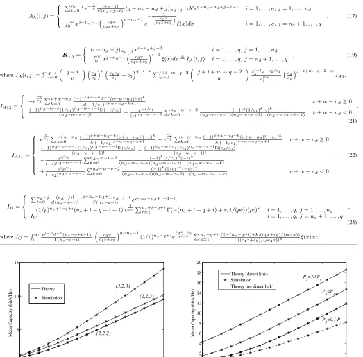
[image:4.612.57.295.416.596.2]Theory (direct link) Simulation Theory (no direct link)
Fig. 4. Analytical and simulated ergodic capacity of the system with parameters:(3,2,3)andP1=P2.
[image:4.612.323.552.418.600.2]the arbitrary eigenvalueλwith system configuration(3,2,3). Figure 2 shows that the analytical results are in agreement with the simulations.
10−1 100 101 2
3 4 5 6 7 8 9 10
P 3=20dB
P3 = 10dB
P 3 = 5dB
α
Mean Capacity (bit/s/Hz)
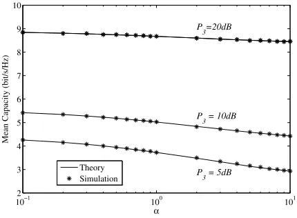
[image:5.612.67.282.55.213.2]Theory Simulation
Fig. 5. Analytical and simulated ergodic capacity of a(3,2,3)system vs.
α, whereP1=αP2= 10dB. Also shown is theS→Dlink power,P3.
configurations: (2,2,2),(2,2,3) and (3,2,3). The results are
given as a function of the SNR in the links as P1 = P2 =
[image:5.612.326.560.526.623.2]1.5P3. We see that the analytical results exactly match the simulations.
Figure 4 gives the performance of the analytical and simulated ergodic capacity of the system with configuration (3,2,3), when theS→Dlink strength varies. The results show that the capacity of the system improves with increases in the S→D signal strength due to diversity improvement. Note that whenP3=P1, the results in Appendix B are used to generate analytical results. We have also included the performance of the system without the direct link. Hence, Fig. 4 shows the performance gains of the system due to the inclusion of the direct link. Again the analytical results exactly match with the simulations.
Finally, Fig. 5 shows the performance of a (3,2,3) system
with varyingR→Dlink SNR. The SNR have the relationship
P1=αP2= 10dB. The results show that when P3 (the SNR
of the S→D link) is high there is not much improvement
in capacity even though P2 is increased. Also when P3 is
weak the capacity improvement due to increases inP2is more obvious.
V. CONCLUSIONS
The paper presents an ergodic capacity analysis of an AF MIMO two-hop system including the source to destination link. We first derived an expression for the probability density function of the unordered eigenvalue of the system and from that, a closed form expression for the ergodic capacity of the system is derived. We also validated the analysis by using simulations and both results match exactly. The results also show that having the direct link improves the capacity due to diversity and quantifies this improvement.
APPENDIX A. Proof of Theorem 1
The p.d.f. of λ, f(λ), can be calculated by using the result in (13). The eigenvalues of A, μ = {c, . . . , c, μ1, . . . , μl},
are related to the eigenvalues of H2H†2, ν = {ν1, . . . , νl}
via, μk = c4cν3kν+kc5. Then, using the result for f(λ|μ) in
(13), f(λ|ν) can be obtained by substituting μk = c4cν3kν+kc5
inf(λ|μ), as fixing the values ofμis equivalent to fixing the values ofν. Then usingf(λ|ν)andf(ν), the eigenvalue p.d.f f(λ) can be derived as shown below.
The matrix H2H†2 is Wishart or pseudo-Wishart [10]
depending on the dimension, nd×nr, of H2. However, the
non-zero eigenvalues of H2H†2 are the same irrespective of whether the matrix is Wishart or pseudo-Wishart. Hence the non-zero unordered eigenvalue p.d.f ofH2H†2 can be given as [13]
f(ν) = π
l(l−1)
l!CΓl(l)CΓl(m) l
k=1
νkm−le−νk
l
k<p
(νk−νp)2. (26)
Using the result in (13), the conditional p.d.f. f(λ|ν)can be obtained by substitutingμk= c4cν3kν+kc5 in (13) as
f(λ|ν) = 1
snd−1
k=1 k!(−1)q(q−1)/2(c3c5)l(l−1)/2
×l 1
k<p(νk−νp)
l
k=1
((cc4−c3)νk+cc5)nd (c4νk+c5)nd+l−1
×
q
k=q−s+1
λns−q+k−1
Γ(ns−q+k)|G|.
(27)
Then, using the relation f(λ,ν) = f(ν)f(λ|ν), f(λ,ν)
can be given as in (28). In (28), lk<p(νk − νp) =
(−1)l(l−1)/2|Φ
j(νi)|,Φi(νj) =νji−1,
C0= π
l(l−1)
l!CΓl(l)CΓl(m)
(−1)−ndl(−1)l(l−1)/2
snd−1
k=1 k!(−1)q(q−1)/2(c3c5)l(l−1)/2
,
(29)
ξ(νk) =νkm−le−νk
(c4νk+c5)q−1
(c1νk−cc5)nd, (30) andGis aq×qmatrix with entries given in (31).
Now f(λ) can be obtained by integrating over all νj by
using the method described inLemma 2of [14] as,
f(λ) =C0
q
k=q−s+1
λns−q+k−1
Γ(ns−q+k)
×
∞
0 . . .
∞
0
l
k=1
ξ(νk)|Φi(νj)| |G|dν1. . . dνl
C0l!
C1
q
k=q−s+1
λns−q+k−1
Γ(ns−q+k)
|Ψ| (32)
whereΨ is aq×qmatrix with entries given in (33).IA(i, j)
in (33) is given in (19). Finally, we obtain the result in Theorem 1 by using the Laplace expansion of (32).
B. Ergodic Capacity whenP1=P3
In this special case, when P1 =P3, the ergodic capacity of
the system can be obtained by using (24). However,Ki,j and
f(λ,ν) = π
l(l−1)
l!CΓl(l)CΓl(m)
(−1)−ndl
snd−1
k=1 k!(−1)q(q−1)/2(c3c5)l(l−1)/2
l
k=1
νkm−le−νk
(c4νk+c5)q−1
(c1νk−cc5)nd
l
k<p
(νk−νp) q
k=q−s+1
λns−q+k−1
Γ(ns−q+k)|G|
C0
q
k=q−s+1
λns−q+k−1 Γ(ns−q+k)
l
k=1
ξ(νk)|Φi(νj)| |G|. (28)
Gi,j=
⎧ ⎪ ⎪ ⎪ ⎪ ⎪ ⎪ ⎪ ⎪ ⎨ ⎪ ⎪ ⎪ ⎪ ⎪ ⎪ ⎪ ⎪ ⎩
(i−nd+j)nd−jci−nd+j−1 i=k, j= 1, . . . , nd
nd−j
t=0 e−
λ
c (nd−j)!
t!(nd−j−t)!(q−ns−nd+j)nd−j−tλ
tcq−ns−nd+j−1−t i=k, j= 1, . . . , nd
c3νj−nd
c4νj−nd+c5
i−1
i=k, j=nd+ 1, . . . , q
c3νj−nd
c4νj−nd+c5
q−ns−1
e−
λ(c4νj−nd+c5)
c3νj−nd i=k, j=n
d+ 1, . . . , q
. (31)
Ψi,j=
⎧ ⎪ ⎪ ⎪ ⎪ ⎪ ⎨ ⎪ ⎪ ⎪ ⎪ ⎪ ⎩
(i−nd+j)nd−jci−nd+j−1 i=k, j= 1, . . . , nd
nd−j
t=0 e−
λ
c (nd−j)!
t!(nd−j−t)!(q−ns−nd+j)nd−j−tλ
tcq−ns−nd+j−1−t i=k, j= 1, . . . , nd
xj−nd−1 c3x
c4x+c5
i−1
ξ(x)dxIA(i, j) i=k, j=nd+ 1, . . . , q
xj−nd−1 c3x
c4x+c5
q−ns−1
e−
λ(c4x+c5)
c3x ξ(x)dx i=k, j=nd+ 1, . . . , q
. (33)
Ki,j=
(i−nd+j)nd−jci−nd+j−1 i= 1, . . . , q, j= 1, . . . , nd
∞
0 xj−nd−1 c4cx3+xc5
i−1
ξ(x)dxIA(i, j) i= 1, . . . , q, j=nd+ 1, . . . , nd+l ,
(34)
whereIA(i, j) =ci3−1(−c2)−ndqv−=0i
q−i v
(c4)v(c5)q−i−vΓ(v+j+i+m−q−1).
IB=
⎧ ⎪ ⎨ ⎪ ⎩
nd−j
t=0 ( nd−j)!
t!(nd−j−t)!
(q−ns−nd+j)nd−j−t
Γ(ns−q+i) c
q−ns−nd+j−1−t(1/ρ)ns+t−q+i
(ns+t−q+i−1)!e 1
ρcns+t−q+i
r=1 Γ(−(ns+t−q+i) +r,1/(ρc))(ρc)r i= 1, . . . , q, j= 1, . . . , nd
IC i= 1, . . . , q, j=nd+ 1, . . . , q
, (35)
whereIC=2 cq3−ns−1
(−c2)nd
ns
v=0
ns
v
cv4c5ns−v0∞ln(1 +ρλ)λ
ns−q+i−1
Γ(ns−q+i)e
−λc4 c3 λc5
c3
v+j+m−ns−1 2
Kv+j+m−ns−1 2
!
λc5 c3
dλ.
Then, for this case, Ki,j andIB can be evaluated as given in
(34) and (35), respectively. Then, substituting (34) and (35) in
(24), the ergodic capacity of the system when P1 =P3 can
be obtained.
REFERENCES
[1] R. U. Nabar, H. B¨olcskei, and F. Kneubuhler, “Fading relay channels: Performance limits and space-time signal design,”IEEE J. Select. Areas Commun., vol. 22, no. 6, pp. 1099–1109, Aug. 2004.
[2] A. Sendonaris, E. Erkip, and B. Aazhang, “User cooperation diversity – part 1: System description,”IEEE Trans. Commun., vol. 51, no. 11, pp. 1927–1938, Nov. 2003.
[3] M. Herdin, “MIMO amplify-and-forward relaying in correlated MIMO channels,” inProc. Int. Conf. on Inform. Commun. and Signal Process-ing, Bangkok, Thailand, Dec. 6-9, 2005, pp. 796–800.
[4] X. Tang and Y. Hua, “Optimal design of non-regenerative MIMO wireless relays,”IEEE Trans. Wireless Commun., vol. 6, no. 4, pp. 1398– 1407, April 2007.
[5] H. B¨olcskei, R. U. Nabar, O. Oyman, and A. Paulraj, “Capacity scaling laws in MIMO relay networks,”IEEE Trans. Wireless Commun., vol. 5, no. 6, pp. 1433–1444, June 2006.
[6] J. Wagner, B. Rankov, and A. Wittneben, “On the asymptotic capacity of the Rayleigh fading amplify-and-forward MIMO relay channel,” in
Proc. IEEE Int. Symp. Information Theory (ISIT), Nice, France, June 24-29, 2007, pp. 2711–2715.
[7] V. Morgenshtern and H. B¨olcskei, “Crystallization in large wireless networks,” IEEE Trans. Inf. Theory, vol. 53, no. 10, pp. 3319–3349, Oct. 2007.
[8] A. Maaref and S. A¨ıssa, “Eigenvalue distributions of Wishart-type random matrices with application to the performance analysis of MIMO MRC systems,”IEEE Trans. Wireless Commun., vol. 6, no. 7, pp. 2678– 2689, July 2007.
[9] G. Alfano, A. Tulino, A. Lozano, and S. Verd´u, “Capacity of MIMO channels with one-sided correlation,” inProc. IEEE Int. Symp. on Spread Spectrum Techniques and Applications (ISSSTA), Sydney, Australia, Aug. 30-Sep. 2, 2004, pp. 515–519.
[10] R. K. Mallik, “The pseudo-Wishart distribution and its application to MIMO systems,”IEEE Trans. Inf. Theory, vol. 49, no. 10, pp. 2761– 2769, 2003.
[11] S. Jin, M. R. McKay, C. Zhong, and K.-K. Wong, “Ergodic capacity analysis of amplify-and-forward MIMO dual-hop systems,” in Proc. IEEE Int. Symp. Information Theory (ISIT), Toronto, Canada, July 6-11, 2008, pp. 1903–1907.
[12] M. Chiani, M. Z. Win, and H. Shin, “Capacity of MIMO systems in the presence of interference,” in Proc. IEEE Global Telecommunications Conf., San Francisco, California, USA, Nov. 30-Dec. 1, 2006, pp. 1–6. [13] T. Ratnarajah, R. Vaillancourt, and M. Alvo, “Complex random matrices and Rayleigh channel capacity,”Commun. Inf. Syst., vol. 3, pp. 119–138, 2003.