Quantitative analysis of the z spectrum using a numerically simulated look up table: application to the healthy human brain at 7T

Quantitative Analysis of the Z-Spectrum Using a

Numerically Simulated Look-up Table: Application

to the Healthy Human Brain at 7T

Nicolas Geades, Benjamin A. E. Hunt, Simon M. Shah, Andrew Peters,

Olivier E. Mougin, and Penny A. Gowland*

Purpose:To develop a method that fits a multipool model to z-spectra acquired from non–steady state sequences, taking into account the effects of variations in T1 or B1 amplitude and the results estimating the parameters for a four-pool mod-el to describe the z-spectrum from the healthy brain.

Methods: We compared measured spectra with a look-up table (LUT) of possible spectra and investigated the potential advantages of simultaneously considering spectra acquired at different saturation powers (coupled spectra) to provide sensi-tivity to a range of different physicochemical phenomena. Results: The LUT method provided reproducible results in healthy controls. The average values of the macromolecular pool sizes measured in white matter (WM) and gray matter (GM) of 10 healthy volunteers were 8.9%60.3% (intersubject standard deviation) and 4.4%60.4%, respectively, whereas the average nuclear Overhauser effect pool sizes in WM and GM were 5%60.1% and 3%60.1%, respectively, and aver-age amide proton transfer pool sizes in WM and GM were 0.21%60.03% and 0.20%60.02%, respectively.

Conclusions:The proposed method demonstrated increased robustness when compared with existing methods (such as Lorentzian fitting and asymmetry analysis) while yielding fully quantitative results. The method can be adjusted to measure other parameters relevant to the z-spectrum. Magn Reson Med 78:645–655, 2017. VC _{2016 The Authors Magnetic} Resonance in Medicine published by Wiley Periodicals, Inc. on behalf of International Society for Magnetic Resonance in Medicine. This is an open access article under the terms of the Creative Commons Attribution License, which permits use, distribution and reproduction in any medium, provided the original work is properly cited.

Key words:CEST; APT; NOE; MT; LUT; z-spectra

INTRODUCTION

Magnetization transfer (MT), chemical exchange satura-tion transfer (CEST), and nuclear Overhauser effect (NOE) phenomena use the transfer of magnetization, or exchange of protons or molecules, to sensitize the visible water proton pool to macromolecules or certain moieties (1). Conventional MT ratio images are sensitive to a com-bination of these effects depending on the frequency, power, and timing of the off-resonance saturation used. On the other hand, the z-spectrum (2) acquires MT ratio data at various frequency offsets, making it possible to investigate all of these phenomena.

However, quantifying the effects of these different pro-cesses in the z-spectrum remains a challenge, because radiofrequency (RF) irradiation used to probe the various pools will saturate more than one pool and will generally cause direct water saturation (DS). The spectrum is there-fore a mixture of MT, DS, NOE, and CEST signals, and the different components are difficult to separate (1,3–5). Early assessment of the CEST effect was based on asym-metry analysis (6), but this is confounded if independent changes occur on either side of the z-spectrum. More recent studies have used Lorentzian fitting (3,7) and Lor-entzian difference methods of analysis (8). These methods are relatively simple and may be adequate in some cir-cumstances (e.g., where the RF power is well controlled) but are not quantitative; this is because the effects of the different pools do not add linearly, particularly at high saturation powers, and because changes in T1 and RF power (9,10) will disrupt the results. Other methods attempt to suppress the MT contribution by applying dou-ble frequency irradiation (11,12), but the CEST effects are still diluted by MT and DS, even if isolated from them.

Steady state saturation is often used for MT imaging and quantification, with the drawback of high specific absorp-tion rate (SAR) and low signal-to-noise ratio (SNR) in the resulting images, but with the advantage of providing an analytical solution for z-spectra quantification. However, a pulsed saturation scheme that does not reach steady state provides increased SNR for high-resolution scanning with wide (three-dimensional [3D]) coverage. The drawback of the saturation not reaching a steady state is that it has prov-en difficult to analytically determine the signal in the z-spectra taking into account the effects of all possible field inhomogeneities. Meissner et al. (13) recently proposed an analytical method of simultaneously determining the con-centration and exchange rates of intermediate to fast exchanging protons in the case of pulsed presaturation. Thus far, a numerical computation of the evolution of the

Sir Peter Mansfield Imaging Centre, School of Physics and Astronomy, Uni-versity of Nottingham, Nottingham, United Kingdom.

Grant sponsor: Initial Training Network, HiMR, funded by the FP7 Marie Curie Actions of the European Commission; Grant number: FP7-PEOPLE-2012-ITN-316716; Grant sponsor: Medical Research Council; Grant spon-sor: MRC Doctoral Training Grant; Grant number: MR/K501086/1 (to B.A.E.H.); Grant sponsor: MRC UK MEG; Grant number: MR/K005464/1. *Correspondence to: Penny A. Gowland, PhD, Sir Peter Mansfield Imaging Centre, University Park, University of Nottingham, NG7 2RD, United King-dom. E-mail: [email protected]

Received 25 May 2016; revised 16 August 2016; accepted 16 August 2016 DOI 10.1002/mrm.26459

Published online 17 October 2016 in Wiley Online Library (wileyonlinelibrary. com).

VC _{2016 The Authors Magnetic Resonance in Medicine published by Wiley} Periodicals, Inc. on behalf of International Society for Magnetic Resonance in Medicine. This is an open access article under the terms of the Creative Commons Attribution License, which permits use, distribution and reproduction in any medium, provided the original work is properly cited.

Magnetic Resonance in Medicine 78:645–655 (2017)

various pools is considered the gold standard but involves a large computational cost (14). To avoid the computation-ally time-consuming requirement to simulate the z-spectra for every voxel, we propose a method of fitting z-spectra acquired in the pseudo–steady state by comparing the acquired spectra with a large predefined database of numer-ically simulated spectra based on the Bloch-McConnell equations. The database includes proton pool concentra-tions, B1 inhomogeneity, and T1 information.

One particular problem in quantifying z-spectra phe-nomena is sensitivity to RF saturation power. The z-spectrum is sensitive to different pools at different RF pow-ers depending on exchange rates, so inevitable variations in RF power setting and RF inhomogeneity will cause vary-ing sensitivity to different pools. We attempted to mitigate these problems by acquiring data at varying RF powers.

The aim of this study was to develop a new method of quantifying the separate proton pool concentrations from z-spectra of the human brain at 7T by using a look-up table (LUT) and taking T1 and B1 variations into account. The sensitivity of the approach was investigated using Monte Carlo simulations. It was tested for measuring MT, NOE, and amide proton transfer (APT) CEST in 10 healthy volunteers, and a repeatability study was also conducted.

METHODS

Model

Fundamentally, this method involved fitting the z-spectra to a model based on the Bloch-McConnell equa-tions. However, given the computational time required to simulate model spectra in a non–steady state, mea-sured spectra were instead compared with a LUT (data-base of simulated spectra) calculated in advance, similar to the dictionaries used in MR fingerprinting (15).

A four-pool version of the modified Bloch-McConnell equations was used to create a database of simulated z-spectra. The model assumes four interacting pools of protons that consist of 1) the free water magnetization (free pool, M0f), 2) macromolecules and the hydration

layer (bound pool, Mb

0), 3) small proteins in chemical

exchange with the free pool at a single frequency, in this case considering APT (exchanging pool,Mc

0), and 4)

pro-tons experiencing dipole cross-relaxation through space with the free water magnetization (NOE pool,Mn

0). The

Bloch-McConnell equation can be summarized as (16)

dMðt;vrfÞ

dt ¼Aðt;vrfÞMðt;vrfÞ þBM0: [1]

whereMis a vector describing the time evolution of each of the proton pools, andAandBare matrices describing the effect of RF saturation, exchange between each proton pool and the free water pool, longitudinal relaxation rates of each proton pool, and the line shape of the bound pool. A full description of this model and its numerical implementation is given elsewhere (17). It is assumed that each pool can be described by a single transverse relaxation time T2, except for the macromolecular associated pool, which is assumed to be described by a super-Lorentzian line shape (18–21) centered at2.4 ppm relative to water. It is also assumed

that all pools are in exchange with the water pool but that direct exchange between the other pools is negligible.

No simple analytical solution to this equation exists in the approach to steady state, so instead an ordinary dif-ferential equation solver was implemented to compute the evolution of the magnetization of the different pools during the approach to saturation, using a 4th-order Runge-Kutta algorithm with a 5-ms interval, taking into account the satu-ration and readout pulses used to reach the center of k-space. This yielded the longitudinal magnetization in the free water pool (Mzf) in the simulated z-spectra.

Estimating Parameters from an LUT

Z-spectra were simulated for the RF saturation train used to acquire in vivo spectra (20 Gaussian-windowed sinc RF pulses of bandwidth¼200 Hz, 30 ms long, repeated every T¼60 ms, for a 50% duty cycle), at 15 different off-resonance frequencies of the saturation pulse (Table 1). The choice of off-resonance frequencies was deter-mined by examining the full width at half maximum of fitted Lorentzian curves. The different pools were sam-pled at frequencies corresponding to their maximum amplitude and full width at half maximum, with more frequencies and therefore more weighting given to the NOE and MT pools. A 50-kHz off-resonance saturation was also simulated for normalization of the spectrum.

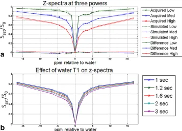
Because different saturation pulse powers provided sensi-tivity to the different pools (Fig. 1a), we investigated the potential advantages of simultaneously fitting coupled spec-tra acquired at powers of one, two, or three to optimize the fitting across the different pools. Spectra were simulated for nominal B1sat (maximum RF amplitudes as defined in

Fig. 2) of 1.9mT, 3.8mT, and 6.34mT at 50% duty cycle (equivalent to 0.38mT, 0.75mT, and 1.25mTB1rms). Spectra

were simulated for a range of pool concentrations and T1 values (Fig. 1b) of the free water pool, assuming the other physical parameters shown in Table 1. The T1 of the free pool was estimated from the observed T1 and the T1 of the other proton pools, as described previously (17,22). Given the variability in the literature, the exchange rates used in this simulation were selected experimentally by initially performing a full fit to spectra from ROIs.

Unfortunately, it is impossible to control the B1 ampli-tude throughout the volume of interest, particularly at ultrahigh fields, and this inhomogeneity will alter both

B1satandB1read(Fig. 2). Therefore, three coupled spectra

were simulated (i.e., with different values of B1sat but

the same values of B1read) for various B1 scaling factors

to account for the effect of B1 inhomogeneity or RF mis-adjustment. Linear interpolation was used to extend the simulated database (Table 1; simulated for three B1sat values; six B1scale values; eight MT, NOE, and APT val-ues; and five T1 values [46,080 spectra]) to yield spectra for three values ofB1sat; 16 B1 scaling factors; 17 T1

The proton pool fractions were then estimated by com-paring the experimentally measured spectra to the LUT by brute force least-squares fitting. This involved calcu-lating the sum-of-squares difference between the acquired spectrum and every spectrum in the LUT sepa-rately, and then selecting the parameters of the

simulated spectrum with the smallest residual. This restricted possible fitted values only to the simulated or interpolated values. When fitting coupled triplets (or pairs) of spectra acquired at the three aforementioned values ofB1sat, the sum-of-squares difference was found

between the three measured spectra (acquired with fixed

FIG. 1. (a) Experimentally mea-sured single WM voxel (solid) spectra compared with the fitted (dotted) spectra acquired at

B1rms¼0.38 (green), 0.75 (blue), and 1.25mT (red). The difference between the acquired and simu-lated spectra (acquired simu-lated) is also shown. These three spectra were fitted as a coupled set of spectra acquired at three predefined powers, but they could also be fitted individually. (b) Effects of water T1 on simu-lated z-spectra.

Table 1

Physical Parameters Used in the Simulation of the Database (LUT)

Relative Concentration

(M0%) T1 (s)

T2 (ms)

Exchange Rate with

Free Water Pool (Hz)

Chemical Shift (ppm)

Off-Resonance Saturation Frequencies

(in ppm)

B1

Amplitude B1 Scaling

Free water

pool (DS) –

Five values (1, 1.2, 1.6, 2,

and 3 s)

40 – 0

16.7

6.7

4.7

4

3.5

3

2.3

1 0 1 2.5 3.5 4.5 6.7 16.7

Nominal B1 amplitudes of

0.38, 0.75, and 1.25mT

B1rms

Saturation and imaging pulses scaled by 30%, 60%, 80%, 100%, 120%,

and 150% Bound

pool (MT)

Eight values (0.1%, 1%, 2%, 5%, 8%,

10%, 12%, and 15%)

1 0.009 50 2.4

NOE pool

Eight values (0.1%, 1%, 2%, 3.5%, 5%, 6%, 8%,

and 10%)

1 0.3 10 3.5

CEST pool (APT)

Eight values (0.02%,

0.05%, 0.075%, 0.1%, 0.2%, 0.3%, 0.5%, and 1%)

ratios of B1sat) and sets of spectra simulated with the

same known ratios ofB1sat. The results of this fitting are

shown in Fig. 1a.

Monte Carlo Simulations

Monte Carlo simulations were used to investigate the robustness of the fit, focusing particularly on the effect of variations in B1 amplitude. Realistic levels of uni-formly distributed noise (therand function in MATLAB [MathWorks, Natick, Massachusetts, USA]) was added to a simulated spectrum, which was then fitted to the LUT. This was repeated for 10,000 realizations of the noise to determine the resulting variance in the fitted parameters. The spectra were simulated forMb

0¼10%,M0n¼6%, and Mc

0¼0.25%, T1¼1.2 s and the 3 nominal B1sat

ampli-tudes shown in Table 1 (initially with scaling factor of 100%). 2% noise relative to the normalized M0 was added to each spectral point (assuming 8 min to acquire full spectrum), 10% noise was added to the T1 map acquired in a 10-min scan and 5% noise was added to the B1 map acquired in a 3-min scan.

Because we know that the results of z-spectrum fitting are very sensitive to saturation power, we compared the effect of data acquired at one, two, or three coupled pow-ers. We adjusted the noise in the simulated z-spectra to compensate for the necessary changes in the scan time at each power if the total scan time were to be kept con-stant (i.e., one spectrum at a single power with 1.15%

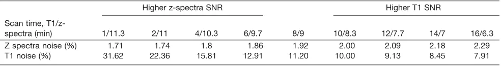
noise or three spectra at three powers with 2% noise each) (Fig. 3). For a given total acquisition time, the times allowed to acquire the z-spectra and T1 map were also counter-varied as shown in Table 2 (i.e., as the time given to z-spectrum imaging was reduced, the time given to T1 mapping increased, with the corresponding image noise levels being adjusted to maintain an SNR/time in each scan and constant total acquisition time). For a total acqui-sition time of 34 min, the times allowed to acquire the T1 map and z-spectra at three powers were varied from 1 to 16 min and 11 to 6 min per power, respectively, so that the noise in the T1 map varied from 31% to 8% and the noise in the z-spectra varied from 1.7% to 2.2%.

Finally, the simulations were used to conduct a sensi-tivity analysis exploring the effects of B1 and T1 errors on MT, NOE, and APT.

Data Acquisition

Approval for human scanning was obtained from the University of Nottingham Medical School Ethics Com-mittee. Ten healthy subjects (women, n¼6; men, n¼4; age range, 19–62 y) were scanned at 7T (Philips, Best, Netherlands, Achieva, using a 32-channel Nova head receive array) with a protocol based on the results of the Monte Carlo simulations (three z-spectra scanned at dif-ferent powers with approximately 2% noise, T1 map with approximately 10% noise, and B1 map and B0 maps) to assess intersubject variation. Another three sub-jects (men, n¼2, ages 29 and 34 y; women, n¼1, age 52 y) were scanned three times, each with exactly the same protocol to assess intrasubject repeatability.

Each point on the z-spectrum was acquired using a saturation-prepared 3D turbo field echo (TFE) sequence (17) (Fig. 2). The saturation consisted of a train of 20 Gaussian-windowed sinc RF pulses of bandwidth¼

200 Hz and duration¼30 ms that were repeated every 60 ms (50% duty cycle), with a phase increment between each pulse and a spoiler gradient applied at the end of the train to remove any residual transverse magnetiza-tion. Z-spectra were acquired by varying the off-resonance saturation frequency as shown in Table 1, including a scan at 50 kHz off-resonance for normaliza-tion. (Normalization with no saturation produced an

FIG. 3. Mean and standard deviation in MT, NOE, and APT fit for different power combinations. The noise level assumed for each point in the z-spectrum was 1.15% for the single power (equivalent to 25 min/scan), 1.41% for two powers (equivalent to 12.5 min/scan), and 2% for three powers (equivalent to 8 min/scan). T1 noise was 10% and B1 noise was 5%. Relative SNR was calculated relative to the SNR of an 8-min scan.

offset on the spectra, consistent with RF amplifier droop during the readout pulses). This was repeated for the three nominal values ofB1satgiven in Table 1. The

imag-ing readout was a volume acquisition with a readout train of 410 gradient echoes, echo time¼2.7 ms, pulse repeti-tion time¼5.8 ms, flip angle¼8_{, field of view}

(FOV)¼19219260 mm3, 1.5 mm isotropic image reso-lution, low-high k-space acquisition, and a SENSE factor Right-Left (RL) of 2. The 3D volume acquisition required five repetitions of this cycle. Using this 3D non–steady state approach, a 15-point z-spectrum (plus an additional point for normalization), was acquired in 8 min (24 min total for the three powers). The amplitude of readout pulses was modulated to avoid large variations in signal at the start of the TFE train; there were two (np) ramped RF pulses before acquisition, followed by four (na) ramped RF pulses at the start of the acquisition, with the remaining pulses at constant flip angle of 8 _(B1

read, Fig. 2). In

addition, a B0 map (double echo method, FOV¼252

255100 mm3 _{at 332 mm}3 _{voxels) was acquired for} B0 correction (1 min), along with a whole head B1 map (dual TR method, at 20 ms and 120 ms TR, FOV 205180132 mm3at 3.244 mm3voxels, 3 min) and a T1 map (dual readout Phase-Sensitive Inversion Recovery (PSIR) data, FOV¼240216160 mm3at 0.8 mm isotro-pic resolution, SENSE factor [RL] of 2.2 and Foot-Head [FH] of 2, 10 min) yielding a total scan time of 38 min.

Data Preprocessing

Each z-spectra dataset was motion-corrected using FSL’s (23)mcflirt function, and then all were registered to the same space using a high contrast-to-noise ratio (CNR) image created by averaging across the dynamics of the z-spectrum acquired at the highest B1sat. SPM8 (24) was used to segment white matter (WM) and gray matter (GM) masks from the PSIR images that were retrospec-tively registered onto the high CNR image. The masks were thresholded at high probability values (0.9) to avoid partial volume errors. Similarly, the B0, B1, and T1 maps were registered onto the high CNR image space. B0 correction of all the z-spectra datasets was performed voxel-wise prior to the fitting by shifting the whole spec-trum based on the difference between the zero point (DS) and B0 map as described previously (4,6). Regions with very high B0 shift (>200 Hz) were removed from subsequent analysis because the spectra were too differ-ent from the simulated spectra.

Fitting the Experimental Data

The coupled spectra acquired at three different nominal values ofB1sat(and constant values ofB1read) were fitted

simultaneously to the database by calculating the total

sum of squared error between the three measured spectra and a set of three spectra simulated for the same ratio of actual saturation powers and same actual readout pulse amplitudes. The B1 map provided a B1 scaling factor linking the nominal and actual RF powers (and hence

B1sat andB1read) in each voxel. We also recorded the RF

drive scales from the Philips scanner for the B1 map and z-spectra acquisitions to allow the B1 map to be scaled to match the drive scales if necessary. The mean and standard deviation RF drive scale in the 10 z-spectra and B1 scans were 0.3460.03 and 0.3560.06, respectively. However, data collected with an RF drive scale of<0.22 (a fault state) were discarded since they produced spec-tra with B1sat so low that it lay outside the simulated

range. The T1 map also constrained the search. The fitting was done pixel-wise to create maps ofMb

0,M0n

andMc

0. Average values ofM0b,M0n, andM0cwere estimated

by averaging the fitted values over the WM and GM masks for the intersubject variation study, and over ROIs of about 500 voxels in three regions of the corpus callosum for intra-subject repeatability. As a test of the fitting procedure, we also investigated the possibility of fitting the three spectra for B1 scaling factor as well as pool sizes because the varia-tion in the z-spectra with RF amplitude is so large.

Finally, for comparison the spectra were also fitted using the qualitative Lorentzian fitting (25) method. Four Lorentzian curves (water, MT, NOE, and APT) were fitted using least-squares curve fitting and, to remove the effect of B1 inhomogeneity in the Lorentzian maps and hence allow a fair comparison with the LUT approach, we inter-polated the results from the three different powers to those expected forB1rms¼0.5mT. The pools were quantified as

the area under the curve for each fitted curve. We also per-formed standard asymmetry analysis for comparison (26).

RESULTS

Monte Carlo Simulations

Figure 3 shows the mean and standard deviation in the fitted values when the z-spectra were simulated and fit-ted at only a single target power (low [L], medium [M], or high [H]) at two target powers (LþM, MþH, or LþH) or at three target powers (LþMþH). The resulting mean fitted values were all within 1% of the original simulat-ed values. The different combinations of power benefit-ted from different measures. For instance, fitting the APT signal benefitted from all the acquisitions being made at lower powers, whereas this increased the noise in the fit for the MT pool. The results show that if RF power is well controlled, then medium power yields a reasonable fit across all three pools considered here (APT, NOE, and MT). In reality, especially at 7T, B1 is not well controlled and scanning at only one power

Table 2

Scan Times for T1 Scan and Single Power z-Spectra Scan with Corresponding Simulated T1 and z-Spectra Scan Noise

Higher z-spectra SNR Higher T1 SNR

Scan time,

T1/z-spectra (min) 1/11.3 2/11 4/10.3 6/9.7 8/9 10/8.3 12/7.7 14/7 16/6.3

Z spectra noise (%) 1.71 1.74 1.8 1.86 1.92 2.00 2.09 2.18 2.29

increases the risk of losing data in outlying regions of B1 amplitude. For this reason, we chose to scan and fit for three powers.

Figure 4a shows how the random error in the fitted val-ues changed as the partition of the acquisition time between the T1 map and z-spectra was counter-varied while keeping the total acquisition time constant. The lowest random error in the fitted MT and NOE values was achieved when T1 map noise was 10% and z-spectra noise was 2%, corresponding to acquisition times of 10 min and 8 min, respectively. On the other hand, the lower APT sig-nal benefitted from a longer z-spectra scan.

Figure 4b shows the systematic errors in estimated val-ues of MT, NOE, and APT caused by errors in the assumed values of B1 and T1. A 5% error in B1 resulted in a 10% error in MT, a 5% error in NOE, and a 10% error in APT, whereas a 10% error in T1 resulted in errors in MT, NOE, and APT of <5%. This highlights the requirement for accurate B1 knowledge when fitting z-spectra.

Experimental Results

The fit took 10.5 min for 274,000 voxels typically con-tained in a mask on a dual-core 3.3 GHz Intel Core

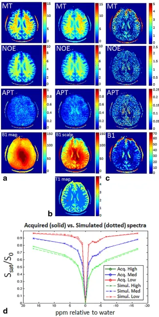
i3-3220 processor. Figure 5a shows MT, NOE, and APT maps produced by fitting data acquired on a healthy vol-unteer and the B1 map used in the fit, and Fig. 5d shows the fitted spectra from a single WM voxel. Figure 5 also compares the results of the fitting when including prior information from a separately acquired B1 map (Fig. 5a) or fitting the z-spectra for MT, NOE, APT, and the B1 scaling factor together (Fig. 5b). The difference between the two is shown in Fig. 5c. There is reasonable agree-ment between the MT, NOE, and APT maps produced by both fits and between the fitted and separately measured B1 map, although there is some mixing of information between the fitted value of B1 scale and MT as can be seen in the gray matter sulci.

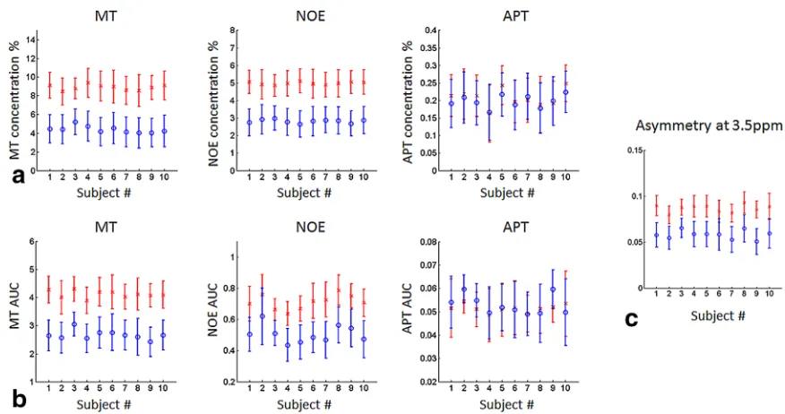
Figure 6a shows the average GM and WM pool sizes for 10 healthy subjects fitted using the LUT approach assuming prior information from B1 and T1 maps. Figure 6b shows the results of the same data analyzed using B1-corrected Lorentzian fitting (25). Figure 6c shows asym-metry analysis computed at 3.5 ppm. The standardized difference (27) between WM and GM was calculated for each pool, together with coefficient of variation. Table 3 summarizes the quantitative results.

FIG. 4. (a) Percentage error in MT (assuming Mb

0¼10%), NOE

(Mn

0¼6%) and APT (Mc0¼0.25%)

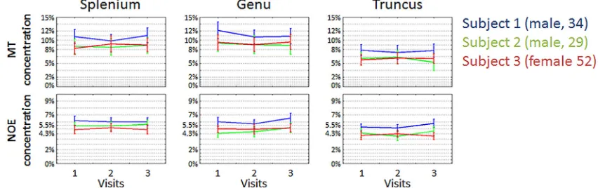
The intrasubject reproducibility results are also shown in Table 3 and in Fig. 7, with the error bars indicating the standard deviation across the voxels within the ROIs.

DISCUSSION

This study presents a novel method of deriving quanti-tative CEST information from any pulse sequence using a numerically derived database of possible z-spectra tai-lored to the acquisition protocol, and taking into account variations in RF amplitude and T1. A Monte Carlo simulation was used to investigate the sensitivity of the results to different acquisition protocols and errors in the estimates of B1 and T1. The procedure was used to estimate z-spectrum parameters using data acquired from 10 healthy subjects, with intrasubject reproducibility being assessed in a further three sub-jects. The results suggest that this method could be

used for reliable detection of the MT and NOE pools in the WM and GM of a healthy brain. Figure 6 shows the results of the intersubject repeatability study (mean and standard deviation over the whole WM or GM: standard error would be two orders of magnitude smaller) and demonstrates that the estimated parameters are reasonably consistent between subjects. The results from asymmetry analysis at 7T are difficult to interpret, because multiple effects contributed to the resulting metric. For this reason, asymmetry analysis is unsuit-able at high fields (>3T), and the results presented here show that asymmetry analysis is less sensitive than more quantitative metrics. The reproducibility study (Fig. 7; averaging over small ROIs in the corpus cal-losum) indicates that intersubject variation is dominat-ed by differences between individuals rather than measurement noise. These data will provide normative information for future studies.

FIG. 6. (a) Mean and standard deviation of MT, NOE, and APT values from WM (red) and GM (blue) masks for 10 healthy subjects. (b) B1-corrected Lorentzian-fitted mean and standard deviation of MT, NOE, and APT from the same WM and GM masks. In Lorentzian fit-ting, the pools are quantified as the area under the curve for each fitted curve. (c) Asymmetry at 3.5 ppm.

Table 3

Comparison of Quantitative Results for the Intersubject and Intrasubject Studies

Mb

0 Mn0 Mc0

Intersubject variability in 10 subjects (mean and standard deviation in mean across subjects) (Fig. 6)

LUT pool size for WM 8.9%60.3% 5.0%60.1% 0.21%60.03% LUT pool size for GM 4.4%60.4% 3.0%60.1% 0.20%60.02% Standardized difference

GM/WM, LUT fitting

7.8 7 0.07

Standardized difference GM/WM, Lorentzian fit

3.8 0.9 0.03

Standardized difference GM/WM, Asymmetry measure at 3.5ppm

0.43

Intrasubject repeatability in three

subjects (Fig. 7)

Average standard deviation in pool size (pool size in %), averaged over voxels

and subjects (from LUT method)

As reported elsewhere, the APT pool was found to be very small in the healthy brain but elevated in various pathologies, and it was too small to be detected reliably in the GM of these healthy subjects. However, the sequence used here could be better optimized for APT— for instance, by acquiring data only at lower power and by better sampling the APT z-spectrum peak. In this study, we assumed an APT exchange rate from previous in vivo measurements (28) and our own full fit to Bloch-McConnell equations, although lower values are often assumed (29). Using a lower value in the simulations would have increased the measured pool size. The APT peak is also very close to the amine peak at 1.8 ppm, which is thought to be in fast exchange [>1000 s1(29)] and, like many studies of APT, it is possible that these APT measures will have been contaminated by amines.

The LUT approach has various advantages over cur-rent quantification methods. Our approach is fully quan-titative, simple, time efficient, and allows simultaneous fitting of multiple parameters and overlapping peaks (even NOE and APT overlap due to the short T2 of the NOE). However, the method has some limitations. The LUT is initially computationally intensive to calculate, although it can be expanded post hoc to incorporate oth-er sequences. The fitted values are restricted to the exact simulated ones, but further precision can be achieved by simulation of more values or interpolation between values. A further refinement would be to use more ad-vanced interpolation methods based on the physical rela-tionship between CEST effects and RF amplitude (30). Similarly, in this study regions with B0 shift above 200 Hz were not analyzed, because such spectra had not been included in the data base; alternatively, the B0 shift could be included in the simulated database.

The LUT currently assumes constant exchange rate parameters, which can have an effect on the z-spectrum similar to that for pool concentration and which are sensi-tive to pH, which can change in pathology. The effects of exchange rate and concentration could be separated by increasing the dimensions of the LUT to include more acquisition parameters, including pulse duration and duty cycle. Similarly, it could be extended to include more pools and different relaxation times for each pool. These extensions would likely require the data acquisition to be tuned to give sensitivity to the parameters of interest.

WM and GM masks were aggressively thresholded to avoid partial volume errors, and the MT and NOE results showed very good WM/GM separation (Fig. 6a) and also variation across WM (Fig. 7). It is interesting to note that the NOE and MT values appear to be uncoupled in the corpus callosum, with the MT/NOE ratio varying bet-ween the truncus and the splenium and genu. Previous investigators have suggested that the truncus and genus have more myelinated axons than the splenium (31), so this may indicate a difference in sensitivity of the NOE and MT signals to myelination; alternatively, this result may relate to the previously reported dependence of MT on fiber orientation (20). In practice, a small positive APT pool was measured in all GM and WM ROIs. How-ever, given that the fit is based on a database of realistic spectra, no negative results are possible, which will bias the results at low signal (the noise distribution it is like-ly to be Rician).

Previously reported macromolecular pool concentra-tions for healthy WM range from 10% (32,33) to 15% (34) or higher (35), but assume different models and different physical parameters for the different pools. Two pool models (34–36) tend to overestimate the macromolecular pool concentration by effectively including the NOE pool. A previous study (28) that used a four-pool model (free water, MT, NOE, and APT) found somewhat lower MT and NOE pool concentrations of 6.2% and 2.4% in WM, assuming different values of T1b, T2, and exchange rates for the MT and NOE pools and a Lorentzian line shape for the bound pool. The same study measured an APT WM pool size of 0.22%, which is comparable to that measured here. The results depend on how physically realistic the model is. A recent study (37) suggested that aromatic NOE signals underlie the APT peak. Further work is required to determine whether this can be separated from APT—for instance, by making assumptions about the fraction of the NOE signals (37).

The sensitivity of the new LUT method is highlighted by the standardized difference between GM and WM for all pool size estimates (Table 3) which were considerably larger than for the semiquantitative Lorentzian fitting, even taking account of B1 variations in Lorentzian fitting method. The intrasubject variability (Fig. 7, measured in

500 voxels) was somewhat higher than that predicted from the Monte Carlo results (Fig. 3). There are several

potential reasons for these differences. First, the T1 values included in the simulations for the LUT were not long enough to model cerebrospinal fluid. Second, flow may have modified the effect of the saturation. Third, any errors in other fitted parameters may have led to changes in B1 being interpreted as change in MT due to the simi-larity of their effects on the spectra. There is some evi-dence for this in Fig. 5, where the difference between the maps calculated by fitting B1 and using a B1 map is partic-ularly obvious in regions of low B1 in the frontal lobes. This problem could be addressed by extending the LUT to lower powers. In terms of random errors, the B1 scaling factor was generally less than 100% (i.e., the LUT con-tained spectra simulated at higher power than that achieved experimentally). Furthermore, the fit assumed that the B1 scaling factor was constant across all scans on a particular subject, but we could use the scanner RF drive scale to correct for unexpected changes in RF output. We also showed that the most robust results were achieved by acquiring a separate T1 map rather than fitting the z-spectra for T1 (Fig. 4).

The simulations indicate that acquiring data at three coupled RF powers can result in a fit that is robust across different pools, whereas if sensitivity to only one particular pool is required, then fewer powers should be used. However, this assumes that the RF power is completely predictable and known before the experi-ment, whereas in practice, inhomogeneities in the RF field or variations in the adjustment of the RF amplitude are likely at 7T. Combined with the strong dependence of the results on RF power (confirmed in Fig. 4b), this suggests that acquiring spectra at a range of powers will reduce the risk of not being at the optimum power for any given pool. The method is sufficiently robust for the B1 scaling factor to be fitted directly from the z-spectra without acquiring a B1 map (Fig. 5b). Monte Carlo simu-lations suggest that this might be an optimal approach (data not shown), but in practice it was found to be unstable (e.g., GM contrast in the fitted B1 scaling map). This result suggests that the T2 or exchange rates assumed for the MT pool may not be correct in all loca-tions. The LUT approach can be extended to measure these parameters, provided the sequence is adapted to provide sensitivity to them [e.g., by varying the inter-pulse interval in the saturation (29,30)].

CONCLUSION

Quantifying proton pool concentrations from z-spectrum data has proved to be challenging. Data from steady state sequences can be fitted to analytical expressions but non–steady state sequences have advantages in terms of sensitivity (38), specific absorption rate, and flexibility in the saturation to provide sensitivity to the T2 of the bound pool and exchange rate. Methods that model the spectra as a sum of Lorentzian lines neglect the nonline-ar effect of overlapping contributions to the z-spectrum, and it is too computationally expensive to fit the full numerical model to the spectra. This study presents a new method of fitting data from non–steady state sequences in a feasible computational time by comparing z-spectra to a LUT using a priori knowledge of B1

scaling and T1. This method yielded reproducible results in healthy controls, with WM values forMb

0,M0n, andM0c

varying between 7% and 11%, 4% and 6%, and 0.1% and 0.3%, respectively, and GM values ranging between 3% and 6.5%, 1.8% and 3.5%, and 0.1% and 0.3%, respectively. The LUT is being extended to include the range of parameters expected in pathology or in other tis-sue. It could also be extended to fit for the T2s or exchange rates if experiments were designed to provide sensitivity to these parameters.

REFERENCES

1. van Zijl PCM, Yadav NN. Chemical exchange saturation transfer (CEST): what is in a name and what isn’t? Magn Reson Med 2011;65: 927–948.

2. Bryant RG. The dynamics of water-protein interactions. Annu Rev Biophys Biomol Struct. 1996;25:29–52.

3. Zaiss M, Schmitt B, Bachert P. Quantitative separation of CEST effect from magnetization transfer and spillover effects by Lorentzian-line-fit analysis of z-spectra. J Magn Reson 2011;211:149–155.

4. Zaiss M, Bachert P. Chemical exchange saturation transfer (CEST) and MR Z-spectroscopy in vivo: a review of theoretical approaches and methods. Phys Med Biol 2013;58:R221–R269.

5. Zaiss M, Xu J, Goerke S, Khan IS, Singer RJ, Gore JC, Gochberg DF, Bachert P. Inverse Z-spectrum analysis for spillover-, MT-, and T1-corrected steady-state pulsed CEST-MRI – application to pH-weighted MRI of acute stroke. NMR Biomed 2014;27:240–252. 6. Zhou J, Payen J-F, Wilson DA, Traystman RJ, van Zijl PCM. Using the

amide proton signals of intracellular proteins and peptides to detect pH effects in MRI. Nat Med 2003;9:1085–1090.

7. Jones CK, Polders D, Hua J, Zhu H, Hoogduin HJ, Zhou J, Luijten P, Van Zijl PCM. In vivo three-dimensional whole-brain pulsed steady-state chemical exchange saturation transfer at 7 T. Magn Reson Med 2012;67:1579–1589.

8. Dula AN, Arlinghaus LR, Dortch RD, Dewey BE, Whisenant JG, Ayers GD, Yankeelov TE, Smith SA. Amide proton transfer imaging of the breast at 3 T: establishing reproducibility and possible feasibility assessing chemotherapy response. Magn Reson Med 2013;70:216–224. 9. Desmond KL, Stanisz GJ. Understanding quantitative pulsed CEST in

the presence of MT. Magn Reson Med 2012;67:979–990.

10. Sun PZ, Sorensen AG. Imaging pH using the chemical exchange satu-ration transfer (CEST) MRI: correction of concomitant RF irradiation effects to quantify cest MRI for chemical exchange rate and pH. Magn Reson Med 2008;60:390–397.

11. Scheidegger R, Vinogradov E, Alsop DC. Amide proton transfer imag-ing with improved robustness to magnetic field inhomogeneity and magnetization transfer asymmetry using saturation with frequency alternating RF irradiation. Magn Reson Med 2011;66:1275–1285. 12. Lee JS, Regatte RR, Jerschow A. Isolating chemical exchange

satura-tion transfer contrast from magnetizasatura-tion transfer asymmetry under two-frequency rf irradiation. J Magn Reson 2011;215:56–63.

13. Meissner J-E, Goerke S, Rerich E, Klika KD, Radbruch A, Ladd ME, Bachert P, Zaiss M. Quantitative pulsed CEST-MRI using V-plots. NMR Biomed 2015;28:1196–1208.

14. Chappell MA, Donahue MJ, Tee YK, Khrapitchev AA, Sibson NR, Jezzard P, Payne SJ. Quantitative Bayesian model-based analysis of amide proton transfer MRI. Magn Reson Med 2013;70:556–567. 15. Ma D, Gulani V, Seiberlich N, Liu K, Sunshine JL, Duerk JL,

Griswold MA. Magnetic resonance fingerprinting. Nature 2013;495: 187–192.

16. Woessner DE, Zhang S, Merritt ME, Sherry AD. Numerical solution of the Bloch equations provides insights into the optimum design of PARACEST agents for MRI. Magn Reson Med 2005;53:790–799. 17. Mougin O, Clemence M, Peters A, Pitiot A, Gowland P.

High-resolu-tion imaging of magnetisaHigh-resolu-tion transfer and nuclear Overhauser effect in the human visual cortex at 7 T. NMR Biomed 2013;26:1508–1517. 18. Morrison C, Henkelman RM. A model for magnetization transfer in

tissues. Magn Reson Med 1995;33:475–482.

20. Pampel A, Muller DK, Anwander A, Marschner H, M€ oller HE. Orien-€ tation dependence of magnetization transfer parameters in human white matter. Neuroimage 2015;114:136–146.

21. Wilhelm MJ, Ong HH, Wehrli FW. Super-Lorentzian Framework for Investigation of T2* Distribution in Myelin. In Proceedings of the 20th Annual Meeting of ISMRM, Melbourne, Victoria, Australia, 2012. p. 2394.

22. Ramani A, Dalton C, Miller DH, Tofts PS, Barker GJ. Precise estimate of fundamental in-vivo MT parameters in human brain in clinically feasible times. Magn Reson Imaging 2002;20:721–731.

23. Jenkinson M, Beckmann CF, Behrens TEJ, Woolrich MW, Smith SM. FSL. Neuroimage 2012;62:782–790.

24. Penny DW, Friston JK, Ashburner TJ, Kiebel JS, Nichols ET, editors. Statistical parametric mapping: the analysis of functional brain images. London, UK: Academic Press; 2007. 656 p.

25. Windschuh J, Zaiss M, Meissner JE, Paech D, Radbruch A, Ladd ME, Bachert P. Correction of B1-inhomogeneities for relaxation-compensated CEST imaging at 7T. NMR Biomed 2015;28:529–537. 26. Guivel-Scharen V, Sinnwell T, Wolff SD, Balaban RS. Detection of

proton chemical exchange between metabolites and water in biologi-cal tissues. J Magn Reson 1998;133:36–45.

27. Yang D, Dalton J. A Unified Approach to Measuring the Effect Size Between Two Groups Using SAS. In Proceedings of the SAS Global Forum, Orlando, Florida, 2012. Paper 335.

28. Liu D, Zhou J, Xue R, Zuo Z, An J, Wang DJJ. Quantitative characteri-zation of nuclear overhauser enhancement and amide proton transfer effects in the human brain at 7 Tesla. Magn Reson Med 2013;70: 1070–1081.

29. Xu X, Yadav NN, Zeng H, Jones CK, Zhou J, van Zijl PCM, Xu J. Mag-netization transfer contrast-suppressed imaging of amide proton transfer and relayed nuclear overhauser enhancement chemical

exchange saturation transfer effects in the human brain at 7T. Magn Reson Med 2016;75:88–96.

30. Xu J, Yadav NN, Bar-Shir A, Jones CK, Chan KWY, Zhang J, Walczak P, McMahon MT, Van Zijl PCM. Variable delay multi-pulse train for fast chemical exchange saturation transfer and relayed-nuclear over-hauser enhancement MRI. Magn Reson Med 2014;71:1798–1812. 31. Sargon MF, Celik HH, Aksit MD, Karaagaoglu E. Quantitative analysis

of myelinated axons of corpus callosum in the human brain. Int J Neurosci 2007;117:749–755.

32. Yankeelov TE, Pickens DR, Price RR. Quantitative MRI in cancer. Boca Raton, FL: CRC Press; 2012. 338 p.

33. Mougin OE, Coxon RC, Pitiot A, Gowland PA. Magnetization transfer phenomenon in the human brain at 7 T. Neuroimage 2010;49: 272–281.

34. Ropele S, Seifert T, Enzinger C, Fazekas F. Method for quantitative imaging of the macromolecular 1H fraction in tissues. Magn Reson Med 2003;49:864–871.

35. Dortch RD, Moore J, Li K, Jankiewicz M, Gochberg DF, Hirtle JA, Gore JC, Smith SA. Quantitative magnetization transfer imaging of human brain at 7 T. Neuroimage 2013;64:640–649.

36. Levesque IR, Giacomini PS, Narayanan S, Ribeiro LT, Sled JG, Arnold DL, Pike GB. Quantitative magnetization transfer and myelin water imaging of the evolution of acute multiple sclerosis lesions. Magn Reson Med 2010;63:633–640.

37. Zaiss M, Windschuh J, Goerke S, et al. Downfield-NOE-suppressed amide-CEST-MRI at 7 Tesla provides a unique contrast in human glioblastoma. Magn Reson Med 2017;77:196–208.