Tuning a Simulated Annealing metaheuristic for cross domain search

(1)

Tuning a Simulated Annealing Metaheuristic for

Cross-domain Search

Warren G. Jackson, Ender ¨

Ozcan, Robert I. John

ASAP Research Group

School of Computer Science University of Nottingham Jubilee Campus, Wollaton Road,

Nottingham, NG8 1BB, UK

Email:{psxwgj,Ender.Ozcan,Robert.John}@nottingham.ac.uk

Abstract—Simulated Annealing is a well known local search metaheuristic used for solving computationally hard optimisation problems. Cross-domain search poses a higher level issue where a single solution method is used with minor, preferablyno modifica-tionfor solving characteristically different optimisation problems. The performance of a metaheuristic is often dependant on its initial parameter settings, hence detecting the best configuration, i.e.parameter tuningis crucial, which becomes a further challenge for domain search. In this paper, we investigate the cross-domain search performance of Simulated Annealing via tuning for solving six problems, ranging from personnel scheduling to vehicle routing under a stochastic local search framework. The empirical results show that Simulated Annealing is extremely sensitive to the initial parameter settings leading to sub-standard performance when used as a single solution method for cross-domain search. Moreover, we demonstrate that cross-cross-domain parameter tuning is inferior to domain-level tuning highlighting the requirements for adaptive parameter configurations when dealing with cross-domain search.

I. INTRODUCTION

Many real-world combinatorial optimisation problems are NP-hard [1]. Heuristic search methods are often preferred over exhaustive search methods, such as dynamic programming or math modelling in practise, considering that they may struggle in finding good quality solutions to these problems, and even anacceptablesolution in some cases in a prescribed time frame. Cross-domain search [2] is a high level prob-lem which entails solving multiple characteristically different combinatorial optimisation problems using a single solution method. The cross-domain search problem is an interesting one as the features of the problems being solved may be very different however the methods used to solve them do so without modification. A single solution method capable of solving the cross-domain search problem well is highly sought after as it can not only solve existing problems, but also new and unseen problems without modification. Moreover, if this method can perform well across existing problems, then it is a good candidate for solving new and unknown problems well also.

Hyper-heuristics [3] have been explored as solution methods for cross-domain search. Selection hyper-heuristics contain two key components, a heuristic selection method, and move acceptance strategy. Whilst hyper-heuristics appear to perform

well for cross-domain search, their studies emphasise on high level heuristic selection methods with disregard or lack of reasoning in the choice of move acceptance strategies used for accepting or rejecting neighbourhood moves. Single point based metaheuristics, also referred to as local search metaheuristics [4] perform an iterative search based on a single solution. They are usually employed as the move acceptance component within hyper-heuristics and have also been used on their own for tackling the cross-domain search problem. It is this component that is the focus of this study.

The performance of heuristic optimisation methods is af-fected by their parameter settings. Parameter tuning to find the best settings is therefore required to achieve the best performance of such methods. The parameter setting prob-lem is itself another example of an computationally difficult problem requiring an exponential number of evaluations in the number of parameters and parameter levels to find the best configuration. Surveys on parameter tuning (algorithm config-uration) methods can be found in [5], [6]. Cross-domain search however entails solving characteristically different problems. This means that the optimal parameter settings are unlikely to be the same when solving different problems. A steady-state memetic algorithm (SSMA) was tuned for cross-domain search in [7]. Surprisingly, they showed that the best parameter configuration obtained on a training set of problems and on an extended set of problems remained the same for the SSMA. Some key details were however not explored; whether cross-domain tuning is a viable strategy for improving the cross-domain performance, that is that it does not perform worse than per domain tuning, and whether the Taguchi orthogonal array design of experiments method [8], as used in the aforementioned paper, is a suitable strategy for tuning a cross-domain search method.

Simulated Annealing [9], abbreviated herein to SA, is an extremely popular metaheuristic used for solving optimisation problems. In this paper, we use SA as the move acceptance component of a stochastic local search metaheuristic, thus eliminating any influence of heuristic selection methods, and investigate different tuning strategies for improving its cross-domain performance across six problem cross-domains.

The rest of this paper is structured as follows. Section II

(2)

vides an introduction to Simulated Annealing as a stochastic local search metaheuristic, and the methodology for this study is given in Section III. The results are discussed in Section IV, and conclusions are provided in Section V.

II. SIMULATEDANNEALING

Simulated Annealing (SA) is a stochastic local search meta-heuristic used for solving many combinatorial optimisation problems. The pseudo-code of SA as a single point based search algorithm is provided in Algorithm 1. The actual SA move acceptance component is depicted by Lines 9 to 14 which is used as a part of other metaheuristics/hyper-heuristics [10].

SA works by accepting a candidate solution if its cost is better than or equal to that of the current solution, or if a random number in the range [0,1] is less than some probability P determined by the metropolis criterion [11]. The metropolis criterion has two parameters, one being the signed difference between the current and candidate solu-tion (δ), and the other being a temperature (t) determined by an accompanying annealing schedule encapsulated in the getCurrentT emperature()method on Line 10.

Algorithm 1:A stochastic local search metaheuristic using Simulated Annealing as its move acceptance method.

1 s←generateInitialSolution(); 2 s_best←s;

3 while terminationCriterionNotMetdo

4 h←getHeuristicT oApply(); 5 s0 ←h(s);

6 if f(s0)< f(sbest)then 7 sbest←s0;

8 end

9 δ←f(s0)−f(s);

10 t←getCurrentT emperature();

11 P ←e−δt;

12 if f(s0)≤f(s)|| random∈[0,1]< P then 13 s←s0;

14 end

15 end

16 return sbest;

A. Cooling Schedules

SA requires the use of a cooling schedule to decrease the temperature parameter, t, over time such that the probability of accepting a worse move decreases over time. Such an-nealing schedules include linear cooling, geometric cooling, and Lundy and Mees cooling [12]. Linear cooling decreases the temperature linearly as the search progresses whereas both geometric cooling and Lundy and Mees cooling use an exponentially decaying function to decrease the temperature.

In this study, we use thegeometric cooling schedule which has been adapted for a time based termination criterion. The standard version of geometric cooling is given in Equation 1

and its time based equivalent in Equation 2 wheret0andtf inal are the parameters of the cooling schedule and are the initial and final temperatures respectively.αis a value such thatt0×

αn = tf inal, i is the current iteration, and E is the current elapsed time scaled linearly in time between 0.0 (start) and 1.0 (end).

ti=t0×αi (1)

tE =t0× _t

f inal

t0

E

(2)

B. Temperature Settings

The setting of the initial temperature is important because it directly affects the number of initial worse moves that are accepted. SA relies on the acceptance of many worse moves initially in order to escape local optima in the search landscape. If this setting is too low, then SA will become stuck. In contrary, if this setting is too high, then it is possible that SA performs random walk of the search space for a significant proportion of the search. There are several methods used in the literature for determining this parameter value; some set this to be a factor of the cost of the initial solution [13], others propose that the maximum expected change in cost is used [9], [14] such that all worsening moves are accepted, whereas a value is calculated in [13], [15] such that a percentage of moves are accepted at the initial temperature.

The setting of the final temperature is equally as important because as the search nears its end, SA should accept very few to no worse moves, allowing the search to converge. If this setting is too high, then the search will not converge resulting in a relatively poor quality solution being found. On the other hand, if this setting is too low, then the search could prematurely converge as there will be no worse moves accepted for a significant proportion of the search. The final temperature is usually set to some small value close to zero.

III. METHODOLOGY

In this paper, we compare three strategies for tuning SA as a cross-domain stochastic local search algorithm. As the stochastic local search framework, the HyFlex framework [16] is used, which is a software framework developed to enable the implementation and testing of cross-domain heuristic search methods such as hyper-heuristics and metaheuristics. HyFlex contains a total of 6 problem domains, each with 12 problem instances. Each problem domain contains a set of move operators (heuristics) which define the solution neighbour-hood. In this paper, we choose a minimum subset of move operators performing single perturbations on the solution, and where necessary modify the existing framework, to facilitate a true stochastic local search framework. The number of move operators and problem instances used in this study for each problem domain are shown in Table I.

(3)

TABLE I

TOTAL NUMBER OF MOVE OPERATOR(S)AND PROBLEM INSTANCES USED FOR EACH PROBLEM DOMAIN WITHIN THE EXPERIMENTATION. Domain Operator(s) (HyFlex ID) Instance(s)

BP [17] 3

(1) falkenauer/u1000-01, (9) testdual7/binpack0, (11) testdual10/binpack0 [19].

(7) triples2004/instance1, (10) 50-90/instance1 [20].

FS [21] 1 (1) 20x5/2, (3) 100x20/4, (8) 500x20/2,_{(10) 200x20/1, (11) 500x20/3 [23].}

PS [24] 3

(5) Ikegami-3Shift-DATA1.2 [25]. (8) ERRVH-B, (9) MER-A,

(10) BCV-A.12.1, (11) ORTEC01 [26].

MAX-SAT [27] 1

(3) parity-games/instance-n3-i3-pp, (4) parity-games/instance-n3-i3-pp-ci-ce, (5) parity-games/instance-n3-i4-pp-ci-ce [28]. (10) jarvisalo/eq.atree.braun.8.unsat [29]. (11) highgirth/3sat/hg-3sat-v300-c1200-4 [30].

TSP 1 (0) pr299, (2) rat575, (6) d1291,_{(7) u2152, (8) usa13509 [31].}

VRP [32] 2

(1) Solomon/RC/RC207, (2) Solomon/RC/RC103, (5) Homberger/RC/RC2-10-1, (6) Homberger/R/R1-10-1, (9) Homberger/C/RC1-10-8 [33].

allow us to evaluate whether the Taguchi method is a viable tuning strategy for domain search, and whether cross-domain tuning is actually a feasible approach for improving the performance of a search method for cross-domain search. The first strategy, θDL, represents the scenario where the

pa-rameters are tuned for each problem domain, i.e. it is not cross-domain tuned. The second strategy, θXD-¯µ, uses mean µnorm results per parameter level as used in the Taguchi method for cross-domain tuning, and the third strategy,θXD-Best, uses the

parameter settings that achieve the best performance across the tuning instances representing the cross-domain tuned method using a full factorial tuning approach.

The time-based geometric cooling schedule used in Sim-ulated Annealing (SA) contains two parameters, the ini-tial temperature setting (t0), and the final temperature

set-ting (tf inal). One method of calculating the initial tem-perature is described in [34]. In this method, an accep-tance ratio (χ0) is specified which relates to the

percent-age of worse moves that are initially accepted. The set-tings (levels) considered for each parameter used in the tuning processes for both χ0 and tf inal where χ0 ∈

{0.05,0.10,0.20,0.30,0.40,0.50,0.60,0.70,0.80,0.90} and tf inal ∈ {0.00001,0.0001,0.001,0.01,0.1,1.0,10.0,100.0,

1000.0,10000.0}.

Parameter tuning for θDL was performed by performing a

full factorial experiment on one small and one large instance for each respective problem domain as summarised in Table II. For each combination of parameter settings, 31 trials were executed for a total of 10 nominal minutes each with respect to the CHeSC competition [2], equivalent to 438 seconds on a computer equipped with an Intel Core i7 3820 CPU @ 3.60GHz and 16 GB of memory. The results per problem instance were normalised with respect to the µnorm normali-sation scheme as used in [35] to allow comparisons to be made across multiple problems and problem instances. The best

parameter configuration was then chosen as the configuration that has the minimumµnormscore over both tuning instances. The process is repeated for each of the problem domains for the domain-level tuning strategy, resulting in a set of parameters for each problem domain.

Parameter tuning for θXD-Best uses the same methodology

as that forθDL however a single configuration is chosen that

minimises the sum of the µnorm scores over all 12 tuning instances.

For theθXD-¯µ tuning strategy, each parameter is considered independent of other parameters to determine the mean av-erage performance for each parameter level, as used in the Taguchi method1_{. In this study for example, a 2 factor design}

is used with 10 levels per factor meaning that for each level, a meanµnorm score is calculated over 10 configurations (using the same parameter level). The setting for each parameter is then chosen (independently of one another) as the one which has the lowest meanµnormscore over all 12 tuning instances. The performance of all three strategies are then evaluated across all 45 problem instances as summarised in Table I to allow us to compare the performance of each method across. In practise, cross-domain tuning should be performed on a proper subset of problem domains than those they are evaluated on. In this paper, we wanted to show a best-case scenario for cross-domain tuning to compare it to the domain-level tuning strategy. Hence, in this case, we utilise the full set of problem domains.

IV. EXPERIMENTALRESULTS

Three variations of the Simulated Annealing move accep-tance method are investigated in this paper based on the methodologies for determining their parameter configuration

1_{In this study, the Taguchi method cannot reduce the computational budget}

(4)

TABLE II

PROBLEM INSTANCES USED IN THE TUNING PROCESS.

Problem Domain Tuning Instances

Bin Packing 1, 11

Flow Shop 1, 11

Personnel Scheduling 5, 9

MAX-SAT 5, 11

Travelling Salesman Problem 2, 8

Vehicle Routing Problem 1, 6

(θ). A domain-level configuration, θDL, a cross-domain level

configuration with the best performance in tuning, θXD-Best,

and a cross-domain level configuration which minimises the mean µnorm scores for each parameter,θXD-¯µ.

A. Parameter Tuning

With 100 results per configuration (per domain), for brevity the results for each parameter configuration for θDL and

θXD-Best have been omitted. The parameter configurations

determined for each variation are summarised in Table III. Figure 1 and Figure 2 show the results from tuning for θXD-¯µ. The setting of the final temperature has a much larger effect on the performance of SA compared to the initial temperature, and in both cases, the performance improves as the settings are reduced with the best settings fort0andtf inal being 5%and0.00001 respectively. This yields an interesting observation as it would suggest that accepting improving or equal quality moves only (as t0 andtf inal tend closer to 0, the probability of accepting any worse move during the search also tends to0) would improve the cross-domain performance of such methods. The interaction plot in Figure 2 shows how changing the initial temperature effects the performance of SA using different final temperatures. This reveals an interesting behaviour in that there appears to be a crossover point whereby depending on the final temperature setting, increasing the initial temperature causes the cross-domain performance of SA to deteriorate rather than improve. Note that the data points in Figure 2 also relays the results used for the θXD-Best tuning

strategy, hence the best configuration is that with the minimum mean ofµnorm. The cross-domain parameter tuning strategies both favour the smallest final temperature setting of 0.00001 however for the initial temperature, the largest value of χ0

(90%) was favoured by θXD-Best whereas the smallest value

(5%)was favoured byθXD-¯µ.

B. Comparison of Tuning Strategies

[image:4.612.312.565.236.417.2]

The configuration obtained from each tuning strategy was used to compare each strategy on the extended set of problem instances, the computational results for which are shown in Table IV. The mean µrank was calculated for each strategy over all 30 problem instances to give an overview of the cross-domain performance of each method. These were 0.324, 0.490, and 0.505 forθDL,θXD-Best, andθXD-¯µrespectively. This indicates that tuning using a full factorial approach performs better, in general, than using the configuration resulting in the best mean µnorm results as used in the Taguchi method.

TABLE III

BEST PARAMETER SETTINGS DEDUCED FROM A COMBINATORIAL TUNING PROCESS FOR EACH PROBLEM DOMAIN,θDL(domain),AND EACH

CROSS-DOMAIN VARIANTθXD-BEST,ANDθXD-µ¯.

SA variant configuration χ0 tf inal

θDL(BP) 5% 10−5

θDL(FS) 10% 10−3

θDL(PS) 90% 104

θDL(MAX-SAT) 5% 10−1

θDL(TSP) 10% 100

θDL(VRP) 70% 10−3

θXD-Best 90% 10−5

θXD-µ¯ 5% 10−5

Fig. 1. Main effects plot of the meanµnormresults for both parameters over

all tuning instances. (Lower is better).

Fig. 2. Interaction plot ofχ0andtf inalusing the meanµnormresults over

[image:4.612.313.564.503.668.2]

(5)

TABLE V

KRUSKAL-WALLISONE-WAYANOVACOMPARING THE PERFORMANCE OFθDL,θXD-BEST,ANDθXD-µ¯WITHn0THAT ALL RESULTS ARE FROM THE

SAME DISTRIBUTION ATCI = 95%. Instance θDL θXD-Best θXD-µ¯ χ2(2) p

BP

7 31.50 78.00 31.50 61.35 4.754×10−14

1 32.05 76.90 32.05 57.09 4.01×10−13

9 37.21 66.58 37.21 24.48 4.84×10−6

10 38.37 64.26 38.37 19.02 7.43×10−5

11 31.60 77.81 31.60 60.59 6.96×10−14

MAX-SA

T 3 17.68 66.40 56.92 57.22 3.76×10−13 5 17.27 62.40 61.32 56.51 5.36×10−13

4 20.58 63.89 56.53 45.87 1.08×10−10

10 17.82 71.98 51.19 63.84 1.37×10−14

11 22.29 63.50 55.21 42.44 6.09×10−10

PS

5 18.53 44.47 78.00 75.72 3.60×10−17

9 16.00 52.81 72.19 69.34 8.78×10−16

8 21.13 41.87 78.00 70.49 4.92×10−16

10 18.56 45.31 77.13 73.17 1.29×10−16

11 20.34 42.73 77.94 71.76 2.61×10−16

FS

1 44.66 51.60 44.74 1.35 5.09×10−1

8 44.08 52.18 44.74 1.72 4.23×10−1

3 44.60 48.55 47.85 0.41 8.15×10−1

10 47.68 48.53 44.79 0.33 8.49×10−1

11 48.03 47.81 45.16 0.22 8.97×10−1

TSP

0 42.58 49.94 48.48 1.29 5.24×10−1

8 48.61 46.97 45.42 0.22 8.97×10−1

2 40.58 50.74 49.68 2.65 2.65×10−1

7 57.16 43.13 40.71 6.72 3.48×10−2

6 47.61 47.05 46.34 0.03 9.83×10−1

VRP

6 46.00 44.32 50.68 0.92 6.30×10−1

2 47.84 46.29 46.87 0.05 9.74×10−1

5 31.85 33.13 76.02 53.78 2.10×10−12

1 46.74 46.55 47.71 0.03 9.84×10−1

9 45.76 45.69 49.55 0.41 8.13×10−1

Moreover, a two-tailed Wilcoxon signed rank test using the µnorm results from each problem instance for each strat-egy showed that both cross-domain tuning strategies do not perform statistically significantly different from each other (p= 0.6701). Hence, Taguchi orthogonal arrays can be utilised to reduce the computational cost of parameter tuning for cross-domain search without significantly affecting the overall performance compared to if a full factorial approach was used. A Kruskal Wallis one-way ANOVA test was performed, a non-parametric variant since the results do not constitute a normal distribution, to compare the three parameter tuning strategies. This test was performed for each problem instance using the full set of results obtained using each strategy. The results are shown in Table V where the best strategy, or best group of strategies, for each instance is highlighted grey. A darker shade of grey is used to show the best overall strategy which is that that has the lowest mean rank as obtained from the Kruskal Wallis test statistics. Results that are unshaded perform significantly worse (CI = 95%) than the best group of strategies as determined by a follow-up multiple comparison test when p≤0.05.

The results of the ANOVA test shows unsurprisingly that domain-level tuning performs consistently amongst the best strategy for all but one instance. While the meanµrank scores

showed that θXD-Best performed better thanθXD-¯µ on average, the performance ofθXD-¯µ differed significantly fromθDL, and

the best strategy for each instance, less often compared to θXD-Best.

C. Behavioural Observations

The solution qualities of accepted moves and current best solutions were also recorded to produce progress plots using the domain-level tuned parameter settings,θDL, and using the

cross-domain, θXD-Best, tuned parameter settings for domains

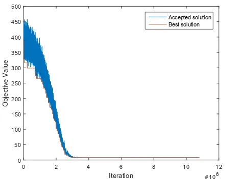
where the different settings result in a significant effect on the performance of SA and are shown in Figure 3.

Both configurations for solving the MAX-SAT problem produces the usual behaviour of a search method using SA as shown in Figure 3(a) and Figure 3(b). While the per-formance using both configurations is significantly different, the behaviour reflected in the traces are quite similar. The settings used for the domain-level strategy uses a low initial temperature (χ0= 5%)and a final temperature which means

that very few worse moves are still accepted at the end of the search. The cross-domain configuration on the other hand uses a very high initial temperature(χ0 = 90%)resulting in

a comparatively slow intensification of the search. Moreover, the low setting for the final temperature means that the search becomes stuck after ≈ 1/3rd of the search accepting only improving or equal quality moves.

The best configuration for solving the Bin Packing problem on the other hand (χ0 = 5%, tf inal = 0.00001) illustrates that the best performance is achieved by accepting as few worse quality moves as possible. The trace in Figure 3(c) shows a Bin Packing problem being solved by SA using this configuration. After an initial period of diversification, very few worse moves are accepted simulating an accepting improving or equals move acceptance scheme. Use of the cross-domain configuration can be seen in Figure 3(d). The high initial temperature results in a gross overshoot of the search resulting in wasted search time and ultimately poor per-formance. This is in contrast to the cross-domain configuration solving the MAX-SAT problem where this initial temperature setting appears balanced and highlights the sensitivity of SA not only to the parameter initialisation method, but also the move operators.

The Personnel Scheduling problem has a highly modal search landscape. Therefore, a random walk of the search space appears to perform the best with the domain-level parameter settings being set to their highest settings (χ0 =

(6)

Iteration #106

0 2 4 6 8 10 12

Objective Value

0 50 100 150 200 250 300 350 400

Accepted solution Best solution

(a) SA solving MAX-SAT problem instance ID 10 using theθDLparameter configuration,χ0= 5%andtf inal= 1.0.

Iteration #106

0 2 4 6 8 10 12

Objective Value

0 50 100 150 200 250 300 350 400 450 500

(b) SA solving MAX-SAT problem instance ID 10 using the θXD-Best parameter configuration,χ0= 90%andtf inal= 0.00001.

Iteration #105

0 0.5 1 1.5 2 2.5 3 3.5 4

Objective

Value

0.055 0.06 0.065 0.07 0.075 0.08 0.085 0.09 0.095 0.1

(c) SA solving Bin Packing problem instance ID 11 using theθDLparameter configuration,χ0= 5%andtf inal= 0.00001.

Iteration #105

0 0.5 1 1.5 2 2.5 3 3.5

Objective Value

0 0.1 0.2 0.3 0.4 0.5 0.6 0.7 0.8 0.9

(d) SA solving Bin Packing problem instance ID 11 using the θXD-Best parameter configuration,χ0= 90%andtf inal= 0.00001.

Iteration

0 1000 2000 3000 4000 5000 6000

Objective

Value

0 1000 2000 3000 4000 5000 6000 7000 8000

(e) SA solving Personnel Scheduling problem instance ID 5 using theθDL parameter configuration,χ0= 90%andtf inal= 10000.0.

Iteration

0 1000 2000 3000 4000 5000 6000 7000 8000

Objective

Value

0 500 1000 1500 2000 2500 3000 3500 4000 4500 5000

(f) SA solving Personnel Scheduling problem instance ID 5 using the

[image:6.612.320.557.58.234.2]

θXD-Bestparameter configuration,χ0= 90%andtf inal= 0.00001.

(7)

TABLE IV

MEAN AVERAGE,BEST RESULTS,AND STANDARD DEVIATION OF RESULTS OBTAINED BY EACH PARAMETER CONFIGURATION STRATEGY OVER31

TRIALS PER INSTANCE.

Problem θDL θXD-Best θXD-µ¯

Instance Mean Best SD Mean Best SD Mean Best SD

BP

7 0.0597 0.0558 0.0017 0.0681 0.0637 0.0024 0.0597 0.0558 0.0017

1 0.0328 0.0306 0.0017 0.0364 0.0351 0.0013 0.0328 0.0306 0.0017

9 0.0419 0.0394 0.0014 0.0437 0.0406 0.0015 0.0419 0.0394 0.0014

10 0.1221 0.1200 0.0010 0.1233 0.1206 0.0013 0.1221 0.1200 0.0010

11 0.0610 0.0576 0.0015 0.0680 0.0632 0.0019 0.0610 0.0576 0.0015

MAX-SA

T 3 7.81 4.00 2.02 15.42 10.00 2.59 14.06 5.00 3.47

5 13.74 7.00 3.55 34.48 16.00 10.53 33.84 16.00 11.13

4 7.65 3.00 2.36 18.42 8.00 7.40 16.45 5.00 7.42

10 8.87 4.00 2.28 17.81 9.00 2.99 14.45 9.00 2.34

11 8.26 7.00 0.86 10.35 7.00 1.25 9.87 7.00 0.99

PS

5 49.71 42.00 4.24 96.58 44.00 55.97 1020.61 289.00 366.41

9 51855.35 43315.00 4386.94 92249.65 79159.00 6530.84 99356.55 93175.00 3495.57

8 48566.10 45056.00 2012.74 51395.10 47258.00 2129.63 59961.19 57423.00 1019.24

10 1655.48 1530.00 75.27 1870.65 1654.00 147.74 2953.84 1920.00 771.37

11 474.61 392.00 51.51 1094.35 415.00 642.66 4434.61 1836.00 1268.87

FS

1 6282.61 6236.00 23.60 6287.87 6236.00 24.52 6282.77 6236.00 25.21

8 26815.16 26751.00 32.66 26827.03 26751.00 37.70 26817.35 26751.00 33.54

3 6347.32 6319.00 19.49 6349.61 6305.00 20.61 6350.00 6319.00 19.00

10 11406.13 11359.00 33.79 11405.23 11344.00 30.82 11403.45 11359.00 35.63

11 26666.61 26594.00 38.17 26666.97 26589.00 41.81 26663.19 26567.00 44.09

TSP

0 58777.11 55208.13 2347.26 59319.11 55573.38 2300.23 59217.79 55521.81 2389.84

8 2.506×107 _2.479_×₁₀7 _1.408_×₁₀5 _2.505_×₁₀7 _2.479_×₁₀7 _1.416_×₁₀5 _2.505×₁₀7 _2.479_×₁₀7 _1.419_×₁₀5

2 7936.98 7728.33 138.51 7974.66 7749.98 138.89 7972.13 7760.97 136.95

7 76982.33 75168.37 707.72 76617.48 74786.50 703.26 76569.54 74758.34 711.64

6 59621.38 57856.92 1037.75 59618.37 57783.36 1070.81 59611.85 57783.36 1067.06

VRP

6 324710.35 309246.58 6677.93 324400.15 309249.74 6630.66 325643.45 309290.71 6537.70 2 29523.78 25257.79 2022.90 29419.82 26042.13 2067.75 29447.22 25279.36 2087.32 5 347218.93 290779.35 84216.34 344662.76 282081.86 81847.89 563641.13 539264.30 11335.90 1 30565.62 24270.15 3815.53 30599.03 25336.76 3761.66 30564.85 24270.15 3816.14 9 389054.67 373573.02 7259.43 389027.63 373186.27 7260.28 390219.82 379735.24 6935.30

TABLE VI

RANKS OF THE OBTAINED DOMAIN-LEVEL PARAMETER CONFIGURATION COMPARED TO OTHER CONFIGURATIONS WITH RESPECT TO EACH

INDIVIDUAL TUNING INSTANCE.

Problem Domain Instance I Instance II

θDL(BP) 1 1

θDL(FS) 12 2

θDL(PS) 19 1

θDL(MAX-SAT) 1 2

θDL(TSP) 1 1

θDL(VRP) 1 3

D. Cross-domain Suitability

The parameter sensitivity combined with the characteris-tically different requirements for move acceptance favoured by some problems would suggest that SA is perhaps not the most suitable choice for the move acceptance component of a cross-domain search method, requiring intervention from domain experts for configuring its parameters. Further, the configurations obtained by the full factorial parameter tuning experiment for the domain-level strategy, θDL, was not the

top ranked configuration for both tuning instances within each problem domain. The ranks of the obtained configuration for both instances of each problem domain are shown in Table VI showing that parameter sensitivity remains an issue even at an intra-domain level.

V. CONCLUSIONS

In this paper, we investigated the plausibility of tuning a simulated annealing metaheuristic for cross-domain search. We showed that cross-domain parameter tuning then can be used to improve the cross-domain performance of the sim-ulated annealing based stochastic local search metaheuristic. Moreover, Taguchi orthogonal arrays can be used to reduce the computational budget of the tuning process without sig-nificantly affecting its performance cross-domain compared to if a full factorial design was used. Automatic parameter tuning methods [6] have been used previously to find the best parameter configurations for solving specific types of problems and parameter tuning is shown in this study to be of value for tuning a cross-domain search method. Hence, such methods should also be of value for cross-domain algorithms. The complete picture however shows that whilst the cross-domain tuning strategies investigated can be used to improve the cross-domain performance, they are still inferior to cross-domain-level tuning methods. Therefore, parameter tuning methods would have more benefit being applied at such a level and success at a cross-domain level is debatable.

(8)

move operators and for cross-domain search, means that the behaviour of the simulated annealing algorithm can vary sig-nificantly using the same parameter configurations. Moreover, some problems benefited from settings which detract from the characteristic behaviour of SA, instead simulating a random walk or acceptance of improving or equal moves only. Adap-tive variants of SA have been previously proposed such as Adaptive Simulated Annealing [36]. However by introducing such strategies, an increasing number of parameters are also introduced whose settings can effect the performance of the search method and drastically increases the complexity of such strategies. Moreover, such strategies tend to adapt to the search space rather than the characteristics of the problem being solved. Evidently, significant improvement can be realised through intelligent parameter setting strategies and/or adaptive methods.

In future work, the computational time budget for parameter tuning in cross-domain search methods can be reduced by us-ing the Taguchi orthogonal array design of experiments with-out significantly effecting its potential overall performance. Tuning the parameters for each domain however still remains the superior strategy highlighting the requirement for adaptive move acceptance methods which are less sensitive to their parameter settings for cross-domain search. The observations of the behaviour of the domain-level tuned Simulated Anneal-ing method across multiple problems also raises important questions for cross-domain search methods. How does the choice of move acceptance component effect the cross-domain performance of such algorithms, and which move acceptance method(s), if any, is (are) suitable for cross-domain search?

REFERENCES

[1] D. S. Garey, Michael R.; Johnson, Computers and Intractability: A Guide to the Theory of NP-Completeness. W. H. Freeman & Co., 1990.

[2] G. Ochoa and M. Hyde, “The cross-domain heuristic search challenge (chesc 2011),” 2011. [Online]. Available: http://www.asap.cs.nott.ac.uk/external/chesc2011

[3] E. K. Burke, M. Gendreau, M. Hyde, G. Kendall, G. Ochoa, E. ¨Ozcan, and R. Qu, “Hyper-heuristics: A survey of the state of the art,”Journal of the Operational Research Society, vol. 64, no. 12, pp. 1695–1724, 2013.

[4] K. S¨orensen and F. W. Glover, “Metaheuristics,” in Encyclopedia of operations research and management science. Springer US, 2013, pp. 960–970.

[5] F. Dobslaw, “Recent development in automatic parameter tuning for metaheuristics,” 2010.

[6] H. H. Hoos,Automated Algorithm Configuration and Parameter Tuning. Berlin, Heidelberg: Springer Berlin Heidelberg, 2012, pp. 37–71. [7] D. B. Gümüs, E. Özcan, and J. Atkin, “An investigation of tuning a

memetic algorithm for cross-domain search,” in2016 IEEE Congress on Evolutionary Computation (CEC), July 2016, pp. 135–142. [8] R. K. Roy,A primer on the Taguchi method. Society of Manufacturing

Engineers, 2010.

[9] S. Kirkpatrick, C. D. Gelatt, and M. P. Vecchi, “Optimization by simulated annealing,”Science, vol. 220, no. 4598, pp. 671–680, 1983. [10] M. Kalender, A. Kheiri, E. ¨Ozcan, and E. K. Burke, “A greedy

gradient-simulated annealing selection hyper-heuristic,”Soft Comput., vol. 17, no. 12, pp. 2279–2292, Dec. 2013.

[11] N. Metropolis, A. W. Rosenbluth, M. N. Rosenbluth, A. H. Teller, and E. Teller, “Equation of state calculations by fast computing machines,”

The Journal of Chemical Physics, vol. 21, no. 6, pp. 1087–1092, 1953. [12] M. Lundy and A. Mees, “Convergence of an annealing algorithm,”

Mathematical Programming, vol. 34, no. 1, pp. 111–124, 1986.

[13] R. Bai and G. Kendall,An Investigation of Automated Planograms Using a Simulated Annealing Based Hyper-Heuristic. Boston, MA: Springer US, 2005, pp. 87–108.

[14] M. Kalender, A. Kheiri, E. ¨Ozcan, and E. K. Burke, “A greedy gradient-simulated annealing hyper-heuristic for a curriculum-based course timetabling problem,” in 2012 12th UK Workshop on Compu-tational Intelligence (UKCI), Sept 2012, pp. 1–8.

[15] E. K. Burke and Y. Bykov, “The late acceptance hill-climbing heuristic,”

European Journal of Operational Research, vol. 258, no. 1, pp. 70 – 78, 2017.

[16] G. Ochoa, M. Hyde, T. Curtois, J. Vazquez-Rodriguez, J. Walker, M. Gendreau, G. Kendall, B. McCollum, A. Parkes, S. Petrovic, and E. Burke, “Hyflex: A benchmark framework for cross-domain heuristic search,” vol. 7245, pp. 136–147, 2012.

[17] M. Hyde, G. Ochoa, T. Curtois, and J. A. Vazquez-Rodriguez, “A hyflex module for the one dimensional bin packing problem,” School of Computer Science, University of Nottingham, Tech. Rep., 2010. [18] D. S. Johnson, A. Demers, J. D. Ullman, M. R. Garey, and R. L. Graham,

“Worst-case performance bounds for simple one-dimensional packing algorithms,”SIAM Journal on Computing, vol. 3, pp. 299–325, 1974. [19] ESICUP. (2011) European special interest group on cutting and packing

benchmark data sets. [Online]. Available: http://paginas.fe.up.pt/ esicup/ [20] M. R. Hyde. (2011) One dimensional packing benchmark data sets. [On-line]. Available: http://www.cs.nott.ac.uk/ mvh/packingresources.shtml [21] J. A. Vazquez-Rodriguez, G. Ochoa, T. Curtois, and M. Hyde, “A hyflex

module for the permutation flow shop problem,” School of Computer Science, University of Nottingham, Tech. Rep., 2010.

[22] M. Nawaz, E. E. E. Jr, and I. Ham, “A heuristic algorithm for the m-machine, n-job flow-shop sequencing problem,”Omega, vol. 11, no. 1, pp. 91 – 95, 1983.

[23] E. Taillard, “Benchmarks for basic scheduling problems,” European Journal of Operational Research, vol. 64, no. 2, pp. 278 – 285, 1993. [24] T. Curtois, G. Ochoa, M. Hyde, and J. A. Vazquez-Rodriguez, “A hyflex

module for the personnel scheduling problem,” School of Computer Science, University of Nottingham, Tech. Rep., 2010.

[25] A. Ikegami and A. Niwa, “A subproblem-centric model and approach to the nurse scheduling problem,”Mathematical Programming, vol. 97, no. 3, pp. 517–541, 2003.

[26] T. Curtois. (2009) Staff rostering benchmark data sets. [Online]. Available: http://www.cs.nott.ac.uk/ tec/NRP/

[27] M. Hyde, G. Ochoa, T. Curtois, and J. A. Vazquez-Rodriguez, “A hyflex module for the maximum satisfiability (max-sat) problem,” School of Computer Science, University of Nottingham, Tech. Rep., 2010. [28] CRIL. (2009) Sat competition 2009 benchmark data sets. [Online].

Available: http://www.cril.univ-artois.fr/SAT09/

[29] ——. (2007) Sat competition 2007 benchmark data sets. [Online]. Available: http://www.cril.univ-artois.fr/SAT07/

[30] J. Argelich, C.-M. Li, F. Manya, and J. Planes. (2009) Maxsat evalulation 2009 benchmark data sets. [Online]. Available: http://www.maxsat.udl.cat/

[31] G. Reinelt. (2008) Tsplib, a library of sample instances for the tsp. [On-line]. Available: http://comopt.ifi.uni-heidelberg.de/software/TSPLIB95/ [32] J. Walker, G. Ochoa, M. Gendreau, and E. K. Burke, “A vehicle routing domain for the hyflex hyper-heuristics framework,” in Proceedings of Learning and Intelligent Optimization (LION 2012), vol. 7219, 2012, pp. 265–276.

[33] SINTEF. (2011) Vrptw benchmark problems, on the sintef transport optimisation portal. [Online]. Available: http://www.sintef.no/vrptw [34] W. Ben-Ameur, “Computing the initial temperature of simulated

anneal-ing,”Computational Optimization and Applications, vol. 29, no. 3, pp. 369–385, 2004.

[35] S. Adriaensen, G. Ochoa, and A. Now´e, “A benchmark set extension and comparative study for the hyflex framework,” in Evolutionary Computation (CEC), 2015 IEEE Congress on. IEEE, 2015.