Using Petri Net modelling for a data driven approach to bridge management and safety

Using Petri-Net Modelling for a Data-Driven Approach to Bridge

Management and Safety

P. C. Yianni

Asset Management and Systems Assurance, Jacobs, Wokingham, Berkshire, RG41 5TU, United Kingdom.

L. C. Neves, D. Rama, J. D Andrews

Resilience Engineering Research Group, University of Nottingham,

Faculty of Engineering, University Park, Nottingham, NG7 2RD, United Kingdom.

R. Dean

Network Rail, The Quadrant:MK, Elder Gate, Milton Keynes, Buckinghamshire, MK9 1EN, United Kingdom.

ABSTRACT: Bridge portfolio managers have a difficult task managing a large, varied portfolio of aging assets

in a squeezed financial climate and on networks with increasing usage. Therefore, decision support tools are becoming more and more integral in managing portfolios of this scale. The model presented in this paper is designed to show a modern, data-driven approach to modelling which would sit as the base for the predictive module of a Bridge Management System (BMS). Extensive research has been carried out in this area however, it has usually resulted in bridge deterioration models; the approach taken in this research is to create a unified system model to encapsulate deterioration, inspection and maintenance to make a Whole Life-Cycle Costing (WLCC) model to offer new insight for bridge portfolio managers. The model in this research uses a Petri-Net (PN) approach which was decided upon as it is flexible enough to incorporate a complex deterioration module, calibrated with over a decade of historic inspection records, corporate policies regarding inspection and maintenance and even certain maintenance practices that are often overlooked. Using the model as a robust foundation, an investigation in the stressors which affect bridge deterioration is carried out. A low-cost, rapid approach to identifying which stressors are driving bridge deterioration is presented. The results indicate which stressors are a safety concern by accelerating the deterioration of bridge assets. Additionally, the results can be used in the PN model to create enhanced deterioration profiles. The resulting model is able to provide more accurate forward prediction capabilities of the assets condition over time, enhancing asset safety predicitons.

1 INTRODUCTION

Railway networks are often critical to the economy as they facilitate the movement of a both freight and commuters. This reliance creates an enormous amount of pressure on the railway and those who manage it. In the UK, a step change is due to oc-cur with the roll-out of the European Train Control System (ETCS) which will introduce moving block signalling, allowing trains to run closer together for greater network throughput (Technical Strategy Lead-ership Group (TSLG) 2012). Although this develop-ment will improve passenger experience, it increases the pressure on the backbone infrastructure. This re-search focuses on bridge management using the ex-ample of the UK railway network, which is owned

2 STOCHASTIC BRIDGE MODELS

A number of studies have been carried out to under-stand the deterioration behaviour of bridges. Stochas-tic models seem to be the preferred choice for modelling structural deterioration as they mimic the “micro-response” observed with structural deteriora-tion (Morcous, Lounis, & Cho 2010, Ditlevsen 1984), as well as the deterioration behaviour being natu-rally stochastic (Frangopol, Kallen, & van Noortwijk 2004).

The most popular technique for stochastic mod-elling of structural deterioration is the Markov model (Frangopol, Kallen, & van Noortwijk 2004). Jiang & Sinha 1989 was one of the first studies to use this ap-proach for bridge deterioration. The authors carried out a study in Indiana, USA, on a population of 5,700 bridges where 50 where chosen as random samples to calibrate the model with. The authors convert the condition of the assets to a scoring system used by the Federal Highway Administration (FHWA) which ranges from 0-9 with 0 being an element in poor con-dition and 9 being an element in a new concon-dition. The authors discuss the methodology which they use to calibrate the Markov Transition Probability Matri-ces (TPMs) using the historic condition data of the bridges. The authors found that the deterioration rate varied over the lifetime of the asset. The approach used in this study was utilised by the AASHTO in the creation of PONTIS, which is one of the most suc-cessful BMSs (Sobanjo & Thompson 2011).

Scherer & Glagola 1994 studied a population of 13,000 bridges in Virginia, USA. The authors de-velop a 7-state Markov model to predict the condi-tion of bridge assets. To increase the computacondi-tional efficiency, the authors group similar assets based on the structure type, age, number of spans, climate and loading. This reduced the number of Markov model

states from 713,000 _{to 7}216_{. The paper is pioneering}

in grouping assets by operational and structural at-tributes. Although there is little justification as to why those attributes were chosen, it demonstrates that cre-ating groups of assets with similar deterioration pro-files is a successful approach.

Agrawal, Kawaguchi, & Chen 2010 also utilised a 7-state Markov model to study a population of 17,000 bridges in New York, USA. The authors use his-toric data of bridge elements to calculate the effect of stressors using probabilistic lifetime distributions. One of their main comparisons was between bridges built with standard structural steel and those built with weathering steel. The results of the comparison was that the rates of deterioration were similar for the first 20 years of the assets life, but beyond that the weath-ering steel demonstrated lower levels of deteriora-tion than the standard steel. Investigating the stressors that affect bridge deterioration were key to this study, however the focus was mostly on the construction ma-terials rather than external environmental stressors.

Huang, Mao, & Lee 2010 focused on the external stressors that affect bridge deterioration on a popula-tion of 2,128 reinforced concrete structures in Taiwan. Analysis was carried out on the structures deteriora-tion behaviours to identify major and minor stressors by the types of defects that they cause. The authors identify traffic loading as a major stressor in the dete-rioration of the reinforcement bars and distance from the coast as a factor in causing spalling and fragmen-tation. Cracking seems to be one of the most prevalent types of defects as the results show that it is affected by 8 of the 10 stressors. The authors also identify that the peak monthly rainfall seems to be a major cause of concrete honeycombing. Finally, the distance from the coast is identified as a factor that affects structural deterioration, but was categorised as a minor stressor. However, the authors recognise that there were very few bridges in the population which would be classi-fied as coastal.

Le & Andrews 2014 created a PN-based WLCC bridge model using a modularised sub-net approach. A sub-net was created to model the deterioration of each major bridge component, each sub-net was then calibrated with historic bridge data. The authors fo-cused on metallic bridges with specialised sub-nets relating to the condition of the element coating and the condition of the underlying steel. The authors de-velop the model further to introduce Coloured Petri-Nets (CPNs) which enables a variety of features in-cluding the ability to perform state resets and enable tokens to hold tuple information about their respective bridge element. Monte Carlo (MC) simulation is per-formed using the model from which WLCC outputs are calculated. The paper demonstrated the flexibility of the PN approach and the suitability of CPNs to the application.

A number of studies have been evaluated which can be categorised into two main groups: 1) the studies which use historic bridge data to develop a bridge de-terioration or WLCC model and 2) the studies which analyse historic bridge data to try to deduce the fac-tors affecting bridge deterioration rates. The approach in this paper is to investigate the main external envi-ronmental factors affecting bridge deterioration and combine them into a WLCC model to understand the financial, operational and safety implications of the stressors over the lifetime of the asset.

3 CONDITION ASSESSMENT AND INDUSTRY

POLICIES

3.1 Condition Scores

A-G where A is no visible defect to G which is per-manent structural deterioration and from 1-6 where 1 is no extent to 6 where the defect extent is greater than 50% of the element surface area.

3.2 Condition Assessment

Condition assessments are used to schedule inspec-tions as well as decide upon maintenance acinspec-tions. SevEx is used to score each element during an inspec-tion, but these are then converted to a numerical Struc-ture Condition Marking Index (SCMI) afterwards. A good SevEx score would result in a high SCMI score e.g. an element in a new condition would be allocated an A1 SevEx score which would then be converted to an SCMI score of 100. The industry policies on future inspections and maintenance actions (Network Rail 2012a) describe SCMI thresholds which have been back-converted to SevEx scores for the purpose of this research to keep the method of condition assessment consistent.

3.3 Maintenance and Inspection Policies

The inspection frequency is dependant upon condi-tion, an element in a good condition (A1 to D2) would only need to be inspected every 12 years, an element in moderate condition (B6 to F3) would need to be inspected every 6 years and an element in poor con-dition (D6 to G6) would need to be inspected every 3 years (Network Rail 2012a).

Maintenance follows a similar pattern, with an ele-ment in good condition (B2 to D2) only being eligible for a Minor Repair, an element in moderate condition (B5 to F3) being eligible for a Major Repair. Elements in a worse state are deemed to be below the Basic Safety Limit (BSL) and would need to be replaced, relating to SevEx condition states D6 to G6. It should be noted that the A1 condition state is the only con-dition state which is not eligible for any maintenance (Network Rail 2010).

4 DATA SOURCES

A number of different data sources were used for this work, all of which were provided by NR. These in-clude the asset register, known as CARRS, the historic inspection data and the historic maintenance data, which is split between the Cost Analysis Framework (CAF) and MONITOR depending on the party that carried out the maintenance. In total the datasets cover 1998 to 2014 with inspection data for 25,949 bridges which breaks down into 273,427 major elements in-spected and 1,397,748 inspections of minor elements. Railway bridges are often comprised of either con-crete, masonry or metallic elements. Concrete bridges are becoming increasingly common which means the management of them is becoming more important

Figure 1: Basic PN components presented from left to right: 1) transition, 2) place, 3) marked place, 4) arc.

too. For this reason, concrete was chosen as the ma-terial type focused on in this research with the main girder elements chosen as the exemplar element. The dataset includes 4,434 concrete bridges, with 407,708 inspection of concrete main girders. Elements with a single inspection were discounted as at least two in-spection are required to calculate a condition delta.

5 PETRI-NETS

Although Markov models have traditionally been the preferred technique for modelling bridge deteriora-tion (Morcous 2006), they suffer from limitadeteriora-tions in-cluding: difficulties in calibrating the TPMs (Fran-gopol, Kallen, & van Noortwijk 2004), difficulty considering maintenance actions in the model (Mor-cous, Rivard, & Hanna 2002b, Robelin & Madanat 2007) and state based explosion issues (Agrawal, Kawaguchi, & Chen 2010, British Standards Institu-tion 2012). Although it is still understood that struc-tural deterioration is a stochastic process and there-fore, a stochastic model will best capture that be-haviour, (Frangopol, Kallen, & van Noortwijk 2004), the model enhancements presented in this research benefit from the flexibility of the PNs approach.

PNs are directed bipartite graphs created from places and transitions. Tokens occupy places and in-dicate the system state e.g. a token in the place ”Re-quires Maintenance” would indicate that the system is in a state requiring maintenance. Transitions move tokens between places and are calibrated with a fir-ing criterion known as a guard. For example, a transi-tion configured with a firing delay equal to the Mean Time to Repair (MTTR), could move a token from a “failed” place to a “working” place to model a sys-tem being repaired after a failure. Arcs are used to illustrate the dependencies between places and transi-tions. No two places or two transitions can be directly connected.

5.1 Coloured Petri-Nets

CPNs offer numerous features over simple PNs which are useful for modelling more complex systems (British Standards Institution 2004) including: 1) en-abling tokens to contain tuple information e.g. asset age 2) allowing the use of reset arcs which help sim-plify the model and 3) allowing more complex tran-sition guards including stochastic and programmatic guards (Jensen 1997).

Figure 2 shows a CPN where transitionΩis

β

α γ

δ Ω

Figure 2: CPN example with both inhibitor arc and reset arc.

to fire, it would remove all tokens in placeγ, this is

represented by the arc with cross.

6 CPN WLCC MODEL

The CPN model which has been developed is at a Tier 3 level i.e. it focuses on asset and sub-asset level. The model follows the modular sub-net approach which is common with this type of modelling technique. The modules connect in a cyclic way, broadly describing the life-cycle of an asset: starting with the compo-nent condition module which contains the deteriora-tion characteristics, through to the inspecdeteriora-tion module that triggers the maintenance module which, in turn, improves the condition of the bridge components in the deterioration module.

6.1 Component Condition Module

The component condition module, which can be seen in Figure 3, mimics the SevEx matrix described in Section 3. The decision to retain the 2-D condition matrix rather than convert to a linear scale, as is the de-facto standard (Cesare, Santamarina, Turkstra, & Vanmarcke 1992, Morcous 2006, Le & Andrews 2014, Network Rail 2010), was that: 1) structural de-fects have individualistic characteristics and convert-ing defects to a linear scale would involve weight-ings which introduces subjectivity and 2) the source inspection data uses the SevEx framework so using this data directly avoids any transformations which enables a more accurate calibration of the deteriora-tion profile.

In the module, transitions move tokens, represent-ing bridge components, between the condition states. Lifetime distributions could not be reliably calculated as the inspection data was of insufficient frequency. Therefore, the transitions are calibrated with a con-stant failure rate where failure is defined as mov-ing to a worse condition state. For example, in Fig-ure 3, there are two tokens representing two differ-ent bridge compondiffer-ents at differdiffer-ent levels of deterio-ration. These components are considered individually and move through the condition states independently i.e. triggered at different times, along different routes.

A1 B2 B3 C2 C3 Pending Condition Condition Determined Condition Change T10 T9 A1 B2 B3 C2 C3 Minor Repairs Major Repairs

Minor Repair Required

Major Repair Required

Replacement Required Intervention Planned

Between Inspection

During Inspection

Inspection Occurred

T13 T14 T15 T16

T11 T12 Between Intervention Intervention Commences T17 T18

Petri-Net for a Minor Element: Main External Girder (MGE), Concrete (C). All advanced transitions functions are represented with dashed arcs. WhereD/Prepresents a decision making probability transition that uses a ran-dom number to determine which probability the token is placed into e.g. (10%,80%,10%) if one of the inputs is designed to inhibit then the other options increase pro-portionately i.e. if the first 10% was inhibited then the options would become 80%+(80/90*10) = 88.89% and 10%+(10/90*10) = 11.11%;D/Mrepresents a transi-tion functransi-tion where a decision is based on marking, for instance it may determine the worst condition from the Sub-Minor Element conditions and places a token in the relevant place;Rrepresents a transition that is designed to reset a place or multiple places.

Transition Delay Type D/M D/P R T1 Stochastic No No No T2 Stochastic No No No T3 Stochastic No No No T4 Stochastic No No No T5 Stochastic No No No T6 Stochastic No No No T7 Stochastic No No No T8 Stochastic No No No

T9 Instant No No Yes

T10 Instant Yes No Yes T11 Conditional Yes No No T12 Small Delay (ε) No No Yes T13 Instant Yes Yes No T14 Instant Yes Yes No T15 Instant Yes Yes No T16 Instant Yes Yes No T17 Conditional Yes No Yes T18 Conditional Yes Yes Yes Figure 3: CPN component condition module. A reduced number

of condition states are shown for illustrative purposes. The total number of states is 31 which cover SevEx conditions A1 to G6.

A1 B2 B3 C2 C3 Pending Condition Condition Determined Condition Change

T1 T2

T3

T4

T5 T6 T7

T8 T10 T9 A1 B2 B3 C2 C3 Minor Repairs Major Repairs

Minor Repair Required

Major Repair Required

Replacement Required Intervention Planned

Between Inspection

During Inspection

Inspection Occurred

T13 T14 T15 T16

Between Intervention

Intervention Commences

T17 T18

Petri-Net for a Minor Element: Main External Girder (MGE), Concrete (C). All advanced transitions functions are represented with dashed arcs. WhereD/P represents a decision making probability transition that uses a ran-dom number to determine which probability the token is placed into e.g. (10%,80%,10%) if one of the inputs is designed to inhibit then the other options increase pro-portionately i.e. if the first 10% was inhibited then the options would become 80%+(80/90*10) = 88.89% and 10%+(10/90*10) = 11.11%;D/Mrepresents a transi-tion functransi-tion where a decision is based on marking, for instance it may determine the worst condition from the Sub-Minor Element conditions and places a token in the relevant place;Rrepresents a transition that is designed to reset a place or multiple places.

Transition Delay Type D/M D/P R T1 Stochastic No No No T2 Stochastic No No No T3 Stochastic No No No T4 Stochastic No No No T5 Stochastic No No No T6 Stochastic No No No T7 Stochastic No No No T8 Stochastic No No No T9 Instant No No Yes T10 Instant Yes No Yes T11 Conditional Yes No No T12 Small Delay (ε) No No Yes T13 Instant Yes Yes No T14 Instant Yes Yes No T15 Instant Yes Yes No T16 Instant Yes Yes No T17 Conditional Yes No Yes T18 Conditional Yes Yes Yes

Figure 4: The condition assessment module.

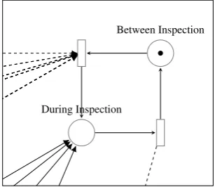
6.2 Condition Assessment Module

The condition assessment module schedules inspec-tions on the bridge components. The transition which initiates inspections is calibrated to fire in accordance with the industry guidelines for inspection (Network Rail 2012b). The industry policies describe how the condition relates to the frequency of inspection; the way this is represented in the model is with dashed arcs to the transition, which uses the marking of places to deduce the condition and then calculate the appropriate firing delay. The transition which fires to indicate the completion of an inspection is calibrated with the average length of time required for inspec-tions according to industry experts. Tokens in this module do not contain tuple information and simply indicate the system state by their presence/absence e.g. “between inspection”.

6.3 Rehabilitation Module

Fig-A1

B2 B3

C2 C3

Pending Condition

Condition Determined Condition Change

T1 T2

T3

T4

T5 T6 T7

T8

T10 T9

A1

B2 B3

C2 C3

Minor Repairs

Major Repairs

Minor Repair Required

Major Repair Required

Replacement Required Rehabilitation Planned

Between Inspection

During Inspection

Inspection Occurred

T13 T14 T15 T16

T11

T12

Between Rehabilitation

Rehabilitation Commences

Petri-Net for a Minor Element: Main External Girder (MGE), Concrete (C). All advanced transitions functions are represented with dashed arcs. WhereD/Prepresents a decision making probability transition that uses a ran-dom number to determine which probability the token is placed into e.g. (10%,80%,10%) if one of the inputs is designed to inhibit then the other options increase pro-portionately i.e. if the first 10% was inhibited then the options would become 80%+(80/90*10) = 88.89% and 10%+(10/90*10) = 11.11%;D/Mrepresents a transi-tion functransi-tion where a decision is based on marking, for instance it may determine the worst condition from the Sub-Minor Element conditions and places a token in the relevant place;Rrepresents a transition that is designed to reset a place or multiple places.

Transition Delay Type D/M D/P R T1 Stochastic No No No T2 Stochastic No No No T3 Stochastic No No No T4 Stochastic No No No T5 Stochastic No No No T6 Stochastic No No No T7 Stochastic No No No T8 Stochastic No No No T9 Instant No No Yes T10 Instant Yes No Yes T11 Conditional Yes No No T12 Small Delay (ε) No No Yes T13 Instant Yes Yes No T14 Instant Yes Yes No T15 Instant Yes Yes No T16 Instant Yes Yes No T17 Conditional Yes No Yes T18 Conditional Yes Yes Yes

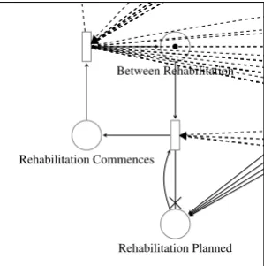
Figure 5: The rehabilitation module makes extensive use of CPN features to closely mimic the complex processes involved.

ure 5.

One major feature which was incorporated into the model required detailed expert judgement of the re-habilitation process. This situation occurs when the element has deteriorated into a worse state during the time between inspection and rehabilitation where the planned rehabilitation is no longer sufficient. This normally would only occur when then condition is near the boundary of rehabilitation actions or the ele-ment deteriorates particularly quickly. In Figure 5 this is represented by dashed arcs which are used to de-duce whether the rehabilitation action is still appro-priate based on the condition of the element. If the re-habilitation action is no longer appropriate the main-tenance teams would have to return to that element at a later date to carry out the appropriate rehabilitation action; this delays the repair, increases WLCC and in-creases pressure on maintenance teams.

6.4 Model Simulation and Outputs

With the use of stochastic transitions and complex guards in the CPN model, simple PN analytics are un-available which means the model must be simulated to understand its behaviour. A MC approach was used for this. The model outputs shown in this section re-sult from a simulation starting with a concrete beam element in an A1 condition over a 100 year period. To simulate an entire bridge asset, a token would be added for each bridge element. A single element was chosen for this example for illustrative purposes to avoid conflicting deterioration profiles and enable a visually clear behavioural trend. A total of 10,000 it-erations were carried out to ensure consistent results.

Figure 6 shows the condition of the element over time. The model, in this configuration, uses the stan-dard industry maintenance policies, described in Sec-tion 3. The condiSec-tion starts the simulaSec-tion with a de-terministic A1 condition, hence the high probability of residing in an A1 condition at the end of the first year. The downward slope of the condition contin-ues until the 12th year when an inspection and sub-sequent maintenance action take place, resulting in an uplift in condition. This process starts the saw-tooth

0 10 20 30 40 50 60 70 80 90 100

0 0.2 0.4 0.6 0.8 1

Years

Probability

A1 B2 B3 B4 B5 B6 C2 C3 C4 C5 C6 D2 D3 D4 D5 D6 E2 E3 E4 E5 E6 F3 F4 F5

Figure 6: Model simulation outputs showing the condition over time of a concrete girder element.

0 10 20 30 40 50 60 70 80 90 100 0

200 400 600 800 1,000 1,200

Years

Y

early

Cost

(

mu

)

Cost of Replacements Cost of Major Repairs Cost of Minor Repairs Cost of Inspections

0 10 20 30 40 50 60 70 80 90 1000 1,000 2,000 3,000 4,000 5,000 6,000 7,000 8,000

Cumulati

v

e

Cost

(

mu

)

Figure 7: Model simulation outputs showing the cost per year and cumulative cost over time of a concrete girder element.

cycle which continues over the life of the simulation describing the cycle of deterioration, inspection and maintenance.

Figure 7 shows a similar cycle, but from a finan-cial perspective. It can be seen that costs are only re-alised in years when inspections and maintenance oc-curs, which coincide with the condition uplifts seen in Figure 6. It should also be noted that when the main-tenance teams are required to return to an element, as described in Section 6.3, a second set of expendi-ture is realised, which can be seen in the figure as the smaller bars between the normal cycles.

7 INVESTIGATION INTO STRESSORS

The model presented so far considers generic bridge elements. From the literature reviewed, there seem to be a number of external environmental factors which can cause varying rates of deterioration in bridge elements. A number of studies have high-lighted that there are “other” factors which can con-tribute to bridge deterioration (Morcous, Rivard, & Hanna 2002a, Sobanjo 1997, Arditi & Tokdemir 1999), but to be able to investigate these a sufficiently large portfolio of bridges and wide enough dataset is required.

decided that retaining their format would avoid the need for weightings which can introduce subjectiv-ity. Therefore, an approach was developed which con-siders each of the 31 condition states as nodes with the “length” of the paths connecting the nodes to be equivalent to the Mean Time to Failure (MTTF), fol-lowing the approach of the deterioration module seen in Section 6.1. The most likely route from node to node through the network is the route which has he lowest MTTF. This allows the use of a classic rout-ing algorithm (Dijkstra 1959) to calculate the time it would take for an element to reach a condition requir-ing Major Rehabilitation or Replacement from its cur-rent condition.

The methodology would be to select an attribute which could be a contributor to structural deteriora-tion (e.g. amount of rainfall), and divide up the pop-ulation into equal groups e.g. structures exposed to

<700mm of rainfall per year or ≥700mm of rainfall

per year. Then calibrate a network diagram for each of the groups, calculating the shortest path for each condition state to the thresholds for Major Rehabili-tation or Replacement. The results can be compared as a quick visual indicator to identify if that particu-lar attribute may be a significant factor in structural deterioration.

7.1 Structure Configuration

Structural configuration was analysed to ascertain if it is a key factor in deterioration. Railway bridges are usually configured as either underline bridges or over-line bridges. Underover-line bridges carry the railway over obstacles, for example a roadway or river.

The population of underline and overline bridges were taken as two groups and analysed using the methodology described in the previous section. The results can be seen in Figure 8. The results give a visual indication that underline bridges deteriorate faster than overline bridges in general, which can be seen by the lower amount of time required to reach the threshold requiring rehabilitation. The difference highlighted by these results is most likely caused by the different stress profiles caused by the different types of vehicular traffic. The results indicate that these two bridge configurations should be treated as separate groups.

7.2 Distance to Sea

The distance of each bridge asset to the sea could be calculated using the assets location, provided in the CARRS dataset, with a shorelines database (National Oceanic and Atmospheric Administration (NOAA) 2015). The approach used in this paper was to divide the population of bridges from the coast inland i.e. a split at 10Km would create two groups of assets, bridges within 10Km to the sea and bridges 10Km or further from the sea. The population was split every

A1 B2 B3 C2 C3 C4 B5 B6 B4 C5 C6 D2 D3 D4 D5 D6

0 200 400 600 800

1,000

1,200

1,400

1,600

1,800

2,000

Initial Condition

MTTF

(Months)

Underline Bridges Overline Bridges

Figure 8: Analysis results of different bridge configurations to deteriorate to the Major rehabilitation threshold.

0 2 4 6 8 10 12 14 16 18 20 22 24 26 28 30

0

0.2

0.4

0.6

0.8

1

1.2

1.4

Bridge population Split atxkm

MTTF

normalised

to

Inland

Group

Inland Group Coastal Group

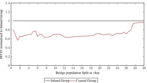
Figure 9: Bridge behaviour at different points from the sea, tested to a condition state requiring Major rehabilitation.

0.5Km up to 30Km inland. The groups would then be analysed with the methodology described in the pre-vious section.

The results can be seen in Figures 9 and 10. They show the inflection point between inland and coastal bridge behaviour. This was tested with a concrete girder element starting in an A1 condition and dete-riorating to a state requiring Major rehabilitation in Figure 9 and a state below the BSL, requiring ele-ment replaceele-ment in Figure 10. The results show that there is, in general, a significant difference in the de-terioration rate between the coastal and inland bridge groups with the MTTF being around 30% lower for the coastal group than the inland group. From these results, it can be seen that the distance to the sea is a factor affecting deterioration and the data suggests that the groups should be split with: 1) assets severely affected by the sea at 0-5Km, 2) assets in moderate exposure to the sea at 5-25Km and 3) assets with min-imal/no exposure to the sea beyond 25Km.

8 WLCC MODEL CONSIDERING STRESSORS

0 2 4 6 8 10 12 14 16 18 20 22 24 26 28 30 0

0.2

0.4

0.6

0.8

1

1.2

1.4

Bridge population Split atxkm

MTTF

normalised

to

Inland

Group

Inland Group Coastal Group

Figure 10: Bridge behaviour at different points from the sea, tested to a condition state below the BSL, requiring element re-placement.

practice is to embed the stressor information in the tuple of the bridge element token in the CPN model. The transitions are calibrated with each of the deteri-oration profiles based on the different stressors. The transitions use a stressor identifier in the token tuple to determine the appropriate firing delay to replicate the appropriate deterioration profile for an element exposed to that particular environmental factor.

A simulation has been carried out with a concrete girder element, starting in an A1 condition, inspected and maintained to the industry standard “managed” maintenance regime over a 100 year period. The re-sults have been summarised in Table 1. It can be seen that the generic deterioration profile (ID1), in which

stressor information is not considered, costs 7,900mu

over a 100 year period, which correlates to the model output seen in Figure 7. When running the simulation of the concrete girder element with different structure configurations, IDs 2 and 3 are the model WLCC out-puts, corresponding to overline and underline bridges. It can be seen that overline bridges cost considerably less than underline bridges. It should be noted that there are other structure configurations, but overline and underline bridges make up 94% of the portfo-lio. When simulating the concrete girder element on structures at different coastal proximities, the results are more divergent (IDs 4, 5 and 6). It can be seen that the WLCC of an inland bridge (ID6) is comparatively low whereas a structure which is closer to the sea (ID5) costs significantly more at 1.7 times that if ID1. Furthermore, structures that are very close to the sea, at maximum exposure to the saline atmosphere, cost almost twice the baseline WLCC seen in ID1. The variation in capital expenditure between these groups varies significantly and reveals a great deal to bridge portfolio managers.

As well as increased financial burden, factors which cause rapid deterioration can also cause issues with maintainability. This is evident when comparing Figures 8 and 8. In Figure 8, the deterioration rate is slower and so the delay time between inspection and maintenance is acceptable. However in Figure 8 the sawtooth curve begins to deviate suggesting that in-termediate rehabilitations are beginning to occur. The

Table 1: Stressor simulation WLCC results.

ID Structure

Configura-tion

Distance

to Sea

(km)

WLCC (nearest

100mu)

Relative Cost to ID 1

1 All 0 - Inf 7,900 1.000

2 Overline Bridges 0 - Inf 3,600 0.460

3 Underline Bridges 0 - Inf 7,100 0.906

4 All <5 15,100 1.918

5 All 5-25 13,700 1.736

6 All >25 2,800 0.355

situation under which this occurs is when the element has deteriorated further than expected on an initial rehabilitation attempt and so the maintenance teams must return. This causes an increase in WLCC, in-creases possession time of the asset and reduces main-tenance efficiency. The safety implications are that as-sets exposed to stressors which cause rapid deteriora-tion are more difficult to manage and therefore there is a higher likelihood of the element straying below the BSL.

0 10 20 30 40 50 60 70 80 90 100

0 0.2 0.4 0.6 0.8 1

Years

Probability

A1 B2 B3 B4 B5 C5 C6 D2 D3 D4 D5 D6 E3 E4 E5 E6 F4 F5 F6

Figure 11: Simulation of a concrete girder element<5Km from

the sea.

0 10 20 30 40 50 60 70 80 90 100

0 0.2 0.4 0.6 0.8 1

Years

Probability

A1 B2 B3 B4 B5 B6 C2 C3 C4 C5 C6 D2 D3 D4 D5 D6 E3 E4 E5 E6 F4 F5

Figure 12: Simulation of a concrete girder element>25Km from

9 CONCLUSION

The international standards for Asset Management (AM) discuss safety as a key aspect of good AM (In-ternational Organization for Standardization 2014). With an aligned AM strategy and objectives, under-standing the main risks that can cause an asset to breach the safety threshold can be avoided. In the work presented, a robust WLCC model was presented which develops new insight into how the policies which govern the management bridge assets affect them using historic condition data. Then an analy-sis into the main factors affecting deterioration allow bridge managers to understand the environmental fac-tors which are the highest risk of causing rapid dete-rioration. Finally, by combining the stressor analysis and the WLCC model, a financial, safety and main-tainability insight can be gained about the stressors, all of which can improve the AM understanding and help mitigate risks of assets falling below the BSL.

10 ACKNOWLEDGEMENTS

John Andrews is the Royal Academy of Engineering and Network Rail Professor of Infrastructure Asset Management. He is also Director of The Lloyds Reg-ister Foundation (LRF) Resilience Engineering Re-search Group at the University of Nottingham. Robert Dean is a Principal Engineer within the Safety, Tech-nical and Engineering team at Network Rail. Luis Canhoto Neves is an Assistant Professor in the Re-silience Engineering Research Group at the Univer-sity of Nottingham. Dovile Rama is the Network Rail Research Fellow in Asset Management. Panayi-oti Yianni is an Asset Management Consultant within Jacobs’ Asset Management and Systems Assurance team. The research was supported by Network Rail and the Engineering and the EPSRC grant refer-ence EP/L50502X/1. They gratefully acknowledge the support of these organizations.

REFERENCES

Agrawal, A. K., A. Kawaguchi, & Z. Chen (2010).

Deteriora-tion rates of typical bridge elements in New York.Journal of

Bridge Engineering 15(4), 419–429.

Arditi, D. & O. Tokdemir (1999). Comparison of Case-Based

Reasoning and Artificial Neural Networks.Journal of

Com-puting in Civil Engineering 13(3), 162–169.

British Standards Institution (2004). Systems and software en-gineering. High-level Petri nets. Concepts, definitions and graphical notation. Technical report, British Standards Insti-tution.

British Standards Institution (2012). Analysis techniques for de-pendability — Petri net techniques. Technical report. Cesare, M. A., C. Santamarina, C. Turkstra, & E. H. Vanmarcke

(1992). Modeling bridge deterioration with Markov chains.

Journal of Transportation Engineering 118(6), 820–833. Dijkstra, E. W. (1959). A note on two problems in connexion

with graphs.Numerische Mathematik 1(1), 269–271.

Ditlevsen, O. (1984).Probabilistic Thinking: An Imperative In

Engineering Modelling. Department of Structural Engineer-ing, Technical University of Denmark.

Frangopol, D. M., M.-J. Kallen, & J. M. van Noortwijk (2004). Probabilistic models for life-cycle performance of

deterio-rating structures: review and future directions. Progress in

Structural Engineering and Materials 6(4), 197–212. Huang, R.-Y., I.-S. Mao, & H.-K. Lee (2010). Exploring the

De-terioration Factors of RC Bridge Decks: A Rough Set

Ap-proach.Computer-Aided Civil and Infrastructure

Engineer-ing 25(7), 517–529.

International Organization for Standardization (2014). ISO 55001:2014 Asset management – Management systems – Requirements. Standard, Geneva, CH.

Jensen, K. (1997). A brief introduction to coloured Petri Nets. In

E. Brinksma (Ed.),Tools and Algorithms for the

Construc-tion and Analysis of Systems, Number 1217 in Lecture Notes in Computer Science, pp. 203–208. Springer Berlin Heidel-berg.

Jiang, Y. & K. C. Sinha (1989). Bridge service life

predic-tion model using the Markov chain.Transportation Research

Record(1223), 24–30.

Le, B. & J. Andrews (2014). Modelling Railway Bridge Asset

Management using Petri-Net Modelling Techniques. In

Pro-ceedings of the Second International Conference on Railway Technology: Research, Development and Maintenance. Morcous, G. (2006). Performance prediction of bridge deck

sys-tems using Markov chains.Journal of Performance of

Con-structed Facilities 20(2), 146–155.

Morcous, G., Z. Lounis, & Y. Cho (2010). An integrated system for bridge management using probabilistic and

mechanis-tic deterioration models: Application to bridge decks.KSCE

Journal of Civil Engineering 14(4), 527–537.

Morcous, G., H. Rivard, & A. Hanna (2002a). Case-Based Rea-soning System for Modeling Infrastructure Deterioration.

Journal of Computing in Civil Engineering 16(2), 104–114. Morcous, G., H. Rivard, & A. Hanna (2002b). Modeling bridge

deterioration using case-based reasoning.Journal of

Infras-tructure Systems 8(3), 86–95.

National Oceanic and Atmospheric Administration

(NOAA) (2015). GSHHG - A Global Self-consistent,

Hierarchical, High-resolution Geography Database.

https://www.ngdc.noaa.gov/mgg/shorelines/gshhs.html. Network Rail (2010). Handbook for the examination of

Struc-tures Part 11A: Reporting and recording examinations of

Structures in CARRS.NR/L1/CIV/006/11A.

Network Rail (2012a). Policy on a Page: Structures.

Network Rail (2012b). Structures Asset Management Policy and Strategy. pp. 219.

Robelin, C.-A. & S. M. Madanat (2007). History-dependent bridge deck maintenance and replacement optimization with

Markov decision processes. Journal of Infrastructure

Sys-tems 13(3), 195–201.

Scherer, W. & D. Glagola (1994). Markovian Models for Bridge

Maintenance Management.Journal of Transportation

Engi-neering 120(1), 37–51.

Sobanjo, J. (1997). Neural network approach to modeling bridge

deterioration. In Proceedings of the 1997 4th Congress on

Computing in Civil Engineering, June 16, 1997 - June 18,

1997, Computing in Civil Engineering (New York), pp.

623–626. ASCE.

Sobanjo, J. O. & P. D. Thompson (2011). Enhancement of the FDOT’s Project Level and Network Level Bridge Manage-ment Analysis Tools.