Contents lists available atScienceDirect
International Journal of Multiphase Flow
journal homepage:www.elsevier.com/locate/ijmultiphaseflow
Structures in gas–liquid churn flow in a large diameter vertical pipe
Safa Sharaf, G. Peter van der Meulen
1, Ezekiel O. Agunlejika, Barry J. Azzopardi
∗Faculty of Engineering, University of Nottingham, University Park, Nottingham NG7 2RD, UK
a r t i c l e
i n f o
Article history:
Received 22 June 2015 Revised 12 September 2015 Accepted 12 September 2015 Available online 23 October 2015
Keywords:
Gas–liquid flow Wire Mesh Sensor Conductance probes Churn flow Vertical pipe
a b s t r a c t
Gas–Liquid two phase co-current flow in a vertical riser with an internal diameter of 127 mm was investi-gated in the churn flow pattern. This paper presents detailed experimental data obtained using a Wire Mesh Sensor. It shows that the most obvious features of the flow are huge waves travelling on the liquid film. Wisps, large tendrils of liquid and the product of incomplete atomisation, which had previously detected in smaller diameter pipes, have also been found in the larger diameter pipe employed here. The output of the Wire Mesh Sensor has been used to determine the overall void fraction. When examined within a drift flux framework, it shows a distribution coefficient of∼1, in contrast to data for lower gas flow rates. Film thickness time series extracted from the Wire Mesh Sensor output have been examined and the trends of mean film thickness, that of the base film and the wave peaks are presented and discussed. The occurrence of wisps and their frequencies have been quantified.
© 2015 The Authors. Published by Elsevier Ltd. This is an open access article under the CC BY license (http://creativecommons.org/licenses/by/4.0/).
Introduction
Flow patterns in vertical pipes
Gas–liquid two-phase flow has many applications in the oil and gas, chemical and nuclear industries. When a two-phase mixture flows upwards in a vertical pipe, it is not possible to tell, a priori, how the phases are going to distribute themselves about the length and cross section of the pipe. Because of the infinite possibilities of distributions of the phases, researchers have tended to use flow pat-terns to describe the flows. These are broad descriptions of the flow. There is a consensus that the flow patterns for vertical flow are bub-bly, slug, churn and annular. Some groups add other patterns such as wispy annular and dispersed bubble to this list. The identification of when each flow pattern occurs is difficult to determine. Direct ob-servation through a transparent pipe section, particularly through a high speed camera, can allow visual and qualitative interpretation of the flow inside the pipe. However, this is very subjective, and in early projects such as byBennett et al. (1965), researchers formed a consensus through anonymous voting. Visual observations are also problematic, because the flow at the pipe wall is often obscured by bubbles or waves on wall films, particularly at higher velocities, meaning that it is difficult to see what is happening deep inside the pipe through this approach alone. A more objective approach is to gather signals from instruments and then interpret those signals
∗ Corresponding author. Tel.: +44 115 951 4160; fax: +44 115 951 4115.
E-mail address:[email protected](B.J. Azzopardi).
1
Present address: Atlantic Drilling Services, Amsterdam, the Netherlands.
quantitatively. What becomes obvious is that certain signatures are observed for particular types of flow, for example through the time series of void fraction and through the Probability Density Function (PDF). The PDF is a histogram of the occurrences of the different void fractions. This approach was used for example byJones and Zuber (1975)andCostigan and Whalley (1997). For bubbly flow there is a single peak at low void fraction. Slug flow contains two peaks (1st peak-liquid slug, 2nd peak – large gas bubble). Churn flow occurs at void fractions above 0.5–0.6, and it has a single peak with a tail extending down to lower void fractions. Annular flow has a single narrow peak at high void fractions of usually greater than 0.8. Much of the published work to date concentrates on small diameter pipes from 10 to 50 mm. This is in contrast with the larger diameter pipes which are more common in industry (i.e.,≥75 mm).
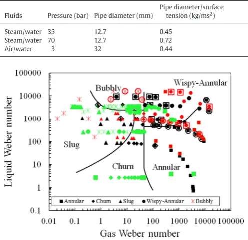
As noted above the early study of Bennett et al. (1965) gave a strong indication of difficulty of identifying which flow patterns were present at particular flow rates. Their experiments were on steam/water at 35 and 70 bar in a 12.7 mm pipe. They presented their results as plots of mass flux versus quality (steam mass fraction). Sub-sequently,Hewitt and Roberts (1969), who carried out experiments with air/water in a 32 mm diameter pipe at 3 bar, showed that if plotted as the momentum fluxes (the product of density,
ρ
i, times superficial velocity,uis, squared, withi=Gfor the gas and=Lfor the liquid) for the two phases their own data and those ofBennett et al. (1965)showed that the different flow patterns were found grouped in particular parts of the plot. Two questions arise from this: why do the different data sets agree and why are dimensional groups being employed rather than the usual dimensionless ones? The answer to the first question is that the momentum flux (or inertia force) is onehttp://dx.doi.org/10.1016/j.ijmultiphaseflow.2015.09.005
Table 1
Ratio of pipe diameter to surface tension for experiments ofBennett et al. (1965)and
Hewitt and Roberts (1969).
Fluids Pressure (bar) Pipe diameter (mm)
Pipe diameter/surface tension (kg/ms2)
Steam/water 35 12.7 0.45 Steam/water 70 12.7 0.72 Air/water 3 32 0.44
Fig. 1. Plot of liquid Weber number versus gas Weber number showing experimental
flow pattern data ofBennett et al. (1965)(Steam/water – 12.7 mm diameter pipes – pressure 35 bar (Black symbols) and 70 bar (Red symbols)) andHewitt and Roberts (1969)(Green symbols – air/water, 32 mm diameter pipe – pressure 4 bar) and transi-tion lines adapted fromHewitt and Roberts (1969).
of the most important forces in determining flow pattern. The answer to why these dimensional plots work so well is probably due to the ratio of pipe diameter,D, to surface tension,
σ
, for the three different conditions studied. These are listed inTable 1where it can be seen that two of the values are almost identical and the third is close. This could explain the agreement between the different data sets. It points to a way of obtaining non-dimensional plots. If the momentum fluxes are multiplied by pipe diameter and divided by surface tension, the graph would be the same but with stretched axes. The combinations (ρ
iu2isD/
σ
, whereiis either gas or liquid) are Weber numbers, the ratio of inertial to surface tension forces. In much of gas/liquid flow with low viscosity liquids these are the most important forces. For example, in one of the most important phenomena which occurs in annular flows, the atomisation of drops from the wall film, it is a We-ber numWe-ber which controls the size and probably the flux of drops produced. In slug flow, the production of small bubbles from the tail of the large bubbles is similarly the balance of inertial and surface tension forces. The data fromBennett et al. (1965)and fromHewitt and Roberts (1969)have been replotted in terms of liquid and gas We-ber numWe-bers inFig. 1. Here the 35 bar steam–water data are plotted in black, the 70 bar steam–water data in red and the 3 bar air–water data in green. Where there was more than one flow pattern selected in the voting process, symbols for both patterns are plotted. There is some, but not strong, agreement with the boundaries between flow patterns suggested byHewitt and Roberts (1969). This approach is for lower viscosity liquids. Obviously, a further refinement is required for more viscous liquids. [image:2.595.44.293.84.325.2]The fact that multiple flow patterns were selected for the same conditions might be taken as an indication of the difficulty of iden-tifying the features of the flow from photographs taken through the transparent pipe wall but also through a wavy film on the wall or a layer of bubbles at the wall. However, it might also be evidence that the flow pattern transitions are not sharp but there is a gradual shift from the characteristics of one flow pattern to those of another with
Fig. 2. Frequencies of slugs/huge waves/disturbance waves reported bySekoguchi and
Mori (1997). Pipe diameter=25.8 mm, pressure=2 bar, liquid superficial velocity=
0.4 m/s.
characteristics of both occurring simultaneously under some con-ditions. Further evidence of this gradual transition comes from the work ofSekoguchi and Mori (1997)who interrogated the gas–liquid flows using multiple probes, either axially or about a cross-section of the pipe. From the time resolved signals of all these probes they were able to identify individual examples of the structures which characterise each flow pattern. They found that more than one type of structure can occur at combinations of gas and liquid flow rates. Fig. 2illustrates the frequencies of the periodic structures that they obtained. The frequencies fall and rise systematically with increasing gas superficial velocity with regions where more than one structure is present. A similar plot, but for the lower superficial of 0.1 m/s was presented byHernandez Perez et al. (2010).
Characteristics of individual flow patterns
Fig. 3.Effect of pipe diameter on void fraction in liquid slug and in Taylor bubble re-gion. All cases are for air-water and are taken from the same overall average void frac-tion. FromOmebere-Iyari (2006). Data from:Omebere-Iyari and Azzopardi (2007)– 5 mm;Cheng et al. (2002)– 29 mm;Kaji et al. (2009b)– 52 mm;Kaji (2008)– 70 mm;
Cheng et al. (1998)– 150 mm.
clear bullet shape. Indeed, at diameters>100 mm, there does not ap-pear to be any slug flow. A reason for this can be seen inFig. 3where data from air–water experiments for the void fraction in the liquid slug and that in the Taylor bubble region from different pipe diame-ters, but for the same mean void fraction, have been plotted. The void fraction in the liquid slug increases from∼zero because increased entrainment of gas from the tail of the Taylor bubble as the pipe di-ameter increases. At smaller pipe didi-ameters, the void fraction in the Taylor bubble region is approximately constant but beyond∼100 mm it decreases due to bubbles passing through the slug and into the film surrounding the Taylor bubble making it knobbly and different from the idealised bullet shape. At the larger pipe diameters there are still periodic structures whose velocities, obtained from cross-correlation of time series from two probes at different axial locations show the same trend with flow rates as noted above.
Inannularflow, the liquid travels partially as a film on the channel walls with the rest being carried by the gas as entrained drops. The drops are created from waves of the film interface and after trans-portation by the gas redeposit onto the film either ballistically, due to the momentum they obtained on creation, or by a diffusion-like pro-cess due to the turbulence in the gas. The fraction of liquid depositing by either one of these mechanisms can vary between 0 and 1.
There have been a number of mechanisms proposed for the tran-sition from slug to churn flow as the gas flow is increased.Nicklin and Davidson (1962)identified that the difference between the down-wards velocity of the falling film surrounding the Taylor bubble and the upwards velocity of the gas in the bubble could arrive at the con-ditions of flooding, i.e., the instability when the liquid is stopped or even forces upwards. This has been taken up by others;McQuillan and Whalley (1985)followed this suggestion and produced a tran-sition criterion. The approach was modified byJayanti and Hewitt (1992)who argued that, since there is a significant effect of film length on the flooding point in counter-current flow, the length of the Taylor bubbles should be taken into account. They used their own correlation to include this effect.Watson and Hewitt (1999)have compared the predictions of the correlations ofMishima and Ishii (1984), McQuillan and Whalley (1985), Brauner and Barnea (1986) andJayanti and Hewitt (1992)with some extensive air/water data at 1.2, 3 and 5 bar in a 32 mm pipe. They found that only the equation of Jayanti and Hewitt (1992)predicts the correct trend. Support for the importance of flooding in the slug/churn transition has been provided byKaji et al. (2009a). They measured void fraction time series from several, closely-spaced conductance probes. By selecting that data
from the Taylor bubble sections and employing a cross-correlational analysis, they identified that there were waves with both upwards and downwards velocities present for a set of flow conditions, an oc-currence that would be expected around flooding.Taitel et al. (1980) consider that churn flow is an entry effect associated with plug flow and have produced a model including a length effect. This approach implies that for infinitely long pipes only bubble, slug and annular flow should occur and thus a direct transition mechanism between plug and annular flows is required. However, in slug flow the film can be flowing downwards whilst in annular flow it flows upward, so an intermediate state might be expected between the film down-flow and updown-flow, particularly from the evidence provided by flooding experiments. For this reason the Taitel et al.’s approach is not consid-ered to be appropriate.Mishima and Ishii (1984)postulated that the transition between slug and churn flow results from a void fraction limitation. They calculated the mean void fraction over the length of a gas slug by a potential flow analysis and the mean void fraction over the total slug unit from a drift flux analysis. The transition was de-fined as the condition at which the void fractions were equal. Though their transitions showed good agreement with experiment it is not considered reliable because: (i) there is an apparently incorrect ap-plication of Bernoulli’s equation; and (ii) they assumed that the plug length is determined when the film thickness reaches that calculated for a falling laminar film and that the length of the liquid slug is ap-proximately zero. Both these are unreasonable assumptions and this approach is not considered suitable.Brauner and Barnea (1986)also used a limiting void fraction approach, and proposed that slug flow would change to churn flow when the void fraction in the liquid slugs between the Taylor bubbles became equal to the maximum packing void fraction for a cubic lattice of equal sized spherical bubbles (de-fined above as
ε
g=0.52). Thus the transition line can be obtained replacingε
g=uGs/(uGs+uLs)=0.52.Dukler and Taitel (1977) sug-gested that the transition might be caused by the length of the liquid slug separating two Taylor bubbles becoming too short and the wake behind the Taylor bubble breaking up the liquid slug. The findings of Pinto et al. (1998)give support to this concept. They reported that the second of two Taylor bubbles would accelerate into the tail of the first if liquid slug between them was less than 5 pipe diameters long.Churn flow
There is also a lack of agreement as to what constitutes churn flow. It is fairly certainly a gas continuous flow. There is growing agreement that there are huge waves present and some of the liquid is carried as drops.Sekoguchi and Mori (1997)andSawai et al. (2004)using measurements from their multiple probes (92 over an axial length of 2.325 m) obtained time/axial position/void fraction information. From this they were able to identify huge wave from amongst distur-bance waves and slugs. They classified individual structures as huge waves from their size together with the fact that their velocities de-pended significantly on the corresponding axial length. This was in contrast to disturbance waves where the velocity of individual waves only increased slightly with the axial extent of these waves. They also found that the frequency of huge waves first increased and then de-crease with increasing gas superficial velocity. Similarly, their veloc-ities were found to deviate from the line for slug flow velocveloc-ities and pass through a maximum and then a minimum.
Fig. 4. Measured values of entrained fraction covering the churn and annular flow pat-terns.●Verbeek et al. (1992), pipe diameter=50 mm, liquid superficial velocity=0.01 m/s;◦Westende et al (2007), pipe diameter=50 mm, liquid superficial velocity=0.01 m/s;Westende et al (2007), pipe diameter=50 mm, liquid superficial velocity=
0.04 m/s;Verbeek et al. (1992), pipe diameter=100 mm, liquid superficial velocity
=0.01 m/s;Verbeek et al. (1993), pipe diameter=100 mm, liquid superficial veloc-ity=0.05 m/s;♦van der Meulen (2012), pipe diameter=127 mm, liquid superficial velocity=0.04 m/s. Modelling▬▬pipe diameter=50 mm, liquid superficial velocity
=0.01 m/s;̶̶ ̶̶̶ ̶̶ ̶̶̶ ̶̶pipe diameter=100 mm, liquid superficial velocity=0.01 m/s;●●●●●
pipe diameter=100 mm, liquid superficial velocity=0.05 m/s; ———– pipe diameter
=127 mm, liquid superficial velocity=0.04 m/s.
The diameter of the sampling probe facing upstream into the flow was 6.35 mm which means that waves higher than 6.4 mm would be sampled.Wang et al. (2013b)have shown evidence of wave heights much greater than this value. If porous wall film removal devices are employed, it is noted that the momentum of the liquid in the huge waves could carry them past the device and that liquid would not be sucked off so giving an over large value of entrained fraction. Another possible technique is to utilise Phase Doppler Anemometry which uses the scattering of laser light to obtain information on the velocity, size and number flux of drops. The technique breaks down at higher drop concentrations as the plethora of drops can obscure the laser beams invalidating the measurements. These problems are less at very low liquid flow rates. Such data can be examined to give indication of trends. Examples of such data are presented inFig. 4 where the entrained fraction is plotted against a dimensionless gas velocity defined asuGs{
ρ
G/[(ρ
L-ρ
G)gD]}. The data come from the work ofVerbeek et al. (1992, 1993), who used a porous wall film take of approach on 50 and 100 mm diameter pipes at a liquid superfi-cial velocities of 0.01 and 0.05 m/s,Westende et al. (2007), who used Phase Doppler Anemometry on a 50 mm diameter pipe at liquid su-perficial velocities of 0.01–0.04 m/s, andvan der Meulen (2012)who employed the same technique on a 127 mm diameter pipe with liq-uid superficial velocities≤0.04 m/s. The data are plotted against di-mensionless gas velocity, a form of Froude number as in churn flow the important forces are inertia and gravity. It is recognised that the surface tension force can also be important. However, the data con-sidered here are all for air–water and so surface tension is essentially a constant. It can be seen that in the churn flow region the entrained fraction increases as the gas superficial velocity decreases. The posi-tion at which this increase takes place commences at higher gas ve-locities the larger the pipe diameter. Also shown in the figure are the predictions from the model ofAhmad et al. (2010). This is an empir-ical correction for churn flow to the model developed byHewitt and Govan (1990)for annular flow. That employs equations for the rates of entrainment and deposition which are assumed equal to each other at equilibrium. The combined equation is then solved for entrained fraction. The correction proposed by Ahmad et al. assumes that churn flow occurs forug∗<1, has the form 9.73−8.73ug∗and is applied to the expression for entrainment rate. It is seen that though it gives therise shown by the experimental data in churn flow, the exact values are not well predicted.
Models of the waves in churn flow have been published by Barbosa et al. (2001), Da Riva and del Col (2009)andWang et al. (2012, 2013a, 2013b). They focused on the entry point of liquid through a porous wall section and modelling the growth of waves.
Under some conditions, churn flow exhibits flow reversals in the liquid layer near the wall. This was visualised byHewitt et al. (1985)by using refractive index matching between the tube wall and the fluid to minimise optical distortion. A photochromic dye was dissolved in the liquid phase which could be activated using a pulsed laser beam to give a line in the liquid. In contrast to annu-lar flow where the line was always distorted upwards, in churn flow it was seen that the line was distorted downwards in the film be-tween waves and upwards when a wave passed up the pipe. Sup-port for this observation has come from the work ofZangana and Azzopardi (2012)who made measurements of wall shear stress us-ing a film mounted hot film probe whilst simultaneous measurus-ing the film temperature upstream and downstream of the probe with flush mounted resistance thermometers. They found that in churn flow shear stresses that were both positive and negative were present indicating reversal of flow.
Wispy-annular flow
Another flow pattern that is identified by some researchers is wispy-annular flow. It was first reported byBennett et al. (1965)who noted that if the liquid flow rate is increased in annular flow, large liquid objects may be observed within the gas core. These have been termed ‘wisps’. This has been classified as a separate flow pattern byHewitt and Roberts (1969). It is noted that observation or pho-tography through the transparent pipe wall to capture those struc-tures that occur in the centre of the pipe can be made difficult by the liquid film on the pipe wall which at the flow rates of interest can have a wavy interface and contain bubbles and so obscure the view. X-ray photography experiments were more successful. An example of such a photograph is shown inFig. 5(a).Prasser et al. (2002)who employed a Wire Mesh Sensor reported similar structures occurring in a 51 mm diameter pipe at liquid and gas superficial velocities of 1 m/s and 10 m/s respectively. From the output of a Wire Mesh Sen-sor,Hernandez Perez et al. (2010)recently reported the existence of similar structures in a vertical air–water flows in a 67 mm diameter pipe at atmospheric pressure,Fig. 5(b). They studied a mixture air and water and the flow rates corresponding to this image were liquid and gas superficial velocities of 0.25 m/s and 5.7 m/s respectively.
Sekoguchi and Mori (1997)applied a probe consisting of 257 nee-dles facing upstream in a 26 mm diameter vertical pipe. An electrical current was applied between each needle and the pipe wall and the outputs were used to determine the distribution of the phases about the pipe cross-section resolved in time at a frequency of 400 Hz. An example of their results is reproduced inFig. 6and shows elements protruding into the gas core which can be identified as wisps.
Hawkes et al. (2000)used optical detectors to study the pulsa-tions in the flow. They found two peaks in the power spectral den-sity of the signal fluctuations. These were attributed to disturbance waves and wisps. Confirmation of this was obtained when they re-peated the measurements after removing the wall film through a sec-tion of porous wall and only the peak corresponding to the wisps was observed.
Fig. 5. Wisps: (a)Hewitt and Roberts (1969), x-ray photography. Pipe diameter=
32 mm, gas superficial velocity=3.1 m/s, liquid superficial velocity=2.8 m/s; (b)
Hernandez-Perez et al. (2010), Wire Mesh Sensor. Pipe diameter=67 mm, gas super-ficial velocity=5.7 m/s, liquid superficial velocity=0.25 m/s.
be present and gives support to the source of wisps being incomplete atomisation, i.e., they are ligaments drawn out from waves on the film interface.
The number of publications on churn flow has increased recently. Apart of the modelling papers ofBarbosa et al. (2001), Da Riva and del Col (2009)andWang et al. (2012, 2013a, 2013b), those byHernandez Perez et al. (2010), Szalinski et al. (2010)andParsi et al. (2015a, 2015b) report on the application of Wire Mesh Sensors to air/liquid flows in 67 or 76 mm diameter vertical pipe. All used air as the gas. Hernan-dez Perez et al. and Parsi et al. employed water as the liquid whilst Szalinski et al. used a silicone oil (liquid viscosity=5 mPa s, surface tension=0.02 N/m). Parsi et al. also studied aqueous CMC solutions with viscosities 10 and 40 times that of water. Their gas and liquid flow rates, in terms of superficial velocities, were in the ranges of 3 to 38 and 0.1 to 0.76 m/s respectively. They all reported the pres-ence of huge waves. They used the output of Wire Mesh Sensors to provide qualitative and quantitative information about the flow. Waltrich et al. (2013)examined bubbly, slug, churn and annular flow in a 48 mm diameter riser. They utilised a pair of intrusive needle probes which extended from the wall towards the pipe centre. By measurement the resistance between them they obtained time series information about the void fraction in their pipe.
Structure of the paper
This paper reports on air/water churn flow in a large diameter ver-tical pipe employing Wire Mesh Sensors and other instrumentation. It presents the structures observed and then uses quantitative infor-mation on the flows examining it using:
1. a one dimensional approach;
2. a two and three dimensional approach.
In particular it identifies when wisps occur and on their frequen-cies of occurrence.
Fig. 6. Cross-sections of huge waves showing protrusions, i.e., wisps. Obtained bySekoguchi and Mori (1997)using SS=CHOP probes, pipe diameter=25.8 mm, gas superficial
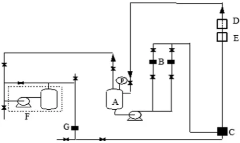
[image:5.595.91.492.451.724.2]Fig. 7. Experimental facility and instrumentation. A: liquid storage tank/separator; B: liquid flow meters; C: gas-liquid mixer; D: Wire mesh Sensor; E: conductance probes; F: compressor; G: gas flow meter.
Experimental arrangements
Experimental facility
The experiments conducted in the present study were carried out on a closed loop facility with a vertical riser (127 mm diameter pipe, 11 m tall). A schematic of the rig is given in Fig. 7. Air was pro-vided by the pair of liquid ring pumps acting as the compressor (each with a 55 kW electric motor), it is metered a Küppers turbine flow meter (35–1030 m3/h) and fed into the bottom of the riser where it was mixed with water drawn from the combined liquid storage tank/phase separator and metered by one of a pair of Küppers turbine flow meters mounted in parallel (0.006–0.06 and 0.04–0.5 m3/min). The uncertainties associated with the flow meters were±0.6% for the gas and±0.5% for the liquid. The mixer was in the form of an annu-lus, the gas was introduced through a centre pipe whilst the liquid entered through the annulus. From the top of the riser the two-phase mixture was returned to the phase separator, the gas returning to the compressor. The system pressure was kept constant at 3 bar (abs) (gas density=3.6 kg/m3). The superficial velocities studied were 3– 16.5 m/s for the gas and 0.001–0.65 m/s for the liquid. The riser was provided with a Wire Mesh Sensor, placed at a height of 9.3 m from the mixer, and three conductance probes positioned 7.96, 8.06 and 8.32 m downstream of the mixer.
A large number of runs were carried out during which the Wire Mesh Sensor and the conductance probes were triggered simulta-neously. A selection of runs was repeated to check for reproducibil-ity. A good consistent accuracy demonstrated.Hewakandamby et al. (2014), using the facilities described here made measurements with the Wire Mesh Sensor positioned at 35.4 and 82.7 pipe diameters from the mixer with over a range of gas and liquid superficial veloc-ities. Only at liquid superficial velocities below 0.03 m/s were there any significant differences between the mean void fractions obtained from the two stations implying that for higher liquid superficial ve-locities the flow was very close to being fully developed at the top station.
Instrumentation
The Wire Mesh Sensor employed is based on the methodology of Prasser et al. (1998) and was designed and manufactured by Helmholtz-Zentrum Dresden-Rossendorf (HZDR). It has two orthog-onal arrays of 32 very fine steel wires (0.1 mm diameter) stretched across parallel chords of the pipe cross-section. This gives a resolution of approximately 4×4 mm2. The transmitting and receiving wires are separated by a small axial gap of 2 mm and measurements are taken at each crossing point of the wires. During the measuring cy-cle, one of the transmitter wires is activated successively while all the
others are kept at ground potential. All the receiver wires are sampled in parallel. The collected raw data are processed off line. Details are provided inAzzopardi et al. (2010).
The Wire Mesh Sensor instrumentation has been tested by mak-ing simultaneous measurements with it and with Electrical Capaci-tance Tomography byAzzopardi et al. (2010)and with
γ
-ray absorp-tion bySharaf et al. (2011). Good agreement between the instruments was achieved in both cases, usually within 2%. In the comparisons with Electrical Capacitance Tomography, excellent agreement was achieved between the two methods in both the overall (cross-section and time-averaged) void fraction and the time-varying time series of cross-sectionally averaged void fraction. Most recently,Zhang et al. (2013)have made simultaneous measurements using a Wire Mesh Sensor device placed 8 mm downstream of a plane at which an ultra-fast x-ray tomography system was operating. Radial profiles of time averaged gas fraction distributions show good agreement between both techniques.Theconductance probes consisted of two metallic rings (3 mm thick) separated by a 25 mm thick acrylic resin ring mounted flush with the wall of the test section. An A.C. voltage (20 kHz) was im-posed across the two rings and the current passing was obtained and used to determine the resistance of the gas-liquid mixture and hence its void fraction. The current (determined from the voltage across a resistor mounted in series with the rings) exhibits a non-linear rela-tionship with void fraction and so they require calibration. For Churn and Annular-type flows this is carried out by placing non-conductive cylinders inside the pipe and filling the annulus between the cylinder and pipe wall with the conductive liquid.
The conventional probe calibration approach usually assumes that the liquid film is totally liquid. In reality, in gas–liquid churn and annular-type flows, the continuous trapping and folding actions of the large waves at the interface transport gas bubbles into the liquid film. The presence of a considerable amount of bubbles in the liquid film was reported in both air–water horizontal and vertical annular-type flows byJacowitz and Brodkey (1964), Hewitt et al. (1990)and Omebere-Iyari (2006).Rodriguez and Shedd (2004)quantified the bubble size distribution, bubble mean diameter and bubble number concentration in the wall film of a horizontal annular flow in a pipe of 15.1 mm diameter. They reported that bubbles had an exponential distribution of sizes with average diameters between 15% and 45% of the film thickness at gas superficial velocities ranging from 28 to 65 m/s and liquid superficial velocities from 0.019 to 0.14 m/s. Around 100 bubbles/cm2exist in the wall film at a gas superficial velocity 28 m/s.
To check the uncertainty introduced by the presence of bubbles, a new calibration approach was devised. In order to simulate gas bub-bles in the liquid film during annular-type flows, spherical glass beads were used, inserted into the liquid layer between the pipe wall and the inserted cylinder. The effect of the beads (bubbles) could give an uncertainty in the film thickness of 20%. It is noted this is an upper limit when the gap is full of beads. However, the large uncertainty means that it might not be appropriate to use it for void fraction and film thickness measurements. However, huge waves are still seen in the Conductance Probe output, the time traces from two, axially-displaced of the instruments can be cross-correlated to provide a de-lay time from which wave velocities can be extracted.
Results and discussion
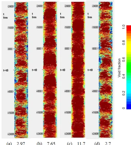
Fig. 8. Sectional view of flow in the pipe for different gas superficial velocities. (in m/s) Liquid superficial velocities are 0.66 m/s for (a) to (c) and 0.56 m/s for (d).
and space averaged) void fraction; (3) time series of cross-section av-eraged void fraction, velocities and frequencies of the periodic struc-tures found in the flow and (4) the flow rates at which wisps occur and their frequencies.
Interfacial structures
Images made up of the time sequences of the phase distribution across a pipe diameter have been created. Examples from four gas velocities are shown below inFig. 8(a–d). The information is held in the form of pixels of 4×4 mm. These are coloured according to the amount of liquid within that area. In these, the reddish-brown colour represents 100% gas whilst blue is 100% liquid. Light blue, or-ange and yellow represent intermediate values according to the scale inFig. 8. When used in conjunction with the time series of
cross-sectional phase distributions, it is seen that the flow pattern is essen-tially churn flow. There are very obvious regular huge waves. These are most evident for the lower gas and highest gas flow rates. The peaks of the waves can penetrate up to 1/3 of the pipe diameter from the wall. The waves are not totally symmetrical and though they oc-cur on both sides of the pipe at approximately the same time, the two sides can have significantly peak thicknesses. As the gas superficial velocity increases the peak heights decrease as seen inFig. 8(a–c). This aspect will be discussed quantitatively in below.
di-Fig. 9. Illustration of a wisp in the gas core of the pipe in the present experiments. Gas superficial velocity=3 m/s, liquid superficial velocity=0.265 m/s.
ameter. Given the solidity of the liquid body with these dimensions, use of the term wisp, with its connotations of lightness, must be con-sidered poetic.
[image:8.595.314.559.57.223.2] [image:8.595.66.272.59.542.2]Mean void fraction
Fig. 10 presents the (time and cross-sectionally) averaged void fraction obtained from the Wire Mesh Sensor measurements. The data was obtained for a series of liquid superficial velocities (0.053-0.66 m/s) and gas velocities between 3 and15 m/s. The figure illus-trates that the void fraction depends on both gas and liquid flow rates but that the dependency is not strong. This is not unexpected from published data in this range of flow rates.
[image:8.595.315.559.257.417.2]To quantify the relationship between void fraction and the phase flow rate the Drift Flux approach, proposed by
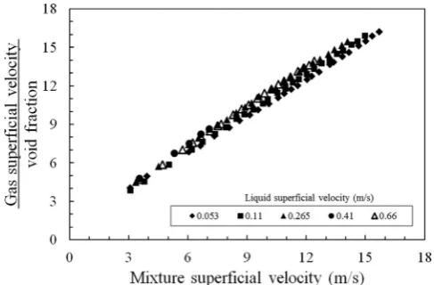
Fig. 10. Effect of gas and liquid superficial velocity on time and cross-section averaged
void fraction.
Fig. 11.Plot of gas velocity (gas superficial velocity/void fraction) versus mixture
[image:8.595.312.562.474.547.2]velocity.
Table 2
Parameters for the linear drift flux fits. Liquid superficial
velocity (m/s)
Distribution coefficient
Drift velocity (m/s)
Regression coefficient 0.053 0.96 0.99 0.9995 0.11 1.01 0.72 0.9998 0.265 1.01 1.28 0.999 0.41 1.04 1.23 0.9992 0.66 1.05 0.97 0.9996
Zuber and Findlay (1965) and employed by Sawai et al (2004) for churn flow, has been followed.Fig. 11shows a plot of gas velocity (gas superficial velocity divided by void fraction) against mixture velocity (the sum of the superficial velocities of the gas and the liquid,um). A linear relationship is expected as seen inFig. 11. The co-efficients of the linear equation and regression coefficient (a measure of the goodness of fit) are tabulated inTable 1. The values are close to those reported bySawai et al. (2004), .i.e., 0.99, 0.83 for liquid superficial velocities<0.2 m/s and 1.07, 0.74 for liquid superficial velocities≥0.2 m/s. These values are slope and intercept respectively in both cases(Table 2).
Fig. 12. Plot of gas velocity (gas superficial velocity divided by void fraction) against mixture velocity (the sum of the superficial velocities for the two phases) for air-silicone oil data in a 67 mm vertical pipe. Liquid superficial velocity=0.1 m/s. Also show are the linear regression lines fitted to the data from churn and bubbly/slug flows and their characteristics (equation and regression coefficient).
the churn flow region. Interpolation to zero flow rate does not appear to have physical meaning. In their paper,Zuber and Findlay (1965) illustrated, using the data ofWallis et al. (1963), that the plot of gas velocity against mixture velocity had two slopes with distinct distri-bution coefficients, one for slug flow and one for annular flow. Note they do not mention churn flow. However, the points termed annu-lar at the lower velocities in the Wallis et al. data are effectively churn flow. A similar behaviour is found in the data ofAzzopardi et al (2010) for air–silicone oil in a 67 mm diameter vertical pipe for a liquid su-perficial velocity of 0.1 m/s, which covers both the bubbly/slug and churn flows. These data are best fitted by two straight lines as shown inFig. 12. These have distribution coefficients of 1.4 and 1.1 and drift velocities of 0.27 and 0.5 respectively for bubbly/slug and churn. The value of 0.27 m/s agrees well with expected the rise velocity of a Tay-lor bubble, which has a value of 0.28 m/s for the pipe diameter of 67 mm
From the equations for the two straight lines,Eqs. (1)and (2),
ugs
ε
gS
= C0Sum+ udS (1)
ugs
ε
gC
= C0Cum+ udC (2)
whereugsis the superficial velocity of the gas and
ε
gis the void frac-tion,C0Sis the slope for the slug flow line,C0Cis the slope for the churn flow line,udSis the intercept for the slug flow line,udCthe in-tercept for the churn flow line andumis the mixture velocity (the sum of the superficial velocities for the gas and the liquid). If it is recog-nised, that there will be a transition mixture velocity,umtr, where the lines cross, which can be obtained from combiningEqs. (1)and (2). Eq. (2), for churn flow, can be rewritten eliminatingudCasugs
ε
gC
= C0Cum+ udS +
(
C0S−C0C)
umtr (3) [image:9.595.38.279.56.219.2]This gives four parameters to be specified. The drift velocity for the bubbly/slug flows,udS, can be described by the rise velocity of an iso-lated Taylor bubble [Fr(gD)]. For the air–water combination at near atmospheric pressure,Fr=0.35. For more viscous liquids, the equa-tion proposed byViana et al. (2003)has been found to be accurate for viscosities up to 360 Pa s. This description agrees with the values obtained from the air–silicone oil data from a 67 mm diameter pipe introduced above. However, as shown inFig. 13, there is significant scatter. For the distribution coefficients for slug flow,C0S, there are
Fig. 13. Drift velocities for the bubble slug region for air-silicone oil flows in a 67 mm
diameter vertical pipe. The line is 0.35Ö(gD). The viscosity of the silicone oil is 5 mPa s.
Fig. 14. Distribution coefficients for churn flow from different sources. Details and
symbols are provided in Table 3. The data fromSawai et al. (2004)are linked with lines to indicate that they gave values for greater and less than a liquid superficial velocity of 0.2 m/s.
proposals byGuet et al. (2004, 2006). However more development is required. Data for the distribution coefficient for churn flow,C0C, has been gathered from the literature and these are plotted together with those from the present work inFig. 14. Information about the geom-etry and liquid physical properties involved are listed inTable 3. As seen in the plot, most of the data are reasonably approximated by 1.0 as suggested byZuber and Findlay (1965). On the whole, they lie in a narrow band between 0.9 and 1.1 and show no strong trend with liquid superficial velocity, pipe diameter and physical properties.
When gas superficial velocities were extracted from the mixture velocities at transition, it was seen that they corresponded to the slug/churn transition velocities determined from the examination of the Probability Density Function plots of the void fraction time se-ries as reported bySzalinski et al. (2010). This approach, fitting void fraction data using Eqs. (1)and (2) and solving for the transition velocity provides an independent means of identifying flow pattern transitions.
[image:9.595.307.550.252.435.2]Table 3
Geometry and liquid physical properties for data used inFig. 14.
Source Pipe diameter (mm) Liquid physical properties Symbol Density (kg/m3) Viscosity (mPa s) Surface tension (N/m)
Govier and Short (1958) 63.5 1000 1 0.073 ♦
Wallis et al. (1963) 24.8 1000 1 0.073
Sawai et al. (2004) 25.8 1000 1 0.073
Azzopardi et al. (2010) 67 900 5 0.02 ●
Waltrich et al. (2013) 48 1000 1 0.073 ◦
Hewakandamby et al. (2014) 127 1152 12.2 0.064 ♦
127 1166 16.2 0.061
Parsi et al. (2015a, 2015b) 76 1000 1 0.073 ♦
76 1000 10 0.073
76 1000 40 0.073
[image:10.595.318.560.459.623.2]Present work 127 1000 1 0.073
Fig. 15. Examples of void fraction time series corresponding to image inFig. 8. Liquid superficial velocity=0.66 m/s. Gas superficial velocity=(a) 2.97; (b) 7.65; (c) 11.7 m/s.
to 1 at much higher ones (at conditions pertaining to churn flow). Compared to what is reported here, their change is more gradual.
Basic flow – film thicknesses and huge waves
A great deal of information can be gained from the time series of the cross-sectionally averaged void fraction,
ε
g. Examples of these are shown inFig. 15. These are all for a liquid superficial velocity of 0.66 m/s and different gas superficial velocities as marked on the fig-ure. However, this does not tell us anything about the wall film. With the assumption of all the liquid measured being in the film and cylin-drical symmetry, film thicknesses,δ
, made dimensionless by the pipe diameter,D, can be obtained fromδ
D=
1−
ε
g(4)
This operation has been carried out and the film thickness traces corresponding to the void fraction traces shown inFig. 15are given inFig. 16. It is noted that film thicknesses are 2-15% of the pipe di-ameter. The variation of film thickness with gas superficial velocity can be tracked through the overall average thickness, the average of the base film and the average height of the structures on the film. The overall average is straight forwards to obtain, it is the mean value of the time series of dimensionless film thickness. The other two are a bit more complicated to extract. However, a useful approach has been proposed bySawai et al. (2004). Consider a Probability Density Function of the dimensionless film thickness an example of which is illustrated inFig. 17. It can be seen that the curve can be divided into
Fig. 16. Examples of film thickness made dimensionless by the pipe diameter. Liquid
superficial velocity=0.66 m/s. Gas superficial velocity as marked by each trace.
Fig. 17.Example of a Probability Density function of dimensionless film thickness. This shows how the complex shape can be divided between a Gaussian curve represent-ing the base film and the ripple on it and a second, not necessarily Gaussian, curve representing the waves. These two distributions are the basis of the method of ex-tracting proportions of liquid in the film and huge waves as proposed bySawai et al. (2004). For this example, the gas superficial velocity=5.1 m/s and the liquid superficial velocity=0.66 m/s.
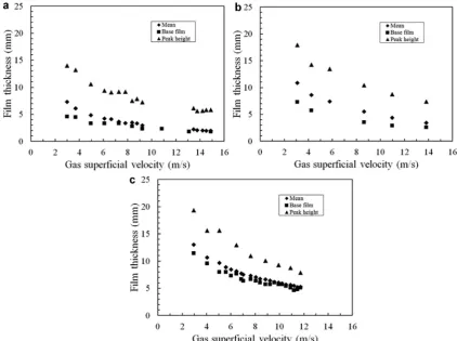
Values of the mean film thickness, that corresponding to the base film and of the average height of huge waves are plotted inFig. 18 for liquid superficial velocities of 0.11, 0.265 and 0.66 m/s. The base film thickness is seen to be slightly below the equivalent mean film thickness. Examination of the visualisations of the flow, such as those shown inFig. 8, indicted that the huge waves occupied only 20% of the film interface. This is confirmed by the work ofSekoguchi and Mori (1997), though it is noted that their data were from a smaller
diame-Fig. 19. Dimensionless mean film thickness plotted against dimensionless gas
veloc-ity. Closed symbols – present work. Liquid superficial velocity●0.11 m/s; 0.26 m/s;
0.41 m/s;0.66 m/s. Open symbols – Parsi et al. (2015). Liquid superficial velocity
◦0.3 m/s;0.46 m/s; ca% 0.61 m/s; a1% 0.76 m/s. Grey symbols –Hernandez Perez et al. (2010). Liquid superficial velocity=0.25 m/s.
ter pipe. From this it is not surprising that the mean film thickness is close to that of the base film.
The mean film thickness data, together with that from other sources, i.e., Hernandez Perez et al. (2010), Parsi et al; (2015a, 2015b), have been examined to determine parametric trends.Fig. 19 shows the mean film thickness data, non-dimensionalised by the pipe diameter, plotted against the inverse dimensionless gas velocity, 1/ug∗=[(
ρ
L-ρ
G)gD/ρ
Gu2Gs]. This shows that data from different pipe diameters are similar. In general, the dimensionless film thick-ness data depend onug∗to the power of∼ −0.67. A similar trend has [image:11.595.305.550.57.217.2] [image:11.595.80.503.410.725.2]Fig. 20. Product of dimensionless mean film thickness times the dimensionless gas velocity raised to the power of 0.67 plotted against liquid superficial velocity. Pipe di-ameters:Hernandez Perez et al. (2010)=67 mm;Parsi et al. (2015a, 2015b)=76 mm; present work=127 mm.
Fig. 21. Mean wave amplitude non-dimensionalised by mean film thickness.
been reported byKaji and Azzopardi (2010)for pipes of diameters be-tween 5 and 50 mm. If the data are replotted asug∗0.67<
δ
>/Dagainst the liquid superficial velocity, it can be seen inFig. 20that there is a small but significant relationship. The greatest scatter is seen for the data ofParsi et al. (2015a, 2015b) for their lowest liquid and highest gas superficial velocities. It is possible that these data are in annular flow.Wave amplitudes, the difference between peak heights and base film thicknesses made dimensionless by the mean film thicknesses, can also be extracted. The values obtained are illustrated inFig. 21; they show only a small effect of gas superficial velocity but a stronger effect of liquid superficial velocity.
[image:12.595.47.290.272.431.2] [image:12.595.316.558.299.481.2]The fraction of liquid in the film, which is travelling in waves as opposed to in the base film, has been determined using the method proposed bySawai et al. (2004). As shown inFig. 17, is not unreason-able to assume that the contribution of the base film in a plot of the Probability Density Function of dimensionless film thickness can be described by a Gaussian function. The difference between the over-all Probability Density Function and this Gaussian is the part of the liquid in the huge waves. The fraction of liquid in waves is plotted in Fig. 22for a liquid superficial velocity of 0.11 m/s and shows a grad-ual decrease as the gas velocity increases. Also shown is the nearest equivalent data from the work ofSawai et al. (2004). This was ob-tained in a smaller diameter pipe, 25.8 mm. The particular data set is chosen on the basis of the nearest liquid Reynolds number (
ρ
LuLsD/η
L) to the data from the present work. Both results show similar trends. The decrease in liquid fraction in the waves probablyFig. 22. Fraction of liquid in waves, i.e.,PWin the paper ofSawai et al. (2004)plotted against a dimensionless gas velocity, aȡ[ρ;Gu2
Gs/(ρL-ρG)gD]. Open symbols are data of Sawai et al. (2004)from a pipe diameter of 25.8 mm, closed symbols are from present work from a pipe diameter of 127 mm.
Fig. 23. Effect of gas and liquid superficial velocities on fraction of liquid in waves,i.e.,
PWin the paper ofSawai et al. (2004).
marks a transition towards annular flow whose Probability Density Function signature has no tail unlike churn flow. Data for a number of liquid superficial velocities are shown inFig. 23. For higher liq-uid superficial velocities the fraction of liqliq-uid in the waves takes a value of∼0.5 with a decrease becoming visible at the highest gas flow rate shown for the data from the liquid superficial velocity of 0.26 m/s. This indicates that the transition to annular flow occurs at higher gas velocities as the liquid velocity increases. This is contrary to the boundaries proposed byHewitt and Roberts (1969)and illus-trated in the modified version of their map shown inFig. 1and by Barnea (1986)who indicate a boundary which is almost independent of liquid flow rate. In contrast, the boundary proposed bySekoguchi and Mori (1997), based on the flow rates at which huge wave and disturbance wave frequencies are equal, indicates higher liquid flow rates and the gas flow rate increases. These types of plots show a way of discriminating between churn and annular flow.
Fig. 24. Single frame of Wire Mesh Sensor output showing distribution of the phases about the cross-section. Gas superficial velocity 3 m/s, liquid superficial velocity=
[image:13.595.59.258.58.258.2]0.265 m/s.
Fig. 25.Sequence frames of Wire Mesh Sensor output showing distribution of the
phases about the cross-section together with time trace of dimensionless film thick-ness focussing on crests of huge waves. Gas superficial velocity=3 m/s, liquid superfi-cial velocity=0.265 m/s.
clear from the figure that the film is not circumferentially uniform. There are large protrusions into the core at several positions around the pipe. These are probably parts of a huge wave. The part at the top is an example of the start of atomisation, i.e., the formation of a lig-ament which might be interpreted as a wisp. Also seen in the core of the pipe are a number of drops which appear in yellow as they do not occupy the whole of the particular pixel. A number of further examples of such views are shown inFig. 25where they are identi-fied with the positions of the (averaged) dimensionless film thickness time trace to which they correspond. Most of these frames are from the peaks of waves. A second sequence,Fig. 26, provides views from positions along two huge waves and the portion in between which contains a large wisp. These show the multidimensional complexity present. It is noted that though the Wire Mesh Sensor gives a great deal of information, it does not provide the fine detail that would be necessary for advanced mathematical modelling. For that an alterna-tive approach such as the Brightness Based Laser Induced Fluores-cence, employed byCherdantsev et al. (2014)would be required.
[image:13.595.306.550.282.448.2]Indirect evidence about the transport of liquid entrained as drops can be found in the wall shear stress,
τ
W, measurements ofZangana and Azzopardi (2012). They employed the same flow facility as theFig. 26. Sequence frames of Wire Mesh Sensor output showing distribution of the
phases about the cross-section together with time trace of dimensionless film thick-ness illustrating changes over two huge waves and a wisp. Gas superficial velocity=
3 m/s, liquid superficial velocity=0.265 m/s.
Fig. 27. Wall shear stress measured byZangana and Azzopardi (2012),♦, using a hot
film probe together with values,, calculated employing the film thickness obtained from the Wire Mesh Sensor with allowance for the entrained fraction shown. The cor-responding entrained fraction values are plotted as the solid line.
present work and used a carefully calibrated hot film probe and mon-itored temperature of the liquid at the wall either side of the hot film probe to determine the direction of flow. Examples of their results are shown inFig. 27together with values calculated from
τ
W=fF
ρ
Lu2F2 (5)
The friction factor, fF, was calculated using the stan-dard Blasius relationship using the Reynolds number (Re =
ρ
LuFDHF/η
L =ρ
LusLD/η
L), and uF is the mean velocity of the film – obtained from the liquid flow rate andDHFis the hydraulic diameter for the film which is equal to 4δ
(D−δ
)/Dandδ
is the mean film thickness determined above but allowing for the fact that some of the liquid was travelling as entrained drops andη
L is the liquid viscosity. Because of the poor agreement between the available methods for calculating the entrained fraction,Ef, and experimental data shown inFig. 4,Efwas calculated from the empirical equationEf= Ef0− A
(
uGs− uGsp)
2 (6) [image:13.595.38.279.304.469.2]Fig. 28. Velocities of huge waves calculated from time delay obtained from cross-correlation of time traces from two adjacent conductance probes.
shows the same trend as the available data plotted inFig. 4which was from a lower liquid flow rate. In spite of the difference in flow rates between the data inFigs. 4and27, the good agreement between mea-sured and calculated wall shear stress gives some confidence that the entrained fraction is as shown inFig. 27.
The velocity of the periodic structures has been calculated from the delay times obtained by cross-correlating the times series from two axially-separated conductance probes. The results are displayed inFig. 28together with the line showing the value that would be ex-pected for slug flow, 1.4um+ 0.35(gD). As expected, the values deter-mined from the experiments are all below the slug flow line. The de-viation appears to occur at higher gas superficial velocities for larger values of liquid superficial velocity. These results also show the max-ima and minmax-ima found in all other churn flow data as presented by Azzopardi (2006). If the data inFig. 28is examined further, it is seen that a great part of it lies in almost horizontal lines, indicating they this velocity is almost independent of gas flow rate. This is seen more clearly if they are plotted as the ratio of huge wave velocity to liq-uid superficial velocity against gas superficial velocity. The data still appear independent of gas flow but do not collapse on to one line indicating a more complex dependence on liquid flow rate.
Frequency characteristics of the times series can be obtained us-ing Power Spectrum analysis. Here, Power Spectrum Densities (PSD) have been obtained by using the Fourier transform of the auto covari-ance functions of the time series of cross-sectionally averaged void fraction. From the variation of PSD with frequency, the most proba-ble frequencies, the peak frequency, have been extracted. The results are presented in inFig. 29and show that frequency increases with increasing liquid superficial velocity and passes through a minimum with increasing gas superficial velocity.
For annular flow, a mechanistic model may be applied employing force balances on the wall film and the drop laden gas core. In this the fraction of liquid entrained as drops as well as the wall and interfacial shear stress need to be specified. This would enable film thicknesses to be calculated. Though there are reasonable methods to determine entrained fraction in annular flow, as shown inFig. 4, the same cannot be said in churn flow and so the approach cannot be implemented.
Occurrence and frequencies of wisps
[image:14.595.316.558.58.239.2]The conditions at which wisps occurred from all the published sources described above have been plotted on the modified He-witt and Roberts flow pattern map, i.e., a plot liquid Weber num-ber against gas Wenum-ber numnum-bers. These conditions are shown in Fig. 30together with the conditions at which wisps were identified in the present study. The plot illustrates that wisps occur over broad
Fig. 29.Effect of flow rate on frequency extracted from cross-sectionally averaged void
[image:14.595.317.557.275.445.2]fraction determined from the Wire Mesh Sensor.
Fig. 30. Flow pattern maps showing conditions at which Big wisps, small wisps and
no wisps occur.Big wisps;Small wisps;●No wisps. Other observations of wisps:
Hewitt and Roberts (1969);Sekoguchi and Mori (1997);●Hawkes et al. (2000);
♦Prasser et al. (2002);◦Omebere-Iyari et al. (2008);Hernandez Perez et al. (2010).
Fig. 31.Ratio of the frequencies of wisps to those of huge waves plotted against di-mensionless gas velocity. Open symbols – present work; closed symbols –Hernandez Perez et al. (2010).
can be associated with a particular huge wave. This is not surprising if the wisps are considered ligaments, part of the process of atomi-sation. These arise from instabilities at different points of the wave surface.
Conclusions
From the above, the following conclusions can be drawn:
• The flow in the 127 mm diameter pipe over range of gas superficial velocities of 3–15 m/s and liquid superficial velocities of 0.053– 0.66 m/s is in the churn flow pattern with its characteristic huge waves. It also shows wisps similar to those reported byHernandez Perez et al. (2010).
• The cross-sectional and time averaged void fraction for churn flow can be described by a drift flux type equation. For this flow pat-tern the distribution coefficient takes a value of∼1.0 as expected for flows with gas continuous core. The equivalent to the drift ve-locity is best described by the drift veve-locity for slug flow plus the mixture velocity at the transition to churn flow times the differ-ence in distribution coefficients for slug and churn flows. • Mean film thicknesses together with those for the base film and
the peaks of the waves have been extracted from the Wire Mesh Sensor output. These data together with that from published pa-pers show a strong trend with gas flow rate and a weaker one with liquid flow rate. There seems to be little effect of pipe diam-eter. However, it is clear that the waves are not circumferentially uniform.
• Wisps of different sizes have been observed over most the range of flow rates studied with the exception of the higher gas ve-locities. This is in agreement with many of the observations of wisps reported in the literature. The frequency of occurrence of wisps decreases with increasing gas superficial velocity. Their values are usually, but not always, lower than the correspond-ing frequency of huge waves. There is clear evidence that wisps arise from huge waves and are part of an incomplete atomisation process.
Acknowledgements
SS was supported by an EPSRC studentship as part of Grant number EP/F016050/1. This research study has been undertaken within the Joint Project on Transient Multiphase Flows and Flow As-surance. The Authors wish to acknowledge the contributions made
to this project by the UK Engineering and Physical Sciences Research Council (EPSRC) and the following: Advantica; BP Exploration Oper-ating Co. Ltd.; CD-adapco; Chevron; ConocoPhillips; ENI; ExxonMo-bil; FEESA; IFP; Institutt for Energiteknikk; Norsk Hydro; PDVSA (IN-TERVEP); Petrobras; PETRONAS; ScandpowerPT; Shell; SINTEF; Sta-toil and TOTAL. This provided support for GPvdM. The Authors wish to express their gratitude for this support.
References
Ahmad, M., Peng, J.D., Hale, C.P., Walker, S., Hewitt, G.F., 2010. Droplet entrainment in churn flow. In: Proceedings of International Conference on Multiphase Flow. (ICMF-2010), May 30 - June 4 2010. Tampa, Florida.
Azzopardi, B.J., 1983. Mechanisms of Entrainment in Annular Two-phase Flow. UKAEA Report AERE-R 11068.
Azzopardi, B.J., 2006. Gas–Liquid Flows. Begell House, New York.
Azzopardi, B.J., Abdulkareem, L., Zhao, D., Thiele, S., Da Silva, M., Beyer, M., 2010. Com-parison between electrical capacitance tomography and wire mesh sensor output for air/silicone oil flow in a vertical pipe. Ind. Eng. Chem. Res. 49, 8805–8811. Barbosa, J.R., Govan, A.H., Hewitt, G.F., 2001. Visualisation and modelling studies of
churn flow in a vertical pipe. Int. J. Multiph. Flow 27, 2105–2127.
Barbosa, J.R., Hewitt, G.F., König, G., Richardson, S.M., 2002. Liquid entrainment, droplet concentration and pressure gradient at the onset of annular flow in a vertical pipe. Int. J. Multiph. Flow 28, 943–961.
Barnea, D., 1986. Transition from annular flow and from dispersed bubble flow - unified models for the whole range of pipe inclinations. Int. J. Multiph. Flow 12, 733–744. Bennett, A.W., Hewitt, G.F., Kearsey, H.A., Keeys, R.K., Lacey, P.M., 1965. Flow
visualisa-tion studies of boiling at high pressure. Proc. Inst. Mech. Eng. 180, 1–11. Bhagwat, S.M., Ghajar, A.J., 2014. A flow pattern independent drift flux model based
void fraction correlation for a wide range of gas–liquid two phase flow. Int. J. Mul-tiph. Flow 59, 186–205.
Brauner, N., Barnea, D., 1986. Slug/churn transition in upward gas–liquid flow. Chem. Eng. Sci. 40, 159–163.
Brauner, N., Ullmann, A., 2004. Modelling of gas entrainment from Taylor bubbles. Part A: slug flow. Int. J. Multiph. Flow 30, 239–272.
Cheng, H., Hills, J.H., Azzopardi, B.J., 1998. A study of the bubble-to-slug transition in vertical gas-liquid flow in columns of different diameters. Int. J Multiph. Flow 24, 431–452.
Cheng, H., Hills, J.H., Azzopardi, B.J., 2002. Effects of initial bubble size on flow pattern transition in a 28.9 mm diameter column. Int. J Multiph. Flow 28, 1047–1062. Cherdantsev, A.V., Hann, D.B., Azzopardi, B.J., 2014. Study of gas-sheared liquid film
in horizontal rectangular duct using high-speed LIF technique: three-dimensional wavy structure and its relation to liquid entrainment. Int. J. Multiph. Flow 67, 52– 64.
Costigan, G., Whalley, P.B., 1997. Slug flow regime identification from dynamic void fraction measurements in vertical air–water flows. Int. J. Multiph. Flow 23, 263– 282.
Da Riva, E., Del Col, D., 2009. Numerical simulation of churn flow in a vertical pipe. Chem. Eng. Sci. 64, 3753–3765.
de Cachard, F., Delhaye, J.M., 1996. A slug-churn model for small-diameter airlift pumps. Int. J. Multiph. Flow 22, 627–649.
Dukler, A.E., Taitel, Y., 1977. Flow Regime Tensition for Verticl Upward Flow: A Prelimi-nary Approach Through Physical Modelling. Prog. Report no. 1, NUREG-0162.
Fernandes, R.C., Semiat, R., Dukler, A.E., 1983. Hydrodynamic model for gas–liquid slug flow in vertical tubes. AIChE J. 29, 981–989.
Govier, G.W., Short, L.W., 1958. The upward vertical flow of air–water mixtures – I. Effect of air and water flow rates on flow pattern, hold-up and pressure drop. Can. J. Chem. E. 36, 195–202.
Guet, S., Ooms, G., Oliemans, R.V.A., Mudde, R.F., 2004. Bubble size effect on low liquid input drift–flux parameters. Chem. Eng. Sci. 59, 3315–3329.
Guet, S., Decarre, S., Henriota, V., Liné, A., 2006. Void fraction in vertical gas–liquid slug flow: influence of liquid slug content. Chem. Eng. Sci. 61, 7336–7350.
Hawkes, N.J., Lawrence, C.J., Hewitt, G.F., 2000. Studies of wispy-annular flow using transient pressure gradient and optical measurements. Int. J. Multiph. Flow 26, 1562–1592.
Hawkes, N.J., Lawrence, C.J., Hewitt, G.F., 2001. Prediction of the transition from annular to wispy-annular flow using linear stability analysis of the gas-droplet core. Chem. Eng. Sci. 56, 1925–1932.
Hernandez Perez, V., Azzopardi, B.J., Kaji, R., Da Silva, M.J., Beyer, M., Hampel, U., 2010. Wisp-like structures in vertical gas–liquid pipe flow revealed by wire mesh sensor studies. Int.J. Multiph. Flow 36, 908–915.
Hewakandamby, B.N., Kanu, A.U., Azzopardi, B.J., Kouba, G., 2014. Parametric study of churn flow in large diameter pipes. In: Proceedings of Fourth ASME Joint US– European Fluids Engineering Summer Meeting. FEDSM2014, August 3–7, 2014. Chicago, Illinois.
Hewitt, G.F., Roberts, D.N., 1969. Studies of Two-Phase Patterns by Simultaneous X-ray and Flash Photography. UKAEA Report AERE M2159.
Hewitt, G.F., Martin, C.J., Wilkes, N.S., 1985. Experiment and modelling studies of an-nular flow in the region between flow reversal and the pressure drop minimum. Phys.-Chem. Hydrodyn. 6, 69–86.
Hewitt, G.F., Govan, A.H., 1990. Phenomenological modelling of non-equilibrium flow with phase change. Int. J. Heat Mass Transf. 32, 229–242.
Hinze, J.O., 1955. Fundamentals of the hydrodynamic mechanism of splitting of disper-sion processes. AIChE J. 1, 289–295.
Jones, O., Zuber, N., 1975. The interrelation between void fraction fluctuations and flow patterns in two-phase flow. Int. J. Multiph. Flow 2, 273–306.
Jacowitz, L.A., Brodkey, R.S., 1964. An analysis of geometry and pressure drop for the horizontal, annular, two-phase flow of water and air in the entrance region of a pipe. Chem. Eng. Sci. 19, 261–274.
Jayanti, S., Hewitt, G.F., 1992. Prediction of the slug-to-churn transition in vertical two-phase flow. Int. J. Multiph. Flow 18, 847–860.
Kaji, R., 2008. Characteristics of Two-phase Flow Structures and Transitions in Vertical Upflow (Ph.D. thesis). University of Nottingham.
Kaji, R., Hills, J.H., Azzopardi, B.J., 2009. Extracting information from time series data in vertical up flow. Multiph. Sci. Technol. 21, 1–12.
Kaji, R., Azzopardi, B.J., Lucas, D., 2009. Investigation of flow development of co-current gas–liquid vertical slug flow. Int. J. Multiph. Flow 35, 335–348.
Kaji, R., Azzopardi, B.J., 2010. The effect of pipe diameter on the structure of gas/liquid flow in vertical pipes. Int. J. Multiph. Flow 36, 303–313.
McQuillan, K.W., Whalley, P.B., 1985. Flow patterns in vertical two-phase flow. Int. J. Multiph. Flow 11, 161–176.
Mishima, K., Ishii, M., 1984. Flow regime transition criteria for two-phase flow in ver-tical tubes. Int. J. Heat Mass Transf. 27, 723–734.
Nicklin, D.J., Davidson, J.F., 1962. The onset of instability in two-phase slug flow. In: Proceedings of Mechanical Engineering Symposium on Two-Phase Flow. London Paper 5.
Omebere-Iyari, N.K., 2006. The Effect of Pipe Diameter and Pressure in Vertical Two-phase Flow (Ph.D. thesis), University of Nottingham.
Omebere-Iyari, N.K., Azzopardi, B.J., 2007. A study of flow patterns for gas/liquid flows in small diameter tubes. Chem. Eng. Res. Des. 85, 180–192.
Omebere-Iyari, N.K., Azzopardi, B.J., Lucas, D., Beyer, M., Prasser, H.M., 2008. The char-acteristics of gas/liquid flow in large risers at high pressures. Int. J. Multiph. Flow 34, 461–476.
Parsi, M., Vieira, R.E., Torres, C.F., Kesana, N.R., McLaury, B.S., Shirazi, S.A., Schleicher, E., Hampel, U., 2015a. Experimental investigation of interfacial structures within churn flow using a dual wire-mesh sensor. Int. J. Multiph. Flow 73, 155–170. Parsi, M., Vieira, R.E., Torres, C.F., Kesana, N.R., McLaury, B.S., Shirazi, S.A., Schleicher, E.,
Hampel, U., 2015b. On the effect of liquid viscosity on interfacial structures within churn flow: experimental study using wire mesh sensor. Chem. Eng. Sci. 130, 221– 238.
Pinto, A.M.F.R., Coelho Pinheiros, M.N., Campos, J.B.L.M., 1998. Coalescence of two gas slugs rising in a co-current flowing liquid in vertical tubes. Chem. Eng. Sci. 53, 2973–2983.
Prasser, H.-M., Zschau, J., Peters, D., Pietzsch, G., Taubert, W., Trepte, M., 2002. Fast wire-mesh sensors for gas-liquid flows - visualisation with up to 10,000 frames per sec-ond. In: Proceedings of International Congress on Advanced Nuclear Power Plants (ICAPP), June 9–13, 2002. Hollywood Florida, USA Proc. CD-ROM, paper #1055. Prasser, H.-M., Böttger, A., Zschau, J., 1998. A new electrode-mesh tomograph for
gas-liquid flows. Flow Meas. Instrum. 9, 111–119.
Rodriguez, D.J., Shedd, T.A., 2004. Entrainement of gas in the liquid film of horizontal, annular, two-phase flow. Int J. Multiph. Flow 30, 565–583.
Sawai, T., Kaji, M., Kasugai, T., Nakashima, H., Mori, T., 2004. Gas–liquid interfacial struc-ture and pressure drop characteristics of churn flow. Exp. Therm. Fluid Sci. 28, 597– 606.
Sekoguchi, K., Mori, K., 1997. New development of experimental study on interfacial structure in gas-liquid two-phase flow. Exp. Heat Transf. Fluid Mech. Thermodyn. Sharaf, S., Da Silva, M., Hampel, U., Zippe, C., Beyer, M., Azzopardi, B.J., 2011. Comparison
between wire mesh sensor and gamma densitometry void measurements in two-phase flows. Meas. Sci. Technol. 22 (104019).
Sylvester, N.D., 1987. A mechanistic model for two-phase vertical slug flow in pipes. J. Energy Res. Technol. 109, 206–213.
Szalinski, L., Abdulkareem, L.A., Da Silva, M.J., Thiele, S., Beyer, M., Lucas, D., Hernandez-Perez, V., Hampel, U., Azzopardi, B.J., 2010. Comparative study of gas–oil and gas– water two-phase flow in a vertical pipe. Chem. Eng. Sci. 65, 3836–3848. Taitel, Y., Barnea, D., Dukler, A.E., 1980. Modelling flow pattern transitions for steady
upward gas–liquid flow in vertical tubes. AICh E J. 26, 345–354.
van der Meulen, G.P., 2012. Churn-Annular Gas–Liquid Flows in Large Diameter Vertical Pipes (Ph.D. thesis), University of Nottingham
Verbeek, P.H.J., Miesen, R., Schellenkens, C.J., 1992. Liquid entrainment in annular dis-persed upflow. In: Proceedings of the 8th Annual European Conference on Liquid Atomisation and Spray Systems. 30 September–2 October. Amsterdam.
Verbeek, P.R.J., Miesen, R., Schellenkens, C.J., 1993. Liquid entrainment in annular dis-persed upflow. In: Proceedings of European Two-Phase Flow Group Meeting. 7–10 June. Hannover (cited by Barbosa et al. (2002)).
Viana, F., Pardo, R., Yanez, R., Trallero, J.L., Joseph, D.D., 2003. Universal correlation for the rise velocity of long gas bubbles in round pipes. J. Fluid Mech. 494, 379–398. Waltrich, P.J., Falcone, G., Barbosa Jr., J.R., 2013. Axial development of annular, churn
and slug flows in a long vertical tube. Int. J. Multiph. Flow 57, 38–48.
Wallis, G.B., Steen, D.A., Brenner, S.N., Turner, J.M., 1963. Joint US-Euratom Research and Development Programme, Quarterly Progress Report, April 1963. Dartmouth College Report NYO-10488, USA.
Wang, K., Bai, B., Cui, J., Ma, W., 2012. A physical model for huge wave movement in gas–liquid churn flow. Chem. Eng. Sci. 79, 19–28.
Wang, K., Bai, B., Ma, W., 2013a. Huge wave and drop entrainment mechanism in gas-liquid churn flow. Chem. Eng. Sci. 104, 638–646.
Wang, K., Bai, B., Ma, W., 2013b. A model for droplet entrainment in churn flow. Chem. Eng. Sci. 104, 1045–1055.
Watson, M.J., Hewitt, G.F., 1999. Pressure effects on the slug to churn transition. Int. J. Multiph. Flow 25, 1225–1241.
Westende, J.M.C., van ’t Kemp, H.K., Belt, R.J., Portela, L.M., Mudde, R.F., Oliemans, R.V.A., 2007. On the role of droplets in cocurrent annular and churn-annular pipe flow. Int. J. Mulitph. Flow 33, 595–615.
Zangana, M.H.S., Azzopardi, B.J., 2012. Liquid film properties of gas–liquid flow in large diameter vertical pipe. WIT Trans. Eng. Sci. 81, 231–242.
Zhang, Z, Bieberle, M, Barthel, F., Szalinski, L., Hampel, U., 2013. Investigation of upward cocurrent gas–liquid pipe flow using ultrafast X-ray tomography and wire-mesh sensor. Flow Meas. Instrum 32, 111–118.