A robust similarity measure for volumetric image registration with outliers

(1)

006 007 008 009 010 011 012 013 014 015 016 017 018 019 020 021 022 023 024 025 026 027 028 029 030 031 032 033 034 035 036 037 038 039 040 041 042 043 044 045 046 047 048 049 050 051 052 053 054 055 056 057 058 059 060 061 062 063 064 065 066

072 073 074 075 076 077 078 079 080 081 082 083 084 085 086 087 088 089 090 091 092 093 094 095 096 097 098 099 100 101 102 103 104 105 106 107 108 109 110 111 112 113 114 115 116 117 118 119 120 121 122 123 124 125 126 127 128 129 130 131 132

Journal: IMAVIS

Article Number: 03507

Please e-mail your responses and any corrections to:

E-mail:

Corrections.ESCH@elsevier.spitech.com

Dear Author,

Please check your proof carefully and mark all corrections at the appropriate place in the proof (e.g., by using on-screen annotation

in the PDF file) or compile them in a separate list. Note: if you opt to annotate the file with software other than Adobe Reader then

please also highlight the appropriate place in the PDF file. To ensure fast publication of your paper please return your corrections

within 48 hours.

For correction or revision of any artwork, please consult

http://www/elsevier.com/artworkinstructions

.

We were unable to process your file(s) fully electronically and have proceeded by

Scanning (parts of) your

article

Rekeying (parts of) your

article

Scanning the

artwork

Any queries or remarks that have arisen during the processing of your manuscript are listed below and highlighted by flags in the

proof. Click on the ‘Q’ link to go to the location in the proof.

Location in article

Query / Remark:

click on the Q link to go

Please insert your reply or correction at the corresponding line in the proof

Q1

Your article is registered as a regular item and is being processed for inclusion in a regular issue of

the journal. If this is NOT correct and your article belongs to a Special Issue/Collection please contact

michael.evans@elsevier.com immediately prior to returning your corrections.

Q2

The author names have been tagged as given names and surnames (surnames are highlighted in teal

color). Please confirm if they have been identified correctly.

Q3

The term "experimental section" has been changed to "Experiments section" so as to match and link

it with the section heading "Experiments". Please check if this change is appropriate, and correct if

necessary.

Q4

Please provide the grant numbers for "Qualcomm", "Imperial College London" and "Seventh Framework

Programme".

Q5

One sponsor name "7th Framework Programme" has been edited to a standard format "Seventh

Frame-work Programme" that enables better searching and identification of your article. Please check and

correct if necessary.

Please check this box or indicate your approval if

you have no corrections to make to the PDF file.

Thank you for your assistance.

(2)

133

134

135

136

137

138

139

140

141

142

143

144

145

146

147

148

149

150

151

152

153

154

155

156

157

158

159

160

161

162

163

164

165

166

167

168

169

170

171

172

173

174

175

176

177

178

179

180

181

182

183

184

185

186

187

188

189

190

191

192

193

194

195

196

197

198

199

200

201

202

203

204

205

206

207

208

209

210

211

212

213

214

215

216

217

218

219

220

221

222

223

224

225

226

227

228

229

230

231

232

233

234

235

236

237

238

239

240

241

242

243

244

245

246

247

248

249

250

251

252

253

254

255

256

257

258

259

260

261

262

263

264 Contents lists available atScienceDirect

Image and Vision Computing

j o u r n a l h o m e p a g e : w w w . e l s e v i e r . c o m / l o c a t e / i m a v i s

Highlights

Image and Vision Computing xxx (2016) xxx–xxx

A robust similarity measure for volumetric image registration with outliers

Patrick Snapea,_*_{, Stefan Pszczolkowski}c_{, Stefanos Zafeiriou}a_{, Georgios Tzimiropoulos}b_,

Christian Lediga_{, Daniel Rueckert}a

a_{Imperial College London, Department of Computing, London SW7 2AZ, UK} b_{University of Nottingham, School of Computer Science, Nottingham NG8 1BB, UK} c_{University of Nottingham, School of Medicine, Nottingham NG7 2UH, UK}

• Investigation of robust alignment methods for volumetric medical images

• Proposal of two novel similarity measures based on the cosine of normalised 3D volumetric gradients

• The measures are shown to be robust to occlusions and bias ﬁeld corruption.

• The ﬁrst review of robust 3D Lucas–Kanade methods for aﬃne image alignment

• The proposed methods show good performance for non-rigid alignment.

http://dx.doi.org/10.1016/j.imavis.2016.05.006

(3)

UNCORRECTED

PR

OOF

265

266

267

268

269

270

271

272

273

274

275

276

277

278

279

280

281

282

283

284

285

286

287

288

289

290

291

292

293

294

295

296

297

298

299

300

301

302

303

304

305

306

307

308

309

310

311

312

313

314

315

316

317

318

319

320

321

322

323

324

325

326

327

328

329

330

331

332

333

334

335

336

337

338

339

340

341

342

343

344

345

346

347

348

349

350

351

352

353

354

355

356

357

358

359

360

361

362

363

364

365

366

367

368

369

370

371

372

373

374

375

376

377

378

379

380

381

382

383

384

385

386

387

388

389

390

391

392

393

394

395

396 Contents lists available atScienceDirect

Image and Vision Computing

j o u r n a l h o m e p a g e : w w w . e l s e v i e r . c o m / l o c a t e / i m a v i s

A robust similarity measure for volumetric image registration

with outliers

夽

Q1

Q2

Patrick

Snape

a,

*

,

Stefan

Pszczolkowski

c

,

Stefanos

Zafeiriou

a

,

Georgios

Tzimiropoulos

b

,

Christian

Ledig

a

_,

_Daniel

_Rueckert

a

a_{Imperial College London, Department of Computing, London SW7 2AZ, UK} b_{University of Nottingham, School of Computer Science, Nottingham NG8 1BB, UK} c_{University of Nottingham, School of Medicine, Nottingham NG7 2UH, UK}

A R T I C L E I N F O

Article history:

Received 9 February 2015

Received in revised form 30 April 2016 Accepted 5 May 2016

Available online xxxx

Keywords: Image registration Lucas–Kanade Normalised gradient Free-form deformation

A B S T R A C T

Image registration under challenging realistic conditions is a very important area of research. In this paper, we focus on algorithms that seek to densely align two volumetric images according to a global similarity measure. Despite intensive research in this area, there is still a need for similarity measures that are robust to outliers common to many different types of images. For example, medical image data is often corrupted by intensity inhomogeneities and may contain outliers in the form of pathologies. In this paper we propose a global similarity measure that is robust to both intensity inhomogeneities and outliers without requiring prior knowledge of the type of outliers. We combine the normalised gradients of images with the cosine function and show that it is theoretically robust against a very general class of outliers. Experimentally, we verify the robustness of our measures within two distinct algorithms. Firstly, we embed our similarity measures within a proof-of-concept extension of the Lucas–Kanade algorithm for volumetric data. Finally, we embed our measures within a popular non-rigid alignment framework based on free-form deformations and show it to be robust against both simulated tumours and intensity inhomogeneities.

1. Introduction

Image registration is an important procedure in many areas of computer vision for both 2D and volumetric 3D images. Given its relevance, there is a large body of prior work concentrating on methodologies for performing accurate registration. In this paper, we are most interested in techniques that attempt to densely align two images according to a global similarity measure. Many global simi-larity measures have been proposed, yet only a few focus on being robust to the presence of outliers and systematic errors. We consider a similarity measure to be robust if it is not biased by the presence of noise and/or occlusions within the image to be registered. Gener-ally, if a similarity measure is biased by noise or occlusions, this will manifest as a failure to accurately register the images.

夽This paper has been recommended for acceptance by Ioannis A. Kakadiaris, PhD. *Corresponding author.

E-mail addresses:p.snape@imperial.ac.uk(P. Snape),

stefan.pszczolkowskiparraguez@nottingham.ac.uk(S. Pszczolkowski),

s.zafeiriou@imperial.ac.uk(S. Zafeiriou),yorgos.tzimiropoulos@nottingham.ac.uk

(G. Tzimiropoulos),christian.ledig@imperial.ac.uk(C. Ledig),

d.rueckert@imperial.ac.uk(D. Rueckert).

In the case of 2D images, systematic errors and outliers are com-mon in the form of illumination variance and occlusions, which naturally occur in so called “in-the-wild” images. Although 2D image alignment is a broad field, much of the existing work focuses on aug-menting existing efficient algorithms with improved robust proper-ties. For example, one of the first algorithms to describe a 2D image alignment approach was the Lucas–Kanade (LK) algorithm[1]. The LK algorithm concentrates on recovering a warp that best maximises a similarity measure between two images. Numerous extensions to the LK algorithm have been proposed[2,3,4]and most are based on

2 norm minimisation[3,5,6,7]. Most notably, the inverse compo-sitional framework proposed by Baker and Matthews[5]provides a computationally eﬃcient framework for solving the least squares problem.

For volumetric, or 3D images, outliers can occur in the form of pathologies, and systematic errors are commonly seen as inten-sity inhomogeneities caused by image acquisition artefacts such as bias ﬁelds[8]. Several methods have been proposed for registra-tion of medical images with mismatches, focusing on robustness[9], tumour models [10]or Bayesian models[11]. However, previous methods[12]all require prior knowledge of what constitutes a mis-match in order to detect and ignore them. Additionally, a number of

http://dx.doi.org/10.1016/j.imavis.2016.05.006

(4)

UNCORRECTED

PR

OOF

397

398

399

400

401

402

403

404

405

406

407

408

409

410

411

412

413

414

415

416

417

418

419

420

421

422

423

424

425

426

427

428

429

430

431

432

433

434

435

436

437

438

439

440

441

442

443

444

445

446

447

448

449

450

451

452

453

454

455

456

457

458

459

460

461

462

463

464

465

466

467

468

469

470

471

472

473

474

475

476

477

478

479

480

481

482

483

484

485

486

487

488

489

490

491

492

493

494

495

496

497

498

499

500

501

502

503

504

505

506

507

508

509

510

511

512

513

514

515

516

517

518

519

520

521

522

523

524

525

526

527

528 methods based on mutual information have been proposed to reduce

the effect of intensity inhomogeneities in the registration[13,14,15]. To the best of our knowledge, no existing similarity measure pro-vides robustness against both outliers and intensity inhomogeneities for registration of 3D imageswithout prior knowledge of the type of dissimilarity. However, the 2D similarity measure recently proposed inRef.[16], has been shown to be robust against both general occlu-sions and illumination variance. This measure is formulated as the cosine of normalised gradient orientations and is simple and eﬃ-cient to compute. For 3D images, we seek to provide a similarity measure that can utilise the robust properties of the cosine func-tion. This requires calculating a similarity between the two images being aligned that can be represented as an angle. In this work, we provide two separate methodologies of measuring angular similarity between 3D images.

We clarify that when we state 3D images, we are referring to vol-umetric data where it is valid to compute gradients along all 3 of the principle axes. This may be in contrast to other usages of the term “3D” when referring to data sources such as range images or mesh data. In this case, we would refer to these data sources as 2.5D data, as the computation of the gradient for the depth axis is non-trivial. In fact, as mentioned by Baker et al.[17], the inverse compositional algorithm is no longer valid when extended to 2.5D data due to the representation of the data as a surface. Therefore, given that the treatment of 2.5D data is totally different from the 3D volumetric images that we use here, we do not further consider it.

It is important to note that there is a large amount of exist-ing work on usexist-ing gradient information for image registration on volumetric data. The concept of normalised image gradients was introduced to the ﬁeld of medical image registration by Pluim et al.[18]. InRef.[18], normalised mutual information (NMI)[19]is weighted voxelwise by the normalised image gradients in order to incorporate spatial information. After this initial work, the ﬁrst sim-ilarity based solely on normalised gradients was proposed by Haber and Modersitzki[20]. This similarity measure is based on thesquared cosineof the normalised gradients and is equivalent to minimising thesquared inner product. In contrast, our proposal is to use thecosine of the normalised gradient orientations and is equivalent to minimis-ing theinner product. This seemingly small difference, the squaring of the cosine, causes outliers to bias the similarity measure and thus affects the robustness. Despite these properties of the squared cosine measure, it has been successfully utilised in the literature[21,22,23]

for registering images that do not contain outliers.

Preliminary work on the cosine of orientations has been shown in our previous work[24,25]. InRef.[24], we gave preliminary results that show that the cosine of normalised gradient orientations repre-sents a robust similarity measure in the presence of both occlusions and intensity inhomogeneities. We extend this work in two major areas:

Firstly, we note that that there are two separate angular measures that can be deﬁned in order to compute the cosine of normalised gra-dient orientations between two images. These orientations are based on the spherical coordinates of the gradients and the inner prod-uct between the gradients. As a proof of concept, we directly extend the methodology ofRef.[16]to provide evidence that our similar-ity measures are robust to occlusions and intenssimilar-ity inhomogeneities. Although the extension of LK-type algorithms to 3D is simple and was proposed inRef.[17], no previous investigation has been done on how similarity measures perform when extended to 3D. Since no previous work has investigated the use of 3D Lucas–Kanade for robust registration, we chose to extend existing robust 2D meth-ods into 3D. These extended state-of-the-art 2D methmeth-ods are then compared against using a synthetic dataset.

Secondly, in order to show that our similarity measures compete with state-of-the-art techniques, we embed them within a widely and successfully used non-rigid registration framework based on

free-form deformations (FFD)[26]. This FFD registration framework differs from our LK example as it is a local deformation model and thus contains many thousands of parameters. This large parame-ter space makes Gauss–Newton optimisation infeasible due to the memory requirements of inverting the Hessian matrix. For this rea-son, registration techniques that focus on local deformations are generally solved using gradient descent algorithms that incorpo-rate line searches[26]. We compare against the NMI measure[19], DRAMMS[27]and the cosine squared measure [20]and conﬁrm the robustness of the proposed similarity measures on simulated pathological data from a tumour database.Secondly, we provide more extensive evaluation into the robust properties of the cosine of normalised gradient orientations when applied to volumetric data.

The remainder of the paper is organised as follows. InSection 2

we discuss relevant related works and consider the advantages of our proposed measures. InSection 3we give a thorough explanation of the theory behind our work and empirically verify its robustness on our chosen data. InSection 4we describe the application of our sim-ilarity measure within the Lucas–Kanade algorithm and inSection 5

we show its application within the non-rigid framework of Rueck-ert et al.[26]. Experimental results within both rigid and non-rigid alignment are given inSection 6. Finally, we draw conclusions in

Section 7.

2. Related work

In this paper we are most interested in similarity measures that have been proposed for parametric image alignment. This is primarily due to the fact that parametric image alignment meth-ods are often very computationally eﬃcient. In particular, we are interested in approaches that show robustness to both intensity inhomogeneities and occlusions.

Within 2D image registration there has been a large body of work that focuses on illumination invariance. Within the most popular parametric image alignment framework, the Lucas–Kanade algorithm (LK), one of the the earliest attempts was by Hager and Belhumeur[28]. InRef.[28], the authors incorporate a linear appear-ance basis that models illumination variappear-ance and excelled in the area of object tracking. However, this requires prior knowledge of the type of object under consideration so that the appearance basis can be precomputed. There is a large amount of existing literature about incorporating prior knowledge via linear bases within the LK algorithm. However, we do not consider them here, as we are most interested in modelling unseen structured variation via robust simi-larity measures and thus prior knowledge is generally not available.

Within the LK framework, a number of robust measures have been proposed. Black and Jepson[29]proposed incorporating robust statistics into the LK framework and showed their effectiveness in the presence of illumination variance. Dowson and Bowden[3]

incorporated the mutual information (MI) measure within the LK framework and found it to be superior to an SSD based measure for illumination variance. However, using mutual information as a sim-ilarity measure requires updating the Jacobian and Hessian matrices at each iteration. For this reason, the MI measure is unable to make use of more computationally efficient LK algorithms such as the inverse compositional (IC) method proposed inRef.[5]. Although the authors do give an ad hoc solution that involves fixing the val-ues of the Jacobian and Hessian matrices, it is still a more complex implementation than the original inverse compositional algorithm. Evangelidis and Psarakis[6]provide a correlation measure between images and a computational framework that is invariant to illumina-tion differences. This is a great strength of the algorithm, however, the correlation measure is still grossly affected by outliers. Lucey et al.[4]propose a method of weighting the LK fitting with a large bank of filters in a computationally efficient manner. This is a very

(5)

UNCORRECTED

PR

OOF

529

530

531

532

533

534

535

536

537

538

539

540

541

542

543

544

545

546

547

548

549

550

551

552

553

554

555

556

557

558

559

560

561

562

563

564

565

566

567

568

569

570

571

572

573

574

575

576

577

578

579

580

581

582

583

584

585

586

587

588

589

590

591

592

593

594

595

596

597

598

599

600

601

602

603

604

605

606

607

608

609

610

611

612

613

614

615

616

617

618

619

620

621

622

623

624

625

626

627

628

629

630

631

632

633

634

635

636

637

638

639

640

641

642

643

644

645

646

647

648

649

650

651

652

653

654

655

656

657

658

659

660

1 (1, , )

Z

X

[image:5.595.67.266.58.246.2]

Y

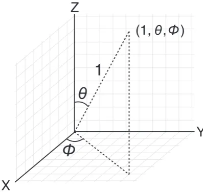
Fig. 1.An illustration of the spherical coordinate system as described in this paper.

effective technique and is largely illumination invariant, however, it gives little beneﬁt when presented with occlusions.

For 3D images, robust registration is a very active area of research. The most commonly used techniques for multi-modal registration are based on mutual information (MI)[30]. These techniques are highly effective at registration of objects with inherent structure such as anatomy but are very sensitive to global corruption such as intensity inhomogeneities. To overcome this, gradient information is often utilised and in particular was incorporated into a MI frame-work by Pluim et al.[18]. In particular, gradient information helps capture the local structure within an image which is not described by general MI-based registration techniques. Gradient information has also been successfully used in a number of other works[31,32,33]. However, these works focus on capturing local structure and not on robustness to artefacts such as pathologies caused by tumours. The most related work is that of Haber and Modersitzki[20], which pro-poses a similarity measure based on the square of the cosine (inner product squared). We conduct a thorough comparison with this technique and show that it is biased by the presence of occlusions.

Finally, the work of Tzimiropoulos et al.[16]introduced the ﬁrst similarity measure based on the cosine of normalised gradients. We would stress that although our work is inspired byRef.[16], the calculation of the orientations for our proposed similarities is very different. In particular, it is important to note that calculating an ori-entation in 3D is more complex than the 2D case due to the extra degree of freedom. In this work, we give a detailed explanation of how to calculate these orientations in 3D and how to optimise them for use in image registration.

3. Cosine of normalised gradients

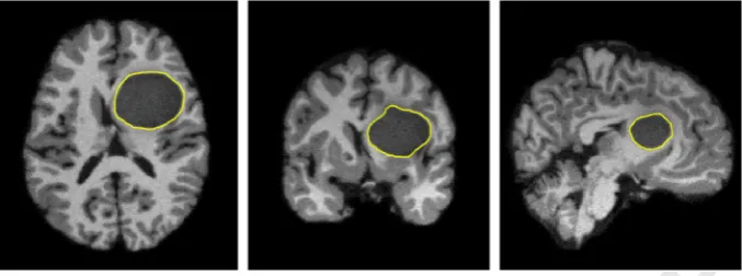
In this section, we describe the concept of the cosine of nor-malised gradients and specify how they represent a robust measure of similarity. In this work, we consider a similarity measure to be robust if it suppresses the contribution of comparisons between image areas that are unrelated. More speciﬁcally, we seek a measure that, when given two images that are visually dissimilar, will cal-culate zero correlation between them. For example, considerFig. 3

which shows cross sections of a brain containing a tumour. When registering this corrupted image with an image of a healthy brain, the ideal registration would not be biased by the presence of the tumour, as it does not share relevant anatomical structures with the healthy brain. To this end, Tzimiropoulos et al.[16,34]proposed the cosine of orientation differences between two images, which we describe in detail below.

3.1. Cosine similarity in 2D

Assumingthatwe are given two 2D images, denoted asIii∈ {1, 2},

we deﬁneGi,x =Fx∗Ii andGi,y=Fy∗Iias the gradients obtained

by convolvingIiwith differentiation approximation ﬁltersFxandFy

respectively. We denote the lexicographical vectorisation ofGi,xas

g_i_,_xand define an indexkinto the vector,g_i_,_x(k). We define an iden-tical vector forGi,yasgi,y. We also definegi(k) as the vector formed

by concatenating thexandygradients together. Trivially, we can deﬁne the normalised gradient as g˜i(k) = g_g_ii(₍k_k)₎ where gi(k)=

gi,x(k)2+gi,y(k)2. We also deﬁne similar vectors for thex andy

components separately, withg˜i,x being thexcomponents

concate-nated in lexicographical ordering andg˜i,ybeing theycomponents.

Finally, g˜i is the vector of concatenated normalised gradients for

imageIi.

Given the normalised gradients, it is simple to parametrise them within a polar coordinate system with radius ri(k) = ˜gi(k)= 1,

orientation0i(k) = arctan

˜

gi,y(k)

˜

gi,x(k) and pole at the origin. Given

ori-entations from two dissimilar images, it is reasonable to assume that difference between the orientations, D0(k) = 01(k)−02(k), can take any angle between [0, 2p). Intuitively, this implies that selecting two pixels from dissimilar images is unlikely to yield any correlation between the images. InRef.[16], it was experimentally veriﬁed that the orientation differences follow a uniform distri-bution,D0(k) _∼ U(0, 2p). The fact that the orientation differences follows a uniform distribution is unsurprising under the assumption that the two images have absolutely no correlation. However, the expectation of the cosine of the uniform distribution is zero, which is a powerful property that can be exploited for image registration. It is powerful because it means that the expected overall contribution of uncorrelated areas to any cost function will be zero, meaningthat

the uncorrelated areas do not affect the result of the registration.

(a)

cosσtumour area

(b)

cosσentire image

(c)

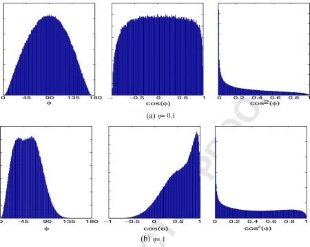
cos2_σ_{tumour area}

Fig. 2. The distributions of cossand cos2_s_{averaged over 10 subjects from the BraTS simulated images. The images were registered using a rigid transformation prior to}

com-putation and only the tumour areas were sampled. (a) shows the distribution of cossin the simulated tumour region. (b) shows the distribution of cossover the entire image. (c) shows the distribution of cos2_s_{proposed in}_Ref._[₂₀_{] in the simulated tumour region.}

[image:5.595.80.521.585.708.2]

(6)

UNCORRECTED

PR

OOF

661

662

663

664

665

666

667

668

669

670

671

672

673

674

675

676

677

678

679

680

681

682

683

684

685

686

687

688

689

690

691

692

693

694

695

696

697

698

699

700

701

702

703

704

705

706

707

708

709

710

711

712

713

714

715

716

717

718

719

720

721

722

723

724

725

726

727

728

729

730

731

732

733

734

735

736

737

738

739

740

741

742

743

744

745

746

747

748

749

750

751

752

753

754

755

756

757

758

759

760

761

762

763

764

765

766

767

768

769

770

771

772

773

774

775

776

777

778

779

780

781

782

783

784

785

786

787

788

789

790

791

[image:6.595.124.463.58.184.2]

792 Fig. 3. Example images of a T1-weighted brain containing a tumour area. The tumour areas are outlined in yellow in each image. Left: axial view. Middle: coronal view. Right: sagital view.(For interpretation of the references to colour in this ﬁgure legend, the reader is referred to the web version of this article.)

Formally, we assumethatD0(k) is a stationary random process y(t) with indextk∈R2_{, where}_∀_t_∼_U_{(0, 2p). We deﬁne the} ran-dom processz(t) = cosy(t) and thus∀trandom variableZ=z(t) has mean valueE_{Z_}= 0. In fact, by assuming mean ergodicity, we ﬁnd that

E_{Z_{} ∝}

z(t)dt_≡

R2

cos[D0(k)]dk= (1)

This is an important property for a similarity measure to be robust against occlusions. Since occlusions do not provide useful informa-tion for alignment, ideally they would be ignored. However, manual segmentation of occluded areas is time consuming and prone to error. Therefore, an ideal robust similarity measure would be able to automatically identify regions of the image that are occluding the true object of interest. Under the previous deﬁnition of robustness, the cosine similarity naturally represents a robust similarity measure as it automatically suppresses the contribution of outliers.

Given an image warping function with parametersp, maximising the sum of the cosine of orientation differences provides the robust similarity measure:

q=

k

cos

(

D0(k)[p]

)

(2)

For more details of the speciﬁcs of optimising (2) for image alignment, we refer the reader toRef.[16].

3.2. Cosine similarity in 3D

We make very similar assumptions for 3D images as we did in

Section 3.1for 2D images. We simply extend the previous notation by including the gradient of thez-axis, denoted asGi,z=Fz∗Ii. We also

redeﬁne the normalised gradient asg˜i(k) = g_g_ii(₍k_k)₎ wheregi(k)=

gi,x(k)2+gi,y(k)2+gi,z(k)2andgi(k) is deﬁned as the vector formed

by concatenating thex,yandzgradients together.

Measuring the angular distance between vectors in 3D is more complex than in 2D, due to the extra degree of freedom. In the fol-lowing sections, we describe two different measures that can be used to calculate similarities between vectors within 3D images, the spherical coordinates and the inner product. In the previous section, we described in detail how properties of the cosine of a uniform dis-tribution can be exploited to form a robust measure of similarity. The most important property was that uncorrelated areas such as occlu-sions should have no impact registration. This was formalised as the expectation of the sum of the uncorrelated elements should be zero. In the case of input to the cosine function, a given distribution must simply be symmetric over the positive and negative span of outputs

of the cosine. When symmetric over the positive and negative out-puts, the expectation of the cosine function is zero. In fact, we can relax the deﬁnition of a measure being robust to outliers by stating that we desire a measure whereby the expectation of the measure over image areas that are uncorrelated is zero.

In practise, when comparing two images where one image con-tains occlusions, there will be regions that are correlated and then the occluded region that is uncorrelated. In this case, the total dis-tribution of all pixels will be described by a mixture model of the occluded and non-occluded regions. We desire that the distribution of the uncorrelated areas has an expectation of zero and thus will not affect the optimisation of the similarity measure.

InSection 3.2.1 and Section 3.2.2we describe two measures of angular difference between 3D images. We investigate the distribu-tion of these angular measures when combined with the cosine func-tion and motivate that they are both suitable for use as a similarity measure between real 3D images.

3.2.1. Spherical coordinates

In 2D, a natural parametrisation of the angle between the two gradient vectors is the polar coordinate system. In 3D, we have three gradient vectors and thus require two angles to describe their orien-tation. Unlike in 2D, where the vectors lie on the unit circle, in 3D the vectors lie on the surface of a unit sphere. Therefore, it is possi-ble to parametrise the vectors in terms of the spherical coordinate system, which is described by two angles: the azimuth angle0with range [0, 2p) and the elevation anglehwith range [0,p]. Given the normalised gradients as vectors with Cartesian coordinates, we can calculate the spherical angles as follows:

ri(k) = ˜gi(k)= 1

0i(k) = arctan

˜ gi,y(k)

˜ gi,x(k)

hi(k) = arccosg˜i,z(k)

(3)

An illustration of the spherical coordinate system, as used in this paper, is given inFig. 1.

Our proposal is to combine the spherical coordinates with the cosine function in order to provide a robust similarity measure. Sim-ilar to the 2D case, we propose the cosine of azimuth differences, D0=01−02, and the cosine of elevation differences,Dh=h1−h2, as a combined similarity measures. Given a 3D image warping func-tion with parametersp, the spherical coordinates form a similarity measure as follows:

q=

k

cos

(

D0(k)[p]

)

+

k

cos

(

Dh(k)[p]

)

(4)

Optimisation ofEq.(2)is described in detail inSection 4.

(7)

UNCORRECTED

PR

OOF

793

794

795

796

797

798

799

800

801

802

803

804

805

806

807

808

809

810

811

812

813

814

815

816

817

818

819

820

821

822

823

824

825

826

827

828

829

830

831

832

833

834

835

836

837

838

839

840

841

842

843

844

845

846

847

848

849

850

851

852

853

854

855

856

857

858

859

860

861

862

863

864

865

866

867

868

869

870

871

872

873

874

875

876

877

878

879

880

881

882

883

884

885

886

887

888

889

890

891

892

893

894

895

896

897

898

899

900

901

902

903

904

905

906

907

908

909

910

911

912

913

914

915

916

917

918

919

920

921

922

923

924

[image:7.595.131.475.58.206.2]

(a)

(b)

Fig. 4. The mean distribution ofD0of the BraTS simulated images. The images were registered using a rigid transformation and only the tumour areas were sampled. (a) The distribution ofD0in the simulated tumour region. (b) The distribution ofD0over the entire image. It also shows the Laplacian distribution that best ﬁts the data.

Experimentally, we veriﬁed thatD0approximates a symmetric distribution for simulated tumour data taken from the Multimodal Brain Tumor Image Segmentation (BraTS) challenge, as shown in

Fig. 4.Fig. 4a shows the distribution ofD0between the tumour area circled in yellow inFig. 3and a healthy brain. The images were reg-istered using a rigid transformation beforeD0was computed. The azimuth angle is analogous to the angle studied in Ref.[34]and follows the same uniform distribution,D0∼U(0, 2p).

When the entire region of the rigidly registered brain images is considered, we ﬁnd that the distribution ofD0is clearly a mixture of two separate models, one for the occluded area and one for the rigidly registered area.Fig. 4b shows the distribution ofD0 calcu-lated over the entire image region of each image and a Laplacian distribution that best ﬁts the data. Thus, our experimental evidence suggests that the total distribution ofD0over the entire image region is a mixture model between a uniform distribution and a Laplacian distribution with approximately zero mean.

3.2.2. Inner product

A more general angular measure between two vectors is the inner product. Unlike inRef.[16]orSection 3.2.1, the inner product is a sin-gle ansin-gle and not the difference between two ansin-gles. Practically, the inner product measures the projection error between two vectors and is deﬁned as:

coss=g˜₁g˜2 (5)

In Ref. [34], the authors reasonably propose that the angle between the gradients of dissimilar images can take any value in [0, 2p) with equal probability. Similarly, the relationship between the gradient vectors of two dissimilar 3D images could feasibly be in any direction with equal probability. Therefore, the distribution of inner

products between two unrelated vectors can take the values [₋1, 1] with equal probability. Due to the expected range of inner product values, we would expect that cossfollows a uniform distribution, coss_∼U(₋1, 1). Note that this is a different assumption to that made inRef.[34], which assumes that theazimuth angle itself,D0, follows a uniform distribution. However, it is merely sufficient that the total sum of values from the dissimilar vectors is zero. Therefore, since E{U(−1, 1)}= 0, the inner product of normalised gradients satisfies our definition of being robust to outliers. InFig. 2a, we show that this assumption holds for the simulated tumour data taken from the BraTS challenge.

When the entire region of the rigidly registered brain images is considered, we ﬁnd that the distribution of cossis clearly a mixture of two separate models, one for the occluded area and one for the rigidly registered area.Fig. 2b shows the distribution of coss calcu-lated over the entire image region. In this case, the distribution of the inner product appears to be a mixture model between a uniform distribution and a zero mean Laplacian distribution. However, due to the ambiguity in the inner product in terms of orientation, the angle of the inner product is only deﬁned in the range [0,p] and thus only the positive tail of the Laplacian appears.

[image:7.595.131.470.603.727.2]

InFig. 2c we also show the distribution of the similarity measure proposed by Haber and Modersitzki[20]. InRef.[20], the authors propose the inner product as a similarity measure, which looks very similar to the measure we proposed in Eq.(5). However, Haber and Modersitzki[20]maximise the square of the inner product using a least squares Gauss–Newton optimisation. As we have shown, the inner product is related to the cosine between the vectors. Haber and Modersitzki[20]proposed the inner product squared as a similarity, which is equivalent to thesquare of the cosine. As we can see inFig. 2c, the cosine squared does not represent a symmetric distribution and therefore is not a robust similarity measure by our deﬁnition.

Fig. 5. Axial view of a T1-weighted brain images utilised for intensity inhomogeneity simulation. Left: original. Middle: with simulated bias ﬁeld applied. Right: bias ﬁeld.

(8)

UNCORRECTED

PR

OOF

925

926

927

928

929

930

931

932

933

934

935

936

937

938

939

940

941

942

943

944

945

946

947

948

949

950

951

952

953

954

955

956

957

958

959

960

961

962

963

964

965

966

967

968

969

970

971

972

973

974

975

976

977

978

979

980

981

982

983

984

985

986

987

988

989

990

991

992

993

994

995

996

997

998

999

1000

1001

1002

1003

1004

1005

1006

1007

1008

1009

1010

1011

1012

1013

1014

1015

1016

1017

1018

1019

1020

1021

1022

1023

1024

1025

1026

1027

1028

1029

1030

1031

1032

1033

1034

1035

1036

1037

1038

1039

1040

1041

1042

1043

1044

1045

1046

1047

1048

1049

1050

1051

1052

1053

1054

1055

1056

4. Robust Lucas–Kanade

Little work has been published on the applications of 3D Lucas–

Kanade (LK), despite the extension of LK into 3D being trivial[17]. Given the relative efficiency of Lucas–Kanade and other similar algo-rithms, and their potential accuracy under challenging conditions, we propose to investigate using LK for robust affine alignment in voxel images. To the best of our knowledge, this is the first such com-parison of using state-of-the-art LK fitting algorithms for voxel data. Given the similarity measures defined inSection 3, we propose novel LK algorithms that directly maximise the measures.

When referring to the operations performed by the LK algorithm we will use the following notations. Warp functions W(xi;p) =

[Wx(xi;p),Wy(xi;p),Wz(xi;p)] express the warping of the ith 3D

coordinate vector xi = [xi,yi,zi] by a set of parameters p =

[p₁,

. . .

,p_n] , wherenis the number of warp parameters. We extend the previously deﬁned linear indexkin to a coordinate vector,x= [x1,y1,z1,

. . .

,xD,yD,zD] that represents the concatenated vector of

coordinates, of lengthD, which allows the deﬁnition of a single warp for an entire image,W(x;p) = [Wx(x1;p),Wy(x1;p),Wz(x1;p), . . . ,

Wx(xD;p),Wy(xD;p),Wz(xD;p) ]. We assume that the identity warp

is found whenp = 0, which implies that_W(x_;0) = x. We abuse notation and deﬁne the warping of an imageIby parameter vec-torpasI(p) = I(W(x;p)), whereI(p) is a single column vector of concatenated pixels.

In the following sections we describe the details of relevant LK algorithms. We begin with the original forward additive LK algorithm[1,5]. We then describe the enhanced correlation coeffi-cient (ECC) algorithm[6]which was shown to be robust to inten-sity inhomogeneities. We conclude the existing algorithms with a description of the efficient inverse compositional algorithms for both the original LK method[35]and the ECC method[6]. Following the existing literature, we present our proposed LK algorithms. The first of which is a variation of the ECC method for normalised gradients and the second involves a traditional inverse compositional method. Both of the proposed algorithms take the inverse compositional form due to its computational efficiency.

4.1. Forward additive LK ﬁtting

The original forward additive

2LK algorithm[1,5]seeks to min-imise the sum of squared differences (SSD) between a given template image and an input image by minimising the sum of the squared pixel differences:

argmin

p

I(p)₋T(0)2 ₍₆₎

whereT(0) is the unwarped reference template image. Due to the non-linear nature ofEq.(6)with respect top,Eq.(6)is linearised by taking the ﬁrst order Taylor series expansion. By iteratively solving for some smallDpupdate top, the objective function becomes

argmin

p

I(p) +∇I

∂

W

∂

pDp−T(0)

2 ₍₇₎

where_∇Iis the gradient over each dimension ofI(p) warped into the frame ofTby the current warp estimateW(x;p). ∂W

∂p is the Jacobian of the warp and represents the ﬁrst order partial derivatives of the warp with respect to each parameter.∇I∂W

∂p is commonly referred to as the steepest descent images. We will express the steepest descent images as ∂_∂I(_pp). Eq. (7)is now solvable by assuming the

Gauss–Newton approximation to the Hessian,H=

∂I(p) ∂p

:

Dp=H−1

∂

I(p)

∂

p [T(0)−I(p)] (8)

Eq.(8)can then be solved by iteratively updatingp_←p+Dpuntil convergence.

4.2. ECC LK ﬁtting

The enhanced correlation coeﬃcient (ECC) measure, proposed by Evangelidis and Psarakis[6], seeks to be invariant to illumination differences between the input and template image. This is done by suppressing the magnitude of each pixel through normalisation. In

Ref.[6], they provide the following cost function

argmax p

I(p) T(0)

I(p)T(0) (9)

Assuming a delta update as before and linearising in a similar manner toEq.(7)results in

argmax p

ˆ T I(p) +

∂I(p) ∂p Dp

I(p) +∂_∂I(_pp)Dp (10)

whereTˆ = T(0)

T(0). Evangelidis and Psarakis[6]give a very com-prehensive proof of the upper bound of Eq.(10), which yields the following solution forDp

Dp=H−1

∂

I(p)

∂

p

I(p)2₋_I₍_p₎ _Q_I₍_p₎

ˆ

T I(p)− ˆT QI(p)

ˆ T−I(p)

(11)

whereQis an orthogonal projection operator on the Jacobian,J= ∂I(p)

∂p , deﬁned asQ=J(J J)−1J .

In fact, theDpupdate given inRef.[6]is more complex than

Eq. (11), as it seeks to ﬁnd an upper bound on the correlation between the two images. However, in the case whereEq.(11)does not apply, it is unlikely that the algorithm is able to converge. For this reason, we only consider the update equation presented inEq.(11).

4.3. Inverse compositional LK

The inverse compositional algorithm, proposed by Baker and Matthews[35], performs a compositional update of the warp and linearises over the template rather than the input image. Lineari-sation of the template image causes the gradient in the steepest descent images term to become fixed. The compositional update of the warp assumes linearisation of the term ∂W_∂(_px;0), which is also fixed. Therefore, the entire Jacobian term, and by extension the Hes-sian matrix, are also fixed. Similar to the

2SSD algorithm described inSection 4.1, we pose the objective function as:

argmin

p T(Dp)−I(p)

2 ₍₁₂₎

where we notice that the roles of the template and input image have been swapped. Assuming an inverse compositional update to the warp,W(x;p)←W(x;p)◦W(x;Dp)−1_{and linearisation around the} template,Eq.(12)can be expanded as:

argmin

p I(p)−

∂

T(0)

∂

p Dp−T(0)

2 ₍₁₃₎

(9)

UNCORRECTED

PR

OOF

1057 1058 1059 1060 1061 1062 1063 1064 1065 1066 1067 1068 1069 1070 1071 1072 1073 1074 1075 1076 1077 1078 1079 1080 1081 1082 1083 1084 1085 1086 1087 1088 1089 1090 1091 1092 1093 1094 1095 1096 1097 1098 1099 1100 1101 1102 1103 1104 1105 1106 1107 1108 1109 1110 1111 1112 1113 1114 1115 1116 1117 1118 1119 1120 1121 1122 1123 1124 1125 1126 1127 1128 1129 1130 1131 1132 1133 1134 1135 1136 1137 1138 1139 1140 1141 1142 1143 1144 1145 1146 1147 1148 1149 1150 1151 1152 1153 1154 1155 1156 1157 1158 1159 1160 1161 1162 1163 1164 1165 1166 1167 1168 1169 1170 1171 1172 1173 1174 1175 1176 1177 1178 1179 1180 1181 1182 1183 1184 1185 1186 1187 1188 Solving forDpis identical toEq.(8), exceptthatthe Jacobian and

Hessian have been pre-computed

Dp=H−1

∂

T(0)

∂

p [I(p)−T(0)] (14)

The ECC can also be described as an inverse compositional algorithm, by performing the same update to the warp and simply swapping the roles of the template and reference image. In short, solving ECC in the inverse compositional case becomes

Dp=H−1

∂

Tˆ

∂

p

ˆT2_{− ˆ}_T _Q_Tˆ

I(p) Tˆ₋I(p) QTˆI(p)− ˆT

(15)

whereQis as before, exceptJ= ∂_∂T_pˆ. Any term involvingTˆ is ﬁxed and pre-computable, so the reduction of calculations per-iteration is substantial.

It is worth noting that not every family of warps is suitable for the inverse compositional approach. The warp must belong to a family that forms a group, and the identity warp must exist in the set of possible warps. For more complex warps, such as piecewise aﬃne and thin plate spline warping, approximations to the inverse compositional updates have been proposed[36,37].

4.4. Inner product ECC LK

Given the inner product similarity measure as described in

Section 3.2.2, we seek to embed it within the LK framework in order to present a robust parametric alignment algorithm. Therefore, we begin by restating our cost function:

argmax p

k

cos

(

s(p)

)

(16)

with an abuse of notation for the parameters which are hidden within the cosine function. ExpandingEq.(16)reveals the parame-ters and makes the relationship between our inner product similarity and the ECC framework clear:

argmax

p ˜

gI(p) g˜T(0) (17)

which yields our forward additive algorithm.

However, unlike in ECC where the vectors represent concatenated normalised intensities, we are considering normalised gradients. Since gradients have three separate components we must consider the derivatives when linearisingg_I. Sinceg_Iis composed of multiple components, there will be extra derivatives to calculate via the chain rule. Formally, linearisingEq.(17)with respect togIyields

argmax

p g˜T

˜

gI(p) +JgDp

˜gI(p) +JgDp

(18)

whereJ_gis the matrix formed by correctly computing the derivative ofg_Iwith respect to each component ofg_I. For example, given that

gI,x(p) is a vector formed of thex-components of the gradients and

˜

gI,x(p) is a vector formed ofg˜I,x(p)[k] =g_gI,_Ix₍(_pp_)[)[_kk_]], the true derivative

ofg˜I,x(p) is

∂

g˜I,x(p)

∂

p =

∂

g˜I,x(p)

∂

gI,x(p)

∂

gI,x(p)

∂

p

∂

g˜I,x(p)

∂

gI,x(p)

= gI,y(p) 2₊_g

I,z(p)2

gI,x(p)2+gI,y(p)2+gI,z(p)23/2

(19)

where∂gI,x(p)

∂p is equivalent to ∂I(p)

∂p in the original ECC equations. The

yandzderivatives are given in a similar fashion as

∂

g˜I,y(p)

∂

gI,y(p)

= gI,x(p) 2₊_g

I,z(p)2

gI,x(p)2+gI,y(p)2+gI,z(p)2

3/2

∂

g˜I,z(p)

∂

gI,z(p)

= gI,x(p) 2₊_g

I,y(p)2

3/2 (20)

However,∇g_I_,_x, formally the image gradient, represents the gradient over only thex-component, and is equivalent to the second order derivative of the gradients with respect tox.

Since ∂gI,x(p)

∂p is a matrix and ∂g˜I,x(p)

∂gI,x(p) is a vector, we multiply the

two using a Hadamard product, denoted by theoperator. How-ever,∂g˜I,x(p)

∂gI,x(p)must ﬁrst form a matrix,Jx, of sizeD×pby repeating the

vectorptimes to form columns within the matrix. Finally the total x-component Jacobian is given byJg,x=Jx∂gI_∂,x_p(p).

Given thatJ_g_,_i∀i ∈ {x,y,z}have been calculated, the total deriva-tive term is given by Jg = [Jg,x,Jg,y,Jg,z] . Solving for Dp is now

identical to the ECC formulation:

Dp=H−1_J g

gI(p)2−gI(p) QgI(p)

˜

g_TgI(p)− ˜gTQgI(p)

˜

gT−gI(p)

(21)

Since the update step is identical to the one given inEq.(15)it is simple to reformulate the inner product ECC in an inverse

composi-Q3 tional form by following a derivation identical toSection 4.3. In the

Experimentssection, we consider the inverse compositional form of the algorithm.

4.5. Spherical SSD LK

In contrast to the inner product derivation in the previous section, the spherical representation requires the optimisation of the sum-mation of two cosine correlations. In theory, it would be possible to solve for each correlation separately in a manner similar to that proposed by Tzimiropoulos et al. [16]. This would be suboptimal as it would require an alternating optimisation scheme. Therefore, in the interest of solving a single objective, we note the following relationship between the two summations:

argmax p

k

cos

(

D0(p)

)

+

k

cos

(

Dh(p)

)

(22)

is equivalent to the minimisation of

argmin p ⎛ ⎜ ⎜ ⎝

cos0I(p)

sin0I(p)

coshI(p)

sinhI(p)

⎞ ⎟ ⎟ ⎠− ⎛ ⎜ ⎜ ⎝

cos0T(0)

sin0T(0)

coshT(0)

sinhT(0)

⎞ ⎟ ⎟ ⎠ 2 argmin p ⎛ ⎜ ⎜ ⎜ ⎝ ˜

gI,x(p)

˜

gI,y(p)

˜

gI,z(p)

1− ˜g2

I,z(p)

⎞ ⎟ ⎟ ⎟ ⎠− ⎛ ⎜ ⎜ ⎜ ⎝ ˜

gT,x(0)

˜

gT,y(0)

˜

gT,z(0)

1− ˜g2

T,z(0)

⎞ ⎟ ⎟ ⎟ ⎠ 2 (23)

where sinh∗(•) =1− ˜g2

∗,z(•) where * denotes either the template

or the input image. For notational simplicity, letsz˜(•) =1_{− ˜}g2

z(•).

We deﬁne the forward additive objective function as

argmin

p ˆgI(p)− ˆgT(0)

2 ₍₂₄₎

(10)

UNCORRECTED

PR

OOF

1189

1190

1191

1192

1193

1194

1195

1196

1197

1198

1199

1200

1201

1202

1203

1204

1205

1206

1207

1208

1209

1210

1211

1212

1213

1214

1215

1216

1217

1218

1219

1220

1221

1222

1223

1224

1225

1226

1227

1228

1229

1230

1231

1232

1233

1234

1235

1236

1237

1238

1239

1240

1241

1242

1243

1244

1245

1246

1247

1248

1249

1250

1251

1252

1253

1254

1255

1256

1257

1258

1259

1260

1261

1262

1263

1264

1265

1266

1267

1268

1269

1270

1271

1272

1273

1274

1275

1276

1277

1278

1279

1280

1281

1282

1283

1284

1285

1286

1287

1288

1289

1290

1291

1292

1293

1294

1295

1296

1297

1298

1299

1300

1301

1302

1303

1304

1305

1306

1307

1308

1309

1310

1311

1312

1313

1314

1315

1316

1317

1318

1319

1320 where gˆI(p) = g˜I,x(p),g˜I,y(p),g˜I,z(p),g˜I,sz(p) and gˆT(0) =

˜

gT,x(0),g˜T,y(0),g˜T,z(0),g˜T,sz(0) , the concatenated vectors of each

normalised component.

Similar to the derivation inSection 4.4, the Jacobian must be taken over each component and thus linearising aroundgˆI(p) yields

argmin

p ˆgI(p) +

ˆ

JgDp− ˆgT(0)2 (25)

whereˆJg=

ˆ

Jg,x,ˆJg,y,ˆJg,z,ˆJg,sz

. Unlike inSection 4.4, the calculation of each Jacobian is not identical due to the different normalisation procedure taken for each component. Given that we can split the par-tial derivativeJg,x =Jx∂g_∂I,x_p(p), we deﬁne the component speciﬁc

Jacobian,J_i_∀i_{∈ {}x,y,z,sz_}as:

Jx=

gI,y(p)2

Jy=

gI,x(p)2

Jz=

gI,x(p)2+gI,y(p)2

Jsz=−

gI,z(p)

gI,x(p)2+gI,y(p)2

3/2

gI,x(p)2+gI,y(p)2

(26)

Now, given the deﬁnitions of the correct Jacobians per component, we can solveEq.(25)as:

Dp=H−1ˆ_J g

_ˆ

gT(0)− ˆgI(p) (27)

Given that the update inEq.(27)is identical to that ofEq.(8), it would be trivial to formulate an inverse compositional form of this residual by following the steps described inSection 4.3.

5. Robust nonrigid alignment

Non-rigid registration is the term generally used to describe an alignment algorithm that utilises a non-rigid warp. A non-rigid warp is generally achieved via a motion model that allows for smaller scale local deformations than can be achieved under models such as aﬃne or similarity. For example, Rueckert et al.[26]proposed free-form deformations (FFD) as a motion model that gives a smooth spline-based transition between neighbouring control points. How-ever, due to the local nature of non-rigid alignment algorithms, they require many more parameters. In the case of FFDs there may be many thousands of parameters depending on the resolution of the FFD chosen. Unfortunately, due to the complexity of the parameter space, this causes Gauss–Newton algorithms such as those described inSection 4to be infeasible. This is primarily due to the fact that the size of the Hessian matrix is deﬁned by the number of parameters and a large Hessian matrix may be non-invertible under reasonable memory requirements.

Therefore, we augment the FFD algorithm given inRef.[26]to use our similarity measure. The local transformation described by a FFD consists of a mesh of control points,0i,j,k, separated by a uniform

spacing. The FFD is then given as inRef.[26], as a 3-D tensor product of 1-D cubic B-splines

W(x;p)_local= 3

l=0 3

m=0 3

n=0

Bl(u)Bm(v)Bn(w)0i+l,j+m,k+n (28)

whereBl describes thelth basis function of the B-spline,B0(u) = (1−u)3

_/

_6,_B

1(u) = (3u3−6u2+ 4)

/

6,B2(u) = (−3u3+ 3u2+ 3u+ 1)

/

6,B3(u) =u3

/

6 andi,jandkare control point indices over thex, yandzaxis respectively. We then perform a simple gradient descent algorithm, which terminates when a local minima is reached.

Typically, the total cost function for the FFD algorithm consists of a similarity term that depends in the data and a regularisation term that enforces smoothness on the local transformation. In this work we seek to improve the performance of the similarity term in the presence of systematic errors.

Let us assume that the parameters of the FFD areV = _{0i,j,k}.

We replace the normalised mutual information similarity measure C(V)Similarity from the original FFD algorithm with our new robust similarity. For example, for the inner product similarity as described inSection 3.2.2we deﬁneC(V)IPas

C(V)IP=g˜I(V) g˜T(0) (29)

The parameters,V, can then be updated in gradient descent form as follows:

V=V+l ∇VC(V)IP

∇VC(V)IP

(30)

where∇VC(V)IPis the gradient of the similarity measure.

5.1. Numerical stability

As discussed inRef.[20], it is not possible to use normalised gradient ﬁelds directly due to discontinuities in differentiation. We thus regularise the normalised gradient ﬁelds using the technique presented inRef.[23].

C(V)IP=

k∈Y

gI(V)[k] gT(0)[k] +3t

gI(V)[k]3gT(0)[k]t

(31)

where •_∗₌•_,•₊∗2_and_Y_{is the set of indices} correspond-ing to the target image support. In this work3andtrequire only a single parameter, as opposed to the user speciﬁed regularisation val-ues chosen inRef.[23]. Explicitly,3andtare computed following an automatic choice based on total variation

3= g VI

k∈YI

gI(V)[k], t=

g VT

k∈YT

gT(0)[k] (32)

whereg

>

0 is a parameter for noise ﬁltering andV*is the volume of interest in the image domainY*.

5.2. Robustness against bias ﬁelds

In this section we provide a formal proof of the robustness of our cost functions to bias ﬁeld corruption. Consider an image signalM with no intensity inhomogeneities and a smooth signalQ, represent-ing a multiplicative bias ﬁeld[38,39]. We assumeQto be constant within a small neighbourhood,N(k) = (DkxDkyDkz). Therefore, for

Dkx, we have

I(k) =M(k)Q(k) +4

I(k+Dkx) =M(k+Dkx)Q(k+Dkx) +4 (33)