Bayesian deconvolution of vessel residence time distribution

Revised submission to IJCRE 2017-08-29 Accepted 2017-10-09

Bayesian Deconvolution of Vessel Residence Time Distribution

Thomas Huddle1, Paul Langston2*, Edward Lester1

1. Advanced Materials Research Group; 2. Fluids & Thermal Engineering Group; Faculty of Engineering, University of Nottingham, Nottingham, NG7 2RD, United Kingdom

Abstract

Residence time distribution (RTD) within vessels is a critical aspect for the design and operation of continuous flow technologies, such as hydrothermal synthesis of nanomaterials (Cabanas, Darr et al. 2000). RTD affects product characteristics, such as particle size distribution. Tracer techniques allow measurement of RTD, but often cannot be used on an individual vessel in multiple vessel systems due to unsuitable exit flow conditions. However, RTD can be measured indirectly by removal of this vessel from the system and deconvoluting the resulting detected tracer profile from the original trace of the entire system.

This paper presents three models for deconvolution of RTD: BAY an application of the Lucy-Richardson iterative algorithm (Lucy-Richardson 1972, Lucy 1974) using Bayes’ Theorem, LSQ an adaptation of a least squares error approach (Blackburn 1970) and FFT a Fast Fourier Transform. These techniques do not require any assumption about the form of the RTD.

The three models are all accurate in theoretical tests with no simulated measurement error. For scenarios with simulated measurement error in the convoluted distribution, the FFT and BAY models are both very accurate. The LSQ model is the least suitable and the output is very noisy; smoothing functions can produce smooth curves, but the resulting RTD is less accurate than the other models.

In experimental tests the BAY and FFT models produce near identical results which are very accurate. Both models run quickly, but in real time control the runtime for BAY would have to be considered further. BAY does not require any filtering or smoothing here, and so potentially there are applications where it might be more useful than FFT.

Keywords: Residence Time Distribution; Deconvolution; Bayes’ Theorem; Least Squares; FFT

1Introduction

Levenspiel (Levenspiel 1999) describes deviations from ideal flow (plug or mixed) for process equipment such as reactors, heat exchangers, packed columns caused by channelling, recycling of flow, stagnant regions which can adversely affect performance, costs or product quality. Deconvolution of residence time distribution (RTD) from tracer signals flowing into and out of such equipment can be very useful in design optimisation and control.

Langston (Langston 2002) describes practical cases where the properties of a system are a complex mixture of several components. It is often useful to extract component compositions from system property measurements; such as in signal processing, coal blend analysis and measurement of particle size distribution. Vessels in series will also give rise to convoluted RTD’s. Accurate deconvolution of individual vessel features is a challenging process.

An important application concerns residence time distribution measurements of reactors in continuous flow processes. In these systems the reactor is defined as the primary system volume in which the desired chemical transformation takes place. Often there will be more than one chemical reaction occurring at the required conditions, such as competing reactions or decomposition of the product. The various reaction pathways are dependent on the reaction parameters, which include residence time in the reactor; based on an understanding of the various pathway kinetics, optimal processing conditions usually requires a specific residence time with minimal distribution. Jumbam (Jumbam, Skilton et al. 2012) have demonstrated the ability to optimise the methylation of alcohols in continuous flow supercritical carbon dioxide; the yield and selectivity are shown to depend on residence time among other reaction parameters. Another practical example is the continuous hydrothermal synthesis of nanomaterials in supercritical fluids; Adschiri (Adschiri, Hakuta et al. 2001) first proposed a mechanism for the generation of metal oxides using this technique. With countless applications, the properties of nanomaterials are greatly influenced by particle size, which is often in turn dictated by residence time in the system reactor. For many nanomaterial species where nucleation is virtually instantaneous, particle growth can be directly related to time spent in the reactor, as studied by various groups including Norby (Norby, Jensen et al. 2013); thus the residence time distribution in the reactor will directly translate to particle size distribution in the product solution. The use of different reactor geometries by Blood (Blood, Denyer et al. 2004) for continuous hydrothermal nanomaterial synthesis have been investigated previously and it is well known that mixing dynamics has a significant impact on particle nucleation and growth. In addition to reactor design issues, other control variables for this continuous hydrothermal process were discussed by Lester (Lester, Aksomaityte et al. 2012), including temperature, flow rate, flow ratio, pipe diameter and pressure. A recent project scales this process from bench to pilot through to industrial scale, at over 100 tons per year capacity, with the FP7 Sustainable Hydrothermal Manufacturing of Nanomaterials (SHYMAN) project (Particles 2015, Shyman 2015). Better control of products from this process, and the inevitable changes in product quality (as a result of scaling the process) will become a focus for the industry and therefore understanding residence time distributions and mixing dynamics is essential.

found. Simmons (Simmons, Langston et al. 1999) used a similar technique to predict particle size distribution from chords that was partially successful.

Least squares methods were used in the following RTD analysis. Kuu (Kuu 1992) used a numerical deconvolution method with Powell's non-linear least-squares algorithm to search for values of dispersion coefficients of solute molecules in a drug delivery system. Bruce (Bruce, Sai et al. 2004) experimentally measured the RTD in a turbulent bed contactor in series with an ideal Mixed Flow Tank. The RTD of the ideal mixed flow tank was deconvoluted from the RTD of the entire system to obtain the RTD of turbulent bed contactor alone as a function of Peclet number and mean residence time of an axial dispersion model; optimal values were found using a Matlab-based least squares function. Boskovic (Boskovic and Loebbecke 2008) modelled RTD in micromixers; deconvolution involved minimization of sum of error square by the unconstrained quasi-Newton method; two flow models were developed, one based on axial dispersion, the other based on statistical distributions allowing a certain skewness; the latter gave a better fit to the range of their experiments. Adeosun (Adeosun and Lawal 2009)

describes numerical and experimental mixing studies in a flow micromixer and used the convolution–deconvolution technique, in which time–domain curve fitting via non-linear optimization was used to estimate parameters in the RTD model.

The Fast Fourier Transform FFT has been used in RTD analysis. Viitanen (Viitanen 1997) applied a FFT to deconvolute RTDs of process equipment with examples from aquifers in bedrock and industrial equipment with recirculation; this method allows filtering in the frequency domain of data with poor statistics. Gooseff (Gooseff, Benson et al. 2011) estimated RTDs in stream surface transient storage zones via signal deconvolution with Fourier and Laplace transforms.

A method to estimate RTD in complex systems is to use a Bayesian approach with a Markov Chain Monte Carlo model to infer presumed RTD form parameters. Krone-Davis (Krone-Davis, Watson et al. 2013) analysed pesticide reduction in constructed wetlands using a tanks-in-series model. Massoudieh (Massoudieh, Leray et al. 2014) characterised groundwater flow systems using transient environmental tracer data.

Langston (Langston, Burbidge et al. 2001) used Bayes’ theorem iteratively to predict diameter distributions of spherical particles or droplets from measurements of chords. It was then further developed (Langston and Jones 2001) to analyse non-spherical shapes in 2D; (Langston 2002) developed the model for general cases of component mixture deconvolution and theoretically compared it to a least squares method. The latter was shown to be generally more applicable and robust, but the Bayes’ model was, in some cases, less susceptible to simulated noise. Subsequent to publication of these papers the authors found a similar method in the Lucy-Richardson algorithm (Lucy-Richardson 1972, Lucy 1974) developed for image analysis.

2Models of RTD Deconvolution

2.1Vessel RTD Convolution

Levenspiel (Levenspiel 1999) describes how the residence time distribution of a fluid passing through a vessel can be normalised and represented by E the exit age distribution for a closed vessel boundary condition (fluid only enters and leaves vessel once). A one-shot tracer signal entering (Cin) and leaving a vessel (Cout) can be represented by the convolution integral

' ' 0 '

)

(

)

(

)

(

t

C

t

E

t

t

dt

C

t

in

out







in

out

E

C

C



If we have three independent flow units a, b, c, closed and connected in series then

in c b a

out

E

E

E

C

C



Levenspiel (Levenspiel 1999) describes that independence implies that a fluid loses its memory between vessels and if an element flows faster in one vessel it is no more likely to flow faster in the next vessel, which is not always the case with laminar flow.

Section 2 now describes how deconvolution of RTD can be undertaken using either:  Bayes’ Theorem – model referred to later as BAY

 Least Squares - LSQ

 Fast Fourier Transform - FFT  Polynomial Division.

2.2RTD Deconvolution using Lucy-Richardson algorithm model BAY

A far more challenging exercise is deconvolution; ie if Cout, Cin, Ea, Eb, are known then

calculate Ec. This can be more generally represented by a two-vessel system: say Eb is

unknown, Ea and ET are known,

b a

T

E

E

E



Lee (Lee 2012) describes Bayes’ theorem as follows. If A1,…,Am are a set of mutually

exclusive, exhaustive events in a possibility space Sp, and B is any other event in Sp such that P(B)>0, then

m j A P A B P A P A B P B A P _m k k k j j

j 1,2,...,

This is applied here using the iterative procedure used in image analysis (Richardson 1972, Lucy 1974) and modified for estimating diameter distributions form chord measurements (Langston, Burbidge et al. 2001).

Dividing E into N equal time bins j:

1 Assume a uniform distribution in Ebj = 1.0/N, for all j (or input an initial estimate)

2 For each j use Bayes’ theorem to calculate probability Pji equivalent to EbjTi, which

can be considered as probability that a fluid element which exits total system at time bin i resided in vessel b for j time bins



for each i

)

1

(







E

i

j

E

3 For each j recalculate (note denominator equals unity)





4 If Eb has changed significantly repeat from step 2 using the new values of Eb; however,

in this paper the model is run for a specified number of iterations, nitr.

It is noted here that E is being used in a discretized form representing bin probabilities rather than a continuous probability density (hence the +1 in step 2 above); this is also applicable to the RTD plots shown later.As indicated above, for Bayes’ theorem to be applicable the flow units must be independent. The time interval (bin size) must also be small relative to the overall time.

2.3RTD Deconvolution using Least Squares model LSQ

Blackburn (Blackburn 1970) describes the problem in spectral analysis as follows:



jR e S

X

1

i = 1,….,n

Si is the amplitude of the data spectrum at the ith channel or sample point Rij is the amplitude of the jth reference spectrum at the ith channel Xj is the set of coefficients to be extracted

ei is the noise or error spectrum n is the number of channels

m is the number of standards.

Summing over the n channels obtains  the sum of the error squares. A least-square error approach based on calculating (d/dXk) for k = 1,.., m, gives a set of m linear equations of the

form: j m j n i ik ij n i ik

i

R

R

R

X

S

_

























 



1 1 1

These can be solved to give optimal Xj values. This requires a matrix Rij , but we have a vector

for each vessel RTD. Hence the model is applied here to a two vessel deconvolution by formulating Rij from the vector Ea:

Rij = Eak, where k=i – j +1 and k >0 and k < N+1 , else Rij =0

where i is the subscript of ET (=S above) and j is the subscript of Eb (=X above).

The output from this model is generally very noisy here. Integral smoothing functions available in Matlab were investigated. General smoothing algorithms such as the default moving average or Savitzky-Golay filters, are not well suited, regardless of the polynomial degree specified, as the noise on the response data appears to be equal across all time bins (including where the probability of Eb is actually zero). Smoothing which operate on localised ranges of time bins

appear more useful. The most accurate was found to be a local regression method using weighted linear least squares and a 2nd degree polynomial model (‘loess’ in Matlab); this method is implemented using the Matlab smooth function with the ‘loess’ method, with optimal

values for the span parameter varying between 0.2 and 0.5 and the function is applied twice in a loop; additionally, any negative values for the LSQ result are set to zero, although this makes little difference to the overall accuracy.

2.4RTD Deconvolution using Fast Fourier Transform model FFT

As noted in section 1 Viitanen (Viitanen 1997) applies FFT to deconvolute RTDs of process equipment. In the frequency domain w the convolution becomes a straightforward multiplication and the deconvolution a division.

)

(

).

(

)

(

w

E

w

E

w

E



)

(

/

)

(

)

(

w

E

w

E

w

Eb(t) can then be obtained by the inverse FFT after appropriate filtering in the frequency

domain to account for measurement error. This method is applied here using Matlab functions. The filtering at high and low frequencies (see code on-line) is essential here. Also truncating any values below zero improved the performance of the model here.

2.5RTD Deconvolution using Polynomial Division

RTD deconvolution is similar in principle to a more general vector deconvolution. The function in Matlab deconv does this by polynomial division. This has been tested here for RTD deconvolution; it is accurate for theoretical cases but is highly inaccurate in practice with measurement errors; in this study the method even failed to produce meaningful results with practical or simulated measurement error. This reason is clear on considering the principle of the method where errors in the coefficients of the higher terms are propagated in sequential division. Hence it is concluded that it is not worth considering this method further here.

2.6Measures of Accuracy

To assess the models the deconvoluted RTD is compared with the known RTD using three methods:

 Mean Square Error MSE

 Coefficient of Determination R2

 Overlapping Coefficient OVL (Clemons and Bradley 2000)

𝑀𝑆𝐸 =

1

𝑁∑(𝐸𝑖 − 𝐸𝑏𝑖)2

𝑁

𝑖=1

Where Ei is the estimated probability for each bin, Ebi is the known target probability for each

corresponding bin, and N is the total number of bins.

𝑅2 _{= 1 −} ∑𝑁𝑖=1(𝐸𝑖 − 𝐸𝑏𝑖)2

∑𝑁 (𝐸_𝑏𝑖 − 𝐸̅̅̅̅)_𝑏𝑖 2 𝑖=1

𝑂𝑉𝐿 = ∑ min [𝐸𝑖, 𝐸𝑏𝑖] 𝑁

3Application of RTD Deconvolution

3.1Theoretical Examples

3.1.1Theoretical case with no Simulated Measurement Error

Levenspiel (Levenspiel 1999) describes types of flow models: the dispersion model and tanks-in-series model which are similar and widely applicable, and the pure convection model for laminar flow in short pipes. For simplicity initial theoretical tests were undertaken on deconvolution of two normal distributions with no simulated measurement error. All the models, BAY, LSQ and FFT are accurate in these tests.

In order to investigate the potential accuracy of the models when tackling the deconvolution of non-normal convoluted data, as found in our reactor systems, two theoretical “shouldered” distributions were generated through the additive combination of normal distributions with differing parameters. These simulated examples more closely represent practical distributions generated for tubular reactor residence times, where tailing of the peaks is a common feature.

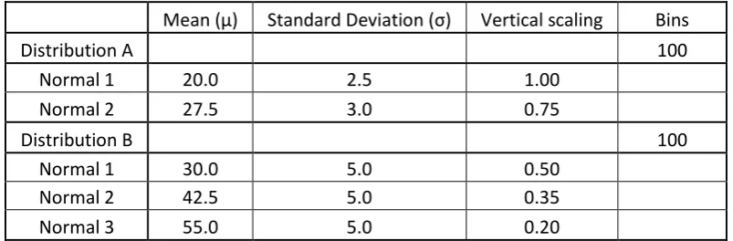
In generating the shouldered distributions, the underlying normal distributions were subjected to a vertical scaling factor in order to control their influence on the combined distribution; the resultant shouldered distributions were then converted to probability distributions through division by their total integral. Distribution A was generated by the additive combination of two normal distributions, and distribution B from three normal distributions using the parameters indicated in Table 1.

Table 1: Parameters used to produce realistic distributions A and B; then converted into bin probabilities Ea and Eb.

Mean (μ) Standard Deviation (σ) Vertical scaling Bins

Distribution A 100

Normal 1 20.0 2.5 1.00

Normal 2 27.5 3.0 0.75

Distribution B 100

Normal 1 30.0 5.0 0.50

Normal 2 42.5 5.0 0.35

Normal 3 55.0 5.0 0.20

The probability distributions for A and B (Ea and Eb) are plotted along with that of the

convolution of A and B (Et) in Figure 1 with a time bin size of 1s. Figure 2 illustrates successive

iterations of the BAY model in deconvoluting Ea from ET in order to generate an estimate of Eb; the true value of Eb and the estimate from the model are graphically indistinguishable after

Figure 1: Input probability distributions Ea and Eb produced from theoretical

non-normal distributions, and their convoluted product ET

Figure 2: Plot of the Bayes iterative approximations of Eb, represented as En;curves for

Eb and for the BAY nitr =100 estimate are graphically colinear in this theoretical no error

Table 2: Model accuracy in calculation of RTD of B for theoretical case with no replicated measurement error

MSE R2 OVL

BAY nitr =10 8.4e-7 0.9949 0.9748

BAY nitr =100 3.8e-9 1 0.9984

BAY nitr =1000 4.1e-11 1 0.9998

LSQ 7.3e-7 0.9956 0.9709

FFT 9.2e-13 1 1

3.1.2Case of non-Normal Distribution with Simulated Measurement Error

In practical scenarios, experimental inaccuracy and bias may produce error in any measured residence time. In order to evaluate the effect on the deconvolution method, simulated error has been applied to the convoluted distribution generated using the parameters detailed in section 3.1.1. The probability distribution Ea can then be deconvoluted from the erroneous

distribution ET-err in order to observe the effect on the estimation of Eb.

Several types of error are observed in practice: a bias, i.e. shifting the distribution by a fixed time; noise in the distribution, resultant of detector issues (when measuring residence time by tracer detection); scaling of the distribution, i.e. compression or expansion of the distribution resulting in a similar shape, but occurring over a different range of time (pump flow rate inaccuracies/inconsistencies).

Unpublished work within the Lester group involving the injection and detection of tracers has shown the last of these error types (scaling) to be most frequently observed. Figure 3 illustrates an example of a simulated “scaling error” applied to ET, with 10% compression scaling applied

about the bin at which the probability of ET is at maximum, in order to generate ET-err. The

Figure 3: Input probability distributions, with time bin of 1s, Ea and Eb used to produce

ET. ET has then been subjected to compression scaling by 10 % about the bin of its

maximum probability to generate ET-err. This is reasonably similar to frequently observed

experimental error.

Table 3: Model accuracy in calculation of RTD of B (Eb) for theoretical case with

simulated 10% compression of AB (ET-err) to replicate measurement error

MSE x10-6 R2 OVL

BAY nitr =10 5.79 0.9648 0.9267

BAY nitr =100 5.36 0.9673 0.9314

BAY nitr =1000 5.34 0.9674 0.9315

LSQ 16.3 0.9007 0.8736

FFT 5.04 0.9692 0.9346

SEE OVERPAGE FOR FIGURE

Figure 4: Plots comparing BAY nitr =100, LSQ and FFT methods for approximating B

The FFT and BAY models are both very accurate, with FFT marginally the best. 10 iterations for the BAY model seems sufficient for practical purposes. The LSQ model is the least suitable; Matlab produces a warning message on solution of the matrix equation Matrix is close to singular or badly scaled, and the output is very noisy; smoothing functions can produce smooth curves, but the resulting RTD is less accurate than the other two models. (Further investigation for zero replicated error cases, not shown here, indicates that LSQ is accurate, not noisy and no smoothing is required for about 40 or fewer time bins in Ea and in Eb.) Further investigation

is required to test if this method could be improved, it is not considered further in this paper.

3.2Experimental Examples

3.2.1Experimental Method

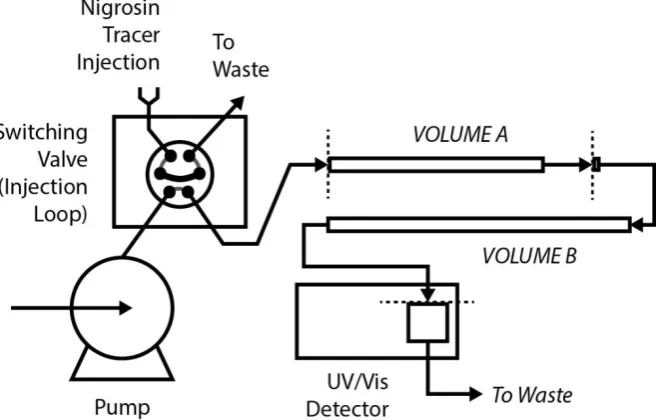
Figure 5: Diagram showing the apparatus configuration used for measuring residence time distributions inside volumes A and B. The “inj” volume can be considered as the above system without A and B present.

When instructed by the computer script, the valve switches to the “inject” position, which would introduce the fixed volume of tracer solution into the system at the predetermined flow rates. After passing through the system volumes of interest, the concentration of tracer detected at the system outlet was continuously measured using a Gilson 119 UV/vis detector, set to monitor at a wavelength of 545 nm (visible).

The system volume was divided into two sections, referred to as sections A and B. The primary volume of section A was a 200 mm length of stainless steel tubing (0.25” outer diameter, 2.34 ml volume) and section B a 300 mm length of the same tubing (3.51 ml volume). Both volumes also included short sections of 0.0625” tubing, which allowed sections A or B to also be investigated independently, with no requirement for additional tubing/fittings in any configuration.

Figure 6: Example UV-Vis absorption traces against time for volumes A, B, A and B combined and the additional volume-time delay “inj”. The timing of distribution “inj” accounts for the discrepancy observed when convoluting measured A and B and comparing to measured AB

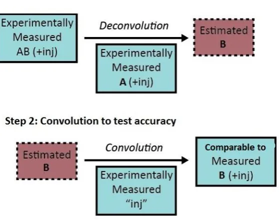
Figure 7: Schematic showing the steps taken in order to assess the accuracy of a single implementation of the deconvolution methods. After deconvoluting measured A from measured AB, the resulting approximation must be convoluted with the measurement of “inj” (at the specific flow rates) in order to be comparable with individually measured B

Figure 8: Experimental tracers as probability distributions for flow 15 ml.min-1 _showing

RTD for: individual volumes A, B; and for the two vessels in series with an extra “inj” volume to aid illustration of experimental error; and for A and B convoluted (which then counts “inj” twice). The comparison of the two AB curves is effectively an indication of experimental error.

3.2.2Comparing model and experimentally measured results

Figure 9: Plots comparing FFT and BAY nitr =100 methods for approximating B from

experimentally measured distributions of AB and A for flowrate 15 ml.min-1_{. (blue dot:}

Table 4: Accuracy of model fit to experimental RTD of B for FFT and BAY nitr =100

Flow rate (ml.min-1₎

MSE x10-8 R2 OVL

FFT BAY FFT BAY FFT BAY

10 1.04 1.04 0.9929 0.9929 0.9461 0.9462

15 5.72 5.72 0.9799 0.9798 0.9146 0.9146

20 7.09 7.08 0.9840 0.9841 0.9148 0.9147

25 2.40 2.40 0.9961 0.9961 0.9554 0.9554

Table 5: Accuracy of model fit to experimental RTD of B for flowrate 10 ml.min-1 _for

FFT and BAY nitr variation with CPU times

MSE x10-8 R2 OVL CPU (s)

BAY nitr =5 3.20 0.9779 0.9268 4.3

BAY nitr =10 1.13 0.9923 0.9415 7.1

BAY nitr =100 1.04 0.9929 0.9462 65

FFT 1.04 0.9929 0.9461 0.4

Essentially the BAY and FFT models produce near identical estimates which are very accurate in all four cases. There is some variation in experimental error, which in all cases is less than the theoretical error introduced in section 3.1.2.

4Conclusions

The three RTD deconvolution models, BAY, LSQ, FFT are all accurate in theoretical tests with no simulated error.

Further tests incorporating simulated error in the convoluted distribution showed that FFT and BAY are very accurate; LSQ is the least suitable.

The polynomial division method is fundamentally unsuitable.

Experimentally tested BAY and FFT models produced near identical results which are very accurate.

R2 and OVL are useful statistical measures here.

BAY does not require any filtering or smoothing here, and so potentially there are applications where it might be practically the most useful, although there may be a runtime penalty.

Acknowledgements

This work was funded through the European Union's Seventh Framework Programme (FP7/2007–2013), grant agreement no. FP7-NMP4-LA-2012-280983, the SHYMAN project. Anonymous advice on a previous draft regarding use of OVL and FFT has been incorporated.

References

Adeosun, J. T. and A. Lawal (2009). "Numerical and experimental mixing studies in a MEMS-based multilaminated/elongational flow micromixer." Sens. Actuators, B 139(2): 637-647. Adschiri, T., Y. Hakuta, K. Sue and K. Arai (2001). "Hydrothermal synthesis of metal oxide nanoparticles at supercritical conditions." J. Nanopart. Res. 3(2-3): 227-235.

Blackburn, J. A. (1970). Spectral analysis: methods and techniques. New York,, M. Dekker. Blood, P. J., J. P. Denyer, B. J. Azzopardi, M. Poliakoff and E. Lester (2004). "A versatile flow visualisation technique for quantifying mixing in a binary system: application to continuous supercritical water hydrothermal synthesis (SWHS)." Chem. Eng. Sci. 59(14): 2853-2861. Boskovic, D. and S. Loebbecke (2008). "Modelling of the residence time distribution in micromixers." Chemical Engineering Journal 135: S138-S146.

Bruce, A. E. R., P. S. T. Sai and K. Krishnaiah (2004). "Characterization of liquid phase mixing in turbulent bed contactor through RTD studies." Chemical Engineering Journal 104(1-3): 19-26.

Cabanas, A., J. A. Darr, E. Lester and M. Poliakoff (2000). "A continuous and clean one-step synthesis of nano-particulate Ce1-xZrxO2 solid solutions in near-critical water." Chemical Communications(11): 901-902.

Clemons, T. E. and E. L. Bradley (2000). "A nonparametric measure of the overlapping coefficient." Computational Statistics & Data Analysis 34(1): 51-61.

Gooseff, M. N., D. A. Benson, M. A. Briggs, M. Weaver, W. Wollheim, B. Peterson and C. S. Hopkinson (2011). "Residence time distributions in surface transient storage zones in streams: Estimation via signal deconvolution." Water Resources Research 47.

Jumbam, D. N., R. A. Skilton, A. J. Parrott, R. A. Bourne and M. Poliakoff (2012). "The Effect of Self-Optimisation Targets on the Methylation of Alcohols Using Dimethyl Carbonate in Supercritical CO2." J. Flow. Chem. 2(1): 24-27.

Krone-Davis, P., F. Watson, M. Los Huertos and K. Starner (2013). "Assessing pesticide reduction in constructed wetlands using a tanks-in-series model within a Bayesian framework." Ecol. Eng. 57: 342-352.

Kuu, W. Y. (1992). "Determination of Residence-Time Distribution in Iv Tubing of in-Line Drug Delivery System Using Deconvolution Technique." International Journal of Pharmaceutics 88(1-3): 369-378.

Langston, P. A. (2002). "Comparison of least-squares method and Bayes' theorem for deconvolution of mixture composition." Chemical Engineering Science 57(13): 2371-2379. Langston, P. A., A. S. Burbidge, T. F. Jones and M. J. H. Simmons (2001). "Particle and droplet size analysis from chord measurements using Bayes' theorem." Powder Technology 116(1): 33-42.

Langston, P. A. and T. F. Jones (2001). "Non-spherical 2-dimensional particle size analysis from chord measurements using Bayes' theorem." Part. Part. Syst. Char. 18(1): 12-21.

Lee, P. M. (2012). Bayesian statistics : an introduction. Chichester, West Sussex ; Hoboken, N.J., Wiley.

Lester, E., G. Aksomaityte, J. Li, S. Gomez, J. Gonzalez-Gonzalez and M. Poliakoff (2012). "Controlled continuous hydrothermal synthesis of cobalt oxide (Co3O4) nanoparticles." Prog. Cryst. Growth Charact. Mater. 58(1): 3-13.

Levenspiel, O. (1999). Chemical reaction engineering. New York, Wiley.

Lucy, L. B. (1974). "Iterative Technique for Rectification of Observed Distributions." Astronomical Journal 79(6): 745-754.

Norby, P., K. M. O. Jensen, N. Lock, M. Christensen and B. B. Iversen (2013). "In situ synchrotron powder X-ray diffraction study of formation and growth of yttrium and ytterbium aluminum garnet nanoparticles in sub- and supercritical water." R. Soc. Chem. Adv. 3(35): 15368-15374.

Particles, P. (2015). "Promethean Particles." from www.prometheanparticles.com.

Richardson, W. H. (1972). "Bayesian-Based Iterative Method of Image Restoration." Journal of the Optical Society of America 62(1): 55-+.

Shyman. (2015). "Shyman." from www.shyman.eu.

Simmons, M. J. H., P. A. Langston and A. S. Burbidge (1999). "Particle and droplet size analysis from chord distributions." Powder Technology 102(1): 75-83.

Viitanen, P. (1997). "Experiences on fast Fourier transform as a deconvolution technique in determination of process equipment residence time distribution." Applied Radiation and Isotopes 48(7): 893-898.