A novel symbolization technique
for time-series outlier detection
Gavin Smith
Horizon Digital Economy Research The University of Nottingham, UK
gavin.smith@nottingham.ac.uk
James Goulding
Horizon Digital Economy Research The University of Nottingham, UK james.goulding@nottingham.ac.uk
Abstract—The detection of outliers in time series data is a core component of many data-mining applications and broadly applied in industrial applications. In large data sets algorithms that are efficient in both time and space are required. One area where speed and storage costs can be reduced is via symbolization as a pre-processing step, additionally opening up the use of an array of discrete algorithms. With this common pre-processing step in mind, this work highlights that (1) existing symbolization approaches are designed to address problems other than outlier detection and are hence sub-optimal and (2) use of off-the-shelf symbolization techniques can therefore lead to significant unnecessary data corruption and potential performance loss when outlier detection is a key aspect of the data mining task at hand. Addressing this a novel symbolization method is motivated specifically targeting the end use application of outlier detection. The method is empirically shown to outperform existing approaches.
Keywords-outlier detection; preprocessing; symbolization; quantization; optimization; time series; data mining
I. INTRODUCTION
Time series are an increasingly prevalent form of mass dataset, due in no small part to the upsurge in human be-havioural data that is now being recorded in an unparalleled fashion in the form of transactional logs. Growing proportions of our daily lives are being logged and recorded, with such data then being leveraged to provide useful insights into a vast array of problems. One important class of such problems is
outlier detection.
Outlier detection within temporal data finds application in a vast range of application areas, with examples including: the detection of changes in the stock market; electronic system diagnostics; biological data analysis; and behavioural pattern analysis [1], [2], [3], [4]. Numerous problem definitions, meth-ods and algorithms have been developed in reference to outlier detection, and the field of uncovering outlying realizations in sets of time series remains an active area of research. However, the pre-processing of time series data is a key step at the heart of many practical implementations of time series analysis. One such pre-processing step is the symbolizationor quantization
of time series: this process describes the mapping of a continu-ous value domain onto an arbitrarily fine discrete domain, thus reducing the complexity of time series representation. Such a technique is routinely employed for a wide variety of reasons, with examples including the addressing of computational
and/or storage constraints (particularly true in data sets of significant size1), noise reduction, interpretation enhancement or to allow the application of algorithms designed specifically for discrete domains [6], [7], [8], [9], [10].
Due in part to the extensive use of symbolization, it is often thought of as a solved problem. However, recently this has been called into question in the general case of time series comparison [11]. That work highlighted two factors: 1. a range of symbolization methods may be characterized by the objective/error function that they seek to minimize; 2. none of the objective functions used by state-of-the-art quantizers were optimal in the broad area of time series comparisons (with that work going on to present an alternative method).
In this paper we evaluate the effectiveness of such quantizers in the area of outlier detection. We similarly note that this is an application area where no optimized strategy currently exists, nor is it clear which of the range of existing techniques available is most effective. Focusing on distance based outlier detection and using a definition for outlier detection that is commonly seen in the context of time series [12], [1]), we reconsider the objective functions of existing symbolization methods and show that they are all suboptimal with respect to the task of outlier detection.
Based on this analysis we then motivate and present an alternative symbolization method tailored specifically for out-lier detection. Finally, we provide an extensive empirical evaluation on four real world datasets, evaluating the proposed approach compared to five existing approaches. In addition to providing a basis of comparison for the proposed approach, this evaluation provides a comparative evaluation as to the utility of existing approaches under such a task (currently only limited comparative evaluation exists). In concluding we highlight the comparative validity of these approaches leading to clear recommendations for practitioners.
II. BACKGROUND
A. Outlier detection via Anomaly Scores
In this work we take an explicit focus on the detection of outlying time series. Given a set of time series, T, we
1For example quantising to 8 symbols can provide a ten or more fold
reduction in storage costs (3 bits per data point vs the typical 32) and the use of symbolized indexing schemes has been shown to enable the indexing of time series numbering into the billions [5]
Published in the Proceedings of the IEEE International Conference on Big Data 2015. c2015 IEEE. Personal use of this material is permitted. Permission from IEEE must be obtained for all other uses, in any current or future media, including reprinting/republishing this material for advertising or promotional purposes, creating new collective works, for resale or redistribution to servers or lists, or reuse of any copyrighted component of this work in other works. IEEE Xplore DOI: http://dx.doi.org/10.1109/BigData.2015.7364037
aim to determine the subset, S ⊂ T, whose elements can be deemed as anomalous. Each individual time series is considered in its entirety2 to be either ‘conforming’ (i.e. following some pre-determined notion of expected behaviour) or ‘nonconforming’. For this task we use the definition of outlying behaviour provided by Chandola et al. [12], whose conception of nonconformity is based upon a time series’
anomaly score, which is defined as follows:
Definition 1: The anomaly score of a data instance is defined as the distance to its kthnearest neighbour in a given dataset.
Armed with this definition the subset of outliers in our dataset can be obtained by specifying an anomaly score threshold, γ and identifying those time series whose scores exceed this threshold. More formally, given a dataset of time series indexed by the natural numbers,T ={T1, T2, . . . , TN},
each individual time series,Ti=hti1, ti2, . . .ican be attributed
an anomaly score, A(Ti|T). These scores allow us to define
the subset of outliers in the dataset as:
S={Ti∈ T |A(Ti|T)≥γ} (1)
A time series anomaly score reflects the distance between itself and it’s kth nearest neighbour. To determine this for
every time series requires an exhaustive series of distance comparisons across the whole dataset - and this reflects a significant computational challenge, especially as the cardi-nality of T increases. Symbolization of time series prior to construction of a distance matrix is hence a popular way of trying to deal with this problem and make processing tractable. However, there is an important issue here - it has been shown that when time series are symbolized, the method selected can have a significant impact on the veracity of time series comparisons [11]. Given the role such comparisons play in anomaly detection, there is therefore also a danger that the choice of the symbolization technique negatively impacts on the veracity of the sets of outliers being identified.
B. Symbolization
As discussed in [11], symbolization can be summarized as a problem of finding an m−level scalar quantizer Q(x). Here Q(x) is a zero-memory nonlinear mapping that takes a real valued scalar input, x, and maps it to one ofm values based on which of the m quantization intervals contains the input. Note that while we focus on a quantizer that is both uni-variate and memory-less, the outcomes of this work are applicable to many extensions such as multivariate quantizers and/or those utilising temporal dependencies [11].
2We note that there also exists a parallel stream of research that considers
the detection of outlying subsequenceswithintime series (as discussed in the recent survey by [1]). While the analysis in this paper could be extrapolated to intra-series anomaly detection, this problem domain is not explicitly considered here.
Formally, ifB0=−∞andBm=∞, then.
(2) Q(x) =
q1 B0< x≤B1
q2 B1< x≤B2
.. .
qm Bm−1< x≤Bm
where the symbolization of a time series Ti = hti1, ti2, . . .i
involves the repeated application of the quantizer to each point in the time series:
ˆ
Q(Ti) =hQ(ti1), Q(ti2), . . .i (3)
The problem of learning a quantizer is then as follows: given some data and an error/objective function, to find the symbol values (i.e. the set of qi values) and boundary values (the
set ofBi values) that minimize that objective function. Thus,
the optimal quantizer is found by solving the optimization problem:
argmin
Q
E(T, Q) (4)
where the error/objective function, E(T, Q), is reflecting the divergence between all of the original time series that ex-ist in our dataset, T and their respective quantized forms,
Q = hQ(Tˆ 1),Q(Tˆ 2), . . . ,Q(Tˆ N)i. The merits of any given
quantizer can only be assessed by how well suited it is to some problem - and consequently how well the objective function used corresponds to the requirements of that problem.
Unlike, say, time series reconstruction, the derivation of a tractable objective function that is optimal foroutlier detection
is a non-trivial task. In such a scenario a desirable function is one that is 1. able to preserve the discriminative information that exists in rare values; and 2. also able to preserve the accuracy of commonly occurring comparisons. If this balance is not correctly established, the value to outlier detection that is gained in emphasising the distances between the rare values (which is, after all, what makes an outlier and outlier), will be lost because of errors that accrue due to neglecting the importance of commonly compared value ranges. Addressing this we motivate and present an adaption of the underlying cost function within the recently proposedICEsymbolization method [11]. Our evaluation of both the method proposed in this work in conjunction with a comparative evaluation of existing techniques highlights a large variance in the relative utility of these approaches with regard to outlier detection, but also demonstrates the superiority of the proposed method.
impact to these of using: time series of different lengths; differing number of symbols being quantized to; and varying parametrisations to the outlier detection algorithm. Finally in
§VI we provide a discussion of the results and conclude with practical recommendations.
C. Existing Symbolization methods
As previously noted, a number of methods for quantizing time series have been proposed in the literature - yet none have specifically addressed the end goal of detecting outlying time series. In this section we provide a concise overview of several prevalent symbolization methods. Each method is motivated by a different purpose, and while some are provably optimal for their original goal none can be considered optimal with respect to detecting outlying behaviour.
1) Uniform quantization (UNI): Uniform quantization is the simplest form of time series quantization, taking into account only therange of values contained in the time series rather than their distributions. A uniform quantizer (UNI) simply splits the value domain into m equal regions, where m is the desired number of symbols. The midpoint of any given region is the new value assigned to any points that fall within its boundaries. Note that while this approach does learn a quantizer Q(x), it does not explicitly optimize an objective function nor consider the distance between the original and symbolized versions of time series.
By not considering the frequency by which symbols occur, UNI favours neither commonly occurring data points (as per MOE, SAX and MSE below) nor commonly compared data points (ICE) at the expense of representing rare data points. In contrast to other methods, however, this agnostic view comes at the expense of over-representation of both unused and unimportant portions of the value domain.
2) Minimal reconstruction error (MSE): Common within the fields of information theory and signal processing, a
minimal reconstruction error quantizer (MSE) [13] seeks to split the value domain into m regions while simultaneously reducing the reconstruction error between the original time series and its symbolized version. If the error is defined as the mean squared distance between each, the objective function in the context of equation 4 can be formulated as:
E(T, Q) = X
Ta∈T
n
X
i=1
(tai−Q(tai))2 (5)
As argued in [11], MSE does not take into account how often comparisons are made between symbols, nor adjust its quantization to optimally maintain pairwisedistancesbetween time series. By only considering time series in isolation, MSE focuses on accurately representing those values that occur frequently. While MSE will in some ways attempt to better model outlying values if their magnitude is large enough, it will still favour a more accurate representation ofcommondata points at the expense of rare values that may provide valuable discriminative information.
3) Maximum Output Entropy (MOE): A Maximum output entropy (MOE) quantizer [14] maximises the average mutual information between the original and symbolized versions of the time series. Maximum entropy occurs when the probability of a value being found in a time series is uniformly distributed - this means that MOE tries to find symbols boundaries that result in a quantized version of the dataset where each symbol occurs an equal number of times. I.e. given each value x occurring in the dataset’s time series, P(B0 < x ≤ B1) =
P(B1< x≤B2)· · ·=P(Bm−1< x≤Bm) = 1/m.
An MOE quantizer hence represents regions of the value domain which exhibit the greatest frequency with more detail, while assigning coarse approximations to regions those that rarely crop up. Similarly to MSE or ICE, an MOE quantizer may therefore plausibly reduce the amount of discriminative information available to detect outliers. Moreover, the concen-trated focus on small but high frequency portions of the value domain may provide no help in trying to preserve the overall distance between two time series. If the large, distinguishing differences between time series are due to the less frequent but more extreme values which exist in the dataset MOE will neglect them - MOE’s focus on information rather than
distancemeans that it may well perform less effectively than quantizers such as MSE and ICE which do take distance into account.
4) Symbolic Aggregation Approximation embedded quan-tizer (qSAX): Symbolic Aggregation Approximation (SAX) is a commonly used symbolic time series representation [15]. SAX and its variants (such as extended SAX [16], iSAX [5], iSAX 2.0 [17]) symbolize not only the value domain, but also the time dimension as well as providing an efficient indexing mechanism. The SAX representation supports any arbitrary underlying quantizer [17, pg. 59], however in this work we compare against the original authors’ [15] choice - an MOE quantizer that assumes a normal distribution over the value domain rather than using the actual empirical distribution of the data (we henceforth denote this approach as qSAX).
5) Independent Comparison Error (ICE): The most re-cently presented symbolization strategy is Independent Com-parison Error (ICE) [11]. ICE considers all possible pairwise comparisons between the time series in the training set. It seeks to minimize, not reconstruction error, but instead the loss in accuracy of the distances between time series. Specifically:
E(T, Q) = X
∀Ta,Tb∈T
|δ(Ta, Tb)−δ( ˆQ(Ta),Q(Tˆ b))| (6)
where δ(Ta, Tb) is the distance between time series Ta
andTb andδ( ˆQ(Ta),Q(Tˆ b))is the distance between the two
quantized time seriesQ(Tˆ a),Q(Tˆ b).
more accurately that pairwise distance will be reflected. This, however, is at the expense of comparisons less often made. Therefore, while initially one may think ICE is ideally suited to outlier detection due to its focus on optimizing comparison fidelity, the deliberate loss of rare discriminative information (which is what tend to identify outliers) in favour of preserving the fidelity of more common comparison makes the overall effectiveness of this approach less clear in this context.
6) Other quantizers: Other quantizers proposed in the literature seek to minimize objective functions specific to their individual problem spaces, utilising additional application specific knowledge. Examples include: perceptual distance quantizers which leverage labelled binary data to symbolize in order to maximise a binary discrimination task [18] and quantizers focusing on maximising quantities such as temporal stability [19] or human perception [20]. Being application specific, unlike the other quantizers detailed, these are not directly applicable to the generalized outlier detection problem considered here.
III. ANOVEL SYMBOLIZATION FOR ANOMALY DETECTION
Notably, the detection of an anomalous time series as de-fined in section II-A is based on pairwise comparisons between time series. As previously noted, however, optimizing compar-ison fidelity directly encourages the representation of common values over rare values, obscuring the discriminative features of any anomalous time series. Acknowledging the need for a better balance between the maintenance of comparison fidelity (to prevent comparison error from common values dwarfing any differences contributed by true anomalous values) and the preservation of rare values, this work presents a modified version of the ICE symbolization approach [11]. Specifically we propose the use of a monotonic transformation function to systematically dampen the error contribution of frequent point-wise symbol comparison pairs within the objective function relative to those compared less frequently.
Such an approach systematically refines the representation of values involved in infrequent comparisons at the expense of a coarser representation of values often compared. The use of a monotonic transformation function ensures that such alterations are relative, with more common values always contributing more error and subsequently obtaining a finer grained representation. As previously discussed, this is desir-able in order to ensure that comparison fidelity in general is maintained and the error introduced from the poor represen-tation of common comparisons does not mask the differences contributed by the rare comparisons that are indicative of anomalous time series.
Specifically, in [11] the objective function of ICE was defined as the measure of the comparison between all time series:
E(T, Q) = X
∀Ta,Tb∈T
|δ(Ta, Tb)−δ( ˆQ(Ta),Q(Tˆ b))| (7)
In order to provide a tractable implementation the distance function, δ(·,·), was set to theL1 norm and the assumption
made that the distance between two time series is well ap-proximated by the sum of the absolute point-wise comparison errors. The resultant objective function was:
(8) ICE(T, Q) =
Z Z ∞
−∞
P(x, y)||x−y|−|Q(x)−Q(y)||dx dy
where P(x, y) denotes the probability of a comparison between valuesx, yover all pairwise time series.
It is this objective function that we extend in this work. Let Γ(·) denote an arbitrary monotonic transformation function. Then the new objective function proposed in this work is:
E(T, Q)= Z Z ∞
−∞
Γ(P(x, y)) RR∞
−∞Γ(P(x, y))
||x−y|−|Q(x)−Q(y)||dx dy
(9)
where the introduced denominator RR−∞∞ Γ(P(x, y)) renor-malizes the probability function after the monotonic transform. In order to adjust the aforementioned trade-off between rarely occurring comparisons and common comparisons such a transform must be a non-constant monotonic transform and reduce the probability of highly probable comparisons to a larger degree than those comparisons with low probability. To this end functions of the form:
Γ(·,·) = (·,·)x1 (10)
are proposed. x acts to control the relative re-weighting of common comparisons probabilities versus infrequent ones. This effectively parametrises the algorithms propensity to provide a finer grained symbolization, and therefore better rep-resent, values that appear infrequently in comparisons versus those that commonly occur. In this work we setx= 2. The resultant objective function, denoted Anomaly Comparison Error (ACE) is:
ACE(T, Q)= Z Z ∞
−∞
p P(x, y) RR∞
−∞
p
P(x, y)||x−y|−|Q(x)−Q(y)||dx dy
(11)
This can implemented as a symbolizer under a framework based upon simulated annealing, and using the same algorith-mic approach asICE3. Such a solution maintains the trivial O(m2) complexity to check a solution within the simulated
annealing (recall that m is the number of output symbols produced by the quantizer, and is assumed to be relatively
3For full details of this algorithmic approach please see [11]. We adapt the
ICE algorithm to allow the efficient implementation ofACEby simply re-placing the use ofP(x, y)in that algorithm with the transformed comparison weighting:
p
P(x, y)
RR∞ −∞
p
P(x, y)
This change modifies the derived function the algorithm uses for pre-computation (denoted asφ(a, b, qij)) in [11]) to:
φACE(a, b, qij) = Z a
−∞
Z b
−∞
p
P(x, y)
RR∞
−∞
p
P(x, y)||x−y| −qij|dx dy
small). As with ICE, a potential bottleneck when computing ACE is in pre-computing the joint probability of comparing any two symbols,P(x, y). However, as noted in [11] this can be alleviated, if required, by accurately approximatingP(x, y) via random sampling of a sufficiently large number of time series4 based on standard statistical techniques.
IV. EMPIRICALEVALUATION
The impact of symbolization on outlier detection tasks has seen limited attention. As such the empirical evaluation has two aims, the first to empirically evaluate the comparative utility of all quantization methods detailed in §II-C and the second to evaluate the novel symbolizer presented in this work. In order to empirically evaluate the comparative utility of the quantization methods with respect to outlier detection as defined in section §II-A we first present an evaluation framework. Recall that:
• the outlier detection problem of interest is the detection of a set of anomalous entities within a large dataset ofNtime series,T =hT1, T2, . . . , TNi.
• the anomaly score of a time series, Ti is defined as the
distance between Ti and itskth nearest neighbour. • an anomalous time series is defined as a time series, Ti
where A(Ti|T) ≥ γ and γ is an application specific
parameter.
Given a fixed number of symbolsm and a quantizer Q(ˆ ·), we define the set of outliers, S, as those items in the dataset that are anomalous, as per equation 1. However, we can form an equivalent set of outliers, Sq, for the quantized version of
the dataset against which to assess performance in the context of outlier detection. One way to do this would be to observe the intersection between S and Sq for a given value of γ.
The higher the intersection of these two sets the better the performance, and if the sets are identical then our quantization has functioned perfectly in the context of outlier detection.
However, if we use the same threshold value for γ in both instances skewed results may occur - γ represents a distance value between two data points and quantization can arbitrarily affect the range over which the pairwise distances are repre-sented. This means that a significantly different number of time series may be identified as outliers in each case. Therefore, it was found preferable to select a different threshold value for the quantized dataset, γq, that ensured the exact same numberof time series,p, were viewed as outliers in both cases. Therefore, if we define:
Sq ={Ti∈ T |A( ˆQ(Ti)|T)≥γq} (12)
where the value for γq is selected such that:
|S|=|Sq|=p (13)
In our experiments we can then vary the value of pto assess the impact of each quantizer over different threshold values, given it is a monotonic function of γ. In practice, since the
4The GPU implementation used can easily compute the joint probability
distribution from tens of thousands of randomly sampled time series.
datasets are of different sizes, we consistently evaluate the definition of an outlier by settingp=β× |T |and vary β.
A. Method
The five quantizers identified in section II-C and the pro-posed approach, ACE, were compared over four real world datasets. Three additional parameters of interest were varied with investigated values are shown in parentheses:
• the number of symbols (m∈ {8,16,24})
• anomaly score definitions (k∈ {1,10})
• outlier definition (β∈ {0.5%,1%,5%,10%)
Each run involved fixingm, k andβ. All of the raw time series were ranked according to their anomaly score for the given value ofk, in order to produce a ground truth based on distance to nearest neighbour.
Rankings were then also produced for symbolized versions of the time series based on the given m value, iterating through each of the quantizers being assessed. Performance of a quantizer could then assessed by: 1. selecting the p = β|T | time series with the highest anomaly scores that it produced; and 2. determining the intersection of that set with theptime series with the highest scores that the ground truth produced. The performance of the quantizer, qPerf, is therefore formally defined as:
qPerf= |S ∩ Sq|
|S| (14)
This statistic may be interpreted as the true positive rate of a binary classifier with a label of outlier being the target class. Reporting other statistics such as the specificity does not provide any additional information since, by definition, each method is restricted to identifying the same number of outliers (with their performance differing only in whichinstancesare identified as outliers).
Within each run the above procedure was repeated15times by redrawing a set of time series randomly from the data set of interest, resulting in15qPerfscores per symbolization method for the given set of parameters. The mean of these15scores was then taken and tabulated indicating the expected perfor-mance of the symbolization method. Pairwise paired t-tests were then conducted between the best performing method and all others, correcting for multiple comparisons via the Holm procedure. Within the tabulated results the best performing method per run is highlighted in bold along with any other method for which no statistically significant difference was observed (p >0.05).
B. Datasets
Smart Meter Electricity data (ELEC): A data set containing over 6435 time series of building energy usage sampled at 30 minute intervals. In total the dataset contains over 400,000 weeks worth of data. The distribution of the combined temporal samples was typically log-normal. Time series lengths of 336 (one week) were considered. The data is from The Commission for Energy Regulation (CER), Electricity Customer Behaviour Trial5. The sampling procedure consisted of randomly selecting an individual and then randomly selecting a week from their data. This procedure was repeated to draw 10,000 time series per sample.
80 Million Tiny Images (IMGS): The second type of real
world data considered was a subset of the 80 Million Tiny Image dataset as detailed in [21]6. Following the work of [17] in evaluating time series, we convert each image to a colour histogram with 256 bins. These histograms can be considered as time series with a length of 256 and the same techniques and evaluation applied. For this experiment a dataset of the first million images was considered. The sampling procedure for this dataset simply consisted of random sampling, with each sample consisting of 10,000 randomly drawn time series.
Retail Transactions (RETAIL): A transactional dataset
from a large UK retailer. The data set consisted of 66,000 individuals, with each individual represented as a time series of with a length of 121, with points within the time series representing consecutive tri-weeks for a period of just over seven years. Each point in the time series corresponded to an individual’s spend for that month. For each sample 4,000 time series were drawn at random from the 66,000 data instances within the set.
Hourly Ozone levels (OZONE): Hourly Ozone levels
recorded at different sites across the US between 2000 and 2015. From the data weekly time series were formed. Only weeks without missing data were kept resulting in 127,085 weeks of data. For each sample 5,000 time series were drawn at random. The data is available via the EPA website7.
V. RESULTS
Results for each of our experimental datasets (ELEC, IMGS, RETAIL and OZONE) are shown in a set of Tables I - IV respectively. The results for each dataset are comprised of six tables (labelled a - f) arranged in a 3x2 grid. Each row shows the results for the dataset when symbolized to either 8, 16 or 24 symbols. The columns distinguish the choice of anomaly score definition used (k). In each individual table the proportion of outliers correctly identified is shown (cell value) for each
5http://www.ucd.ie/issda/data/commissionforenergyregulationcer/ 6Available from http://horatio.cs.nyu.edu/mit/tiny/data/index.html 7http://aqsdr1.epa.gov/aqsweb/aqstmp/airdata/download files.html
0.5% 1% 5% 10%
ACE 0.84 0.89 0.91 0.92
ICE 0.61 0.62 0.79 0.86 qSAX 0.17 0.24 0.47 0.63 UNI 0.64 0.62 0.57 0.60
MSE 0.79 0.82 0.88 0.91
MOE 0.09 0.15 0.36 0.53
(a) Number of Symbols:8,k= 1
0.5% 1% 5% 10%
ACE 0.85 0.87 0.92 0.94
ICE 0.61 0.63 0.77 0.84 qSAX 0.19 0.24 0.47 0.63 UNI 0.69 0.65 0.60 0.63
MSE 0.78 0.82 0.89 0.91
MOE 0.09 0.12 0.35 0.53
(b) Number of Symbols:8,k= 10
0.5% 1% 5% 10%
ACE 0.93 0.93 0.96 0.96
ICE 0.72 0.79 0.91 0.94 qSAX 0.25 0.29 0.56 0.69 UNI 0.79 0.77 0.75 0.76
MSE 0.88 0.91 0.94 0.95
MOE 0.23 0.28 0.55 0.68
(c) Number of Symbols:16,k= 1
0.5% 1% 5% 10%
ACE 0.92 0.93 0.96 0.97
ICE 0.72 0.77 0.89 0.93 qSAX 0.26 0.35 0.58 0.70 UNI 0.83 0.80 0.79 0.79
MSE 0.87 0.90 0.95 0.95
MOE 0.23 0.31 0.57 0.69
(d) Number of Symbols:16,k= 10
0.5% 1% 5% 10%
ACE 0.95 0.96 0.97 0.97
ICE 0.81 0.88 0.94 0.96 qSAX 0.27 0.36 0.60 0.72 UNI 0.87 0.84 0.81 0.81
MSE 0.93 0.94 0.96 0.97
MOE 0.27 0.39 0.62 0.73
(e) Number of Symbols:24,k= 1
0.5% 1% 5% 10%
ACE 0.95 0.96 0.97 0.98
ICE 0.81 0.87 0.93 0.96 qSAX 0.33 0.42 0.61 0.71 UNI 0.88 0.87 0.86 0.85
MSE 0.94 0.93 0.96 0.97
MOE 0.37 0.48 0.63 0.72
(f) Number of Symbols:24,k= 10
TABLE I: Results: RETAIL. Time series length: 121. Bold: best performing (statistically inseparable, p > 0.05) method(s).
symbolization method (rows) as the outlier definition (β) is varied.
Across all methods results show a minimal impact of varying k, and expected increases in performance as β and the number of symbols are increased. Between the methods themselves the results indicate the proposed approach in general out-performs or equals all other methods (in 76% of cases) or is within a relatively small error margin (<5% in 20.8.% of cases, ≥ 5% in 3.1% of cases). In contrast, the next two best performing methods, MSE and UNI, achieved the highest or equal highest score only 38.5% and 30.2% of the time respectively. Notably when under-performing the approaches did so with a greater margin. Specifically MSE under-performed by a error margin ≥ 5% in 28.1% of the cases. UNI perform worse again under-performing by a error margin ≥ 5% in 42.7% of the cases. Of the remaining methods, ICE performed significantly better on average than MOE and SAX but compared to ACE showed mediocre performance.
VI. DISCUSSION
A. Top performers: ACE, MSE and UNI
0.5% 1% 5% 10%
ACE 0.93 0.92 0.92 0.90
ICE 0.70 0.79 0.93 0.94
qSAX 0.11 0.16 0.53 0.73 UNI 0.84 0.81 0.86 0.73
MSE 0.89 0.91 0.94 0.93
MOE 0.05 0.05 0.24 0.50
(a) Number of Symbols:8,k= 1
0.5% 1% 5% 10%
ACE 0.97 0.95 0.95 0.93
ICE 0.70 0.88 0.96 0.95
qSAX 0.09 0.14 0.53 0.76 UNI 0.91 0.88 0.92 0.76
MSE 0.95 0.95 0.97 0.95
MOE 0.04 0.05 0.23 0.49
(b) Number of Symbols:8,k= 10
0.5% 1% 5% 10%
ACE 0.97 0.97 0.97 0.96
ICE 0.90 0.92 0.97 0.97
qSAX 0.15 0.24 0.65 0.81 UNI 0.94 0.92 0.89 0.88
MSE 0.96 0.97 0.97 0.97
MOE 0.10 0.15 0.49 0.71
(c) Number of Symbols:16,k= 1
0.5% 1% 5% 10%
ACE 0.98 0.98 0.98 0.97
ICE 0.92 0.96 0.98 0.98
qSAX 0.11 0.19 0.67 0.84 UNI 0.97 0.95 0.93 0.91
MSE 0.98 0.98 0.99 0.98
MOE 0.08 0.12 0.49 0.73
(d) Number of Symbols:16,k= 10
0.5% 1% 5% 10%
ACE 0.99 0.99 0.98 0.97
ICE 0.96 0.96 0.98 0.98
qSAX 0.17 0.28 0.71 0.84 UNI 0.96 0.96 0.91 0.89
MSE 0.98 0.98 0.98 0.98
MOE 0.14 0.23 0.64 0.80
(e) Number of Symbols:24,k= 1
0.5% 1% 5% 10%
ACE 0.99 0.99 0.99 0.98
ICE 0.96 0.98 0.99 0.98
qSAX 0.13 0.21 0.73 0.86 UNI 0.98 0.97 0.93 0.91
MSE 0.99 0.99 0.99 0.99
MOE 0.10 0.18 0.66 0.83
[image:7.612.50.570.61.281.2](f) Number of Symbols:24,k= 10
TABLE II: Results: ELEC. Time series length: 336. Bold: best performing (statistically inseparable,p >0.05) method(s).
0.5% 1% 5% 10%
ACE 0.86 0.82 0.72 0.68
ICE 0.63 0.58 0.72 0.76 qSAX 0.02 0.06 0.28 0.39 UNI 0.78 0.73 0.28 0.21
MSE 0.81 0.80 0.79 0.79
MOE 0.01 0.02 0.09 0.15
(a) Number of Symbols:8,k= 1
0.5% 1% 5% 10%
ACE 0.80 0.84 0.80 0.75
ICE 0.60 0.66 0.70 0.76 qSAX 0.00 0.01 0.19 0.31 UNI 0.76 0.84 0.55 0.36
MSE 0.72 0.79 0.81 0.83
MOE 0.00 0.01 0.06 0.12
(b) Number of Symbols:8,k= 10
0.5% 1% 5% 10%
ACE 0.93 0.92 0.88 0.85
ICE 0.75 0.82 0.84 0.84 qSAX 0.02 0.09 0.36 0.48 UNI 0.86 0.80 0.71 0.49
MSE 0.88 0.90 0.89 0.88
MOE 0.01 0.03 0.17 0.25
(c) Number of Symbols:16,k= 1
0.5% 1% 5% 10%
ACE 0.89 0.91 0.93 0.91
ICE 0.72 0.73 0.83 0.85 qSAX 0.00 0.02 0.24 0.40 UNI 0.91 0.89 0.81 0.74
MSE 0.86 0.89 0.92 0.92
MOE 0.00 0.01 0.11 0.20
(d) Number of Symbols:16,k= 10
0.5% 1% 5% 10%
ACE 0.95 0.95 0.92 0.90
ICE 0.88 0.89 0.90 0.91 qSAX 0.04 0.10 0.39 0.51 UNI 0.91 0.87 0.74 0.72
MSE 0.92 0.93 0.92 0.92
MOE 0.01 0.05 0.24 0.33
(e) Number of Symbols:24,k= 1
0.5% 1% 5% 10%
ACE 0.93 0.95 0.95 0.95
ICE 0.79 0.83 0.90 0.92 qSAX 0.00 0.03 0.27 0.43 UNI 0.94 0.93 0.83 0.81
MSE 0.91 0.92 0.95 0.94
MOE 0.00 0.01 0.16 0.26
(f) Number of Symbols:24,k= 10
TABLE III: Results: IMGS. Time series length: 336. Bold: best performing (statistically inseparable,p >0.05) method(s).
was significantly more consistent in its performance compared to its closest competitors, UNI and MSE over the datasets investigated.
Between MSE and UNI, MSE performed better than UNI except within the OZONE dataset. While the values com-prising the time series within all datasets have a distribution somewhat positively skewed, compared to the other dataset the distribution of values in the OZONE dataset is more evenly distributed. As such since there are more common
values. In such a case, by minimizing the reconstruction error
0.5% 1% 5% 10%
ACE 0.80 0.81 0.85 0.85
ICE 0.25 0.34 0.60 0.71 qSAX 0.13 0.23 0.48 0.62 UNI 0.82 0.78 0.75 0.73
MSE 0.46 0.53 0.70 0.76
MOE 0.15 0.22 0.48 0.62
(a) Number of Symbols:8,k= 1
0.5% 1% 5% 10%
ACE 0.82 0.85 0.88 0.88
ICE 0.24 0.32 0.58 0.70 qSAX 0.13 0.19 0.46 0.60 UNI 0.86 0.85 0.81 0.81
MSE 0.50 0.55 0.73 0.79
MOE 0.12 0.19 0.46 0.59
(b) Number of Symbols:8,k= 10
0.5% 1% 5% 10%
ACE 0.89 0.89 0.91 0.91
ICE 0.54 0.62 0.79 0.86 qSAX 0.28 0.37 0.62 0.75 UNI 0.93 0.91 0.90 0.89
MSE 0.83 0.83 0.86 0.87
MOE 0.29 0.38 0.63 0.75
(c) Number of Symbols:16,k= 1
0.5% 1% 5% 10%
ACE 0.90 0.91 0.93 0.93
ICE 0.54 0.60 0.80 0.87 qSAX 0.25 0.33 0.61 0.74 UNI 0.94 0.95 0.93 0.93
MSE 0.85 0.85 0.88 0.89
MOE 0.26 0.34 0.61 0.74
(d) Number of Symbols:16,k= 10
0.5% 1% 5% 10%
ACE 0.91 0.93 0.93 0.93
ICE 0.88 0.88 0.91 0.92
qSAX 0.37 0.45 0.69 0.81 UNI 0.95 0.95 0.93 0.93
MSE 0.89 0.90 0.90 0.90
MOE 0.37 0.46 0.70 0.82
(e) Number of Symbols:24,k= 1
0.5% 1% 5% 10%
ACE 0.92 0.94 0.94 0.94
ICE 0.89 0.89 0.92 0.94 qSAX 0.33 0.41 0.68 0.80 UNI 0.95 0.97 0.95 0.96
MSE 0.89 0.92 0.92 0.93
MOE 0.34 0.43 0.70 0.81
[image:7.612.52.301.331.550.2](f) Number of Symbols:24,k= 10
TABLE IV: Results: OZONE. Time series length: 168. Bold: best performing (statistically inseparable, p > 0.05) method(s).
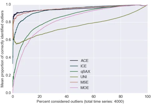
MSE systematically under-represents the rare discriminating values to a greater degree in order to better represent the larger number of common ones. In contrast, UNI uses a fixed resolution across the value domain maintaining a relatively finer grained resolution for the rare values compared to MSE for the OZONE dataset. However, in other datasets this is a significant drawback. By not allocating more symbols at a finer resolution for commonly occurring values, more subtle but more frequently occurring differences are removed with the error generated quickly dwarfing the correctly measured difference due to the more accurately represented rare values. The lack of adaption to the data in UNI also presents itself as an issue for concern as the definition of an outlier is relaxed. Across all symbolization methods results generally exhibit the intuitive behaviour of increased performance as the definition of an outlier is relaxed (increase in β). Notably, however, such performance does not hold for the UNI method, with performance observed to decreasein Table III (a) and (b) as β increased from 1−10%. While perhaps not immediately obvious such behaviour is understandable. Note that the ex-pectation for an increase in performance asβincreases comes from the split between outliers and non-outliers being based on separating off a largeroutliers group, which will typically be based on more and more common differences (values) which the majority of symbolization strategies are designed towards. However, this is not the case for UNI and as such the expectation for improvement with increasedβ is unfounded.
Fig. 1: RETAIL dataset, k = 1, m = 8. β varied over all possible parameters up to the degenerate case where all data is considered outliers (β = 100%). Note that only the very left most part of the graph would be considered as representing outlier detection under typically definitions.
exhibit increased performance as the definition of an outlier is relaxed with the exception of UNI. The results lend further evidence against the use of the UNI symbolization approach. Similar figures were plotted for the other datasets with similar results which are omitted due to space constraints.
B. Average performance of ICE
While sharing a similar theoretic underpinning to ACE, ICE performed significantly worse, under-performing to both MSE and UNI as well as ACE. While one might expect ICE to perform better due to the focus on maximising an objective function based on comparisons (which plays a large role under the definition of an outlier considered in this work), the results empirically demonstrates the previously discussed side effect of such an optimization - that optimizing comparison fidelity directly encourages the representation of common values over rare values. Since rare values are required to distinguish outliers, this re-enforces the argument that there is no one optimal symbolization strategy.
C. Weak performance of MOE and qSAX
Overall, MOE and qSAX consistently performed the worst. The poor performance of MOE and qSAX is perhaps not unsurprising. As noted in section II-C, the optimization of the MOE representation only takes into account the resultant symbol counts. As such MOE favours the representation of common values over rare ones without any consideration for the significant loss of information that would bring in
distinguishing a time series from all the other in the original value domain. Based on the same underlying principle but assuming a normal distribution of the time series’ values, qSAX’s similarly poor performance is also not unexpected. Clearly that the closer the data distribution is to being normal the more the method will inhered the drawbacks present in
MOE. Note, however, if the assumption of normality is not satisfied it does not mean that one would expect qSAX to perform well as it would be random chance whether the important areas of the value domain were well represented (represented with high detail) or not.
VII. CONCLUSION
Embedded in many applications of outlier detection, sym-bolization is a common form of pre-processing in time series data, enabling less computational resources to be used and enabling the application of discrete algorithms. Taking the often used definition of an outlier as one with an unusually large distance to any other data instances we note that while numerous symbolization techniques have been proposed none are guaranteed to be optimal within this problem domain. Noting this, a non-trivial symbolization approach directly considering the application of outlier detection was proposed. Additionally providing an analysis of the relative and absolute performance of existing methods for which performance is non-obvious, an set empirical experiments was undertaken on four real world datasets. The empirical results show the superi-ority of the proposed approach and highlight a stark difference in the resultant ability to correctly determine outliers between different methods. Such results highlight the significant impact the choice of quantizer makes in real world applications.
The results suggest that the proposed approach, ACE, is able to consistently achieve a higher accuracy in identifying time series outliers than other methods using less resources (number of symbols) and therefore should be preferred in the general case. Depending on the dataset MSE or UNI may be appropriate, however, the wrong choice can have significant practical implications degrading performance by over 30% compared to ACE (e.g. MSE: Table IV (a), UNI: Table I (b)). In clear second place was the minimum reconstruction error (MSE) quantizer. Results indicate that while a uniform symbolization may be tempting due to its simplicity it should be avoided with the approach showing a drop of at least 5% accuracy in nearly half the parameterizations examined. Often, however, this was much greater, up to47%. Finally, while not surprising, we note that the quantizer within the often used SAX time series representation (or subsequent iSAX, or iSAX 2.0 representations) should not be used, with the approach significantly under-performing to ACE, MSE or UNI over all datasets and parameterizations. This should not deter the use of such representation, but if such representations are used then the quantizer within these representations should be replaced with a more suitable quantizer such as ACE.
VIII. ACKNOWLEDGMENTS
This work was jointly supported by the EPSRC
REFERENCES
[1] M. Gupta, J. Gao, C. Aggarwal, and J. Han, “Outlier detection for temporal data: A survey,” Knowledge and Data Engineering, IEEE Transactions on, vol. 26, no. 9, pp. 2250–2267, Sept 2014.
[2] M. Gupta, J. Gao, Y. Sun, and J. Han, “Community trend outlier detection using soft temporal pattern mining,” inMachine Learning and Knowledge Discovery in Databases. Springer, 2012, pp. 692–708. [3] S. A. Hofmeyr, S. Forrest, and A. Somayaji, “Intrusion detection
using sequences of system calls,” J. Comput. Secur., vol. 6, no. 3, pp. 151–180, Aug. 1998. [Online]. Available: http://dl.acm.org/citation. cfm?id=1298081.1298084
[4] P. Sun, S. Chawla, and B. Arunasalam, “Mining for outliers in sequential databases.” inSDM. SIAM, 2006, pp. 94–105.
[5] J. Shieh and E. Keogh, “iSAX: disk-aware mining and indexing of massive time series datasets,”Data Mining and Knowledge Discovery, vol. 19, no. 1, pp. 24–57, 2009.
[6] V. Chandola, A. Banerjee, and V. Kumar, “Anomaly detection for discrete sequences: A survey,”Knowledge and Data Engineering, IEEE Transactions on, vol. 24, no. 5, pp. 823–839, May 2012.
[7] S. Das, B. L. Matthews, A. N. Srivastava, and N. C. Oza, “Multiple kernel learning for heterogeneous anomaly detection: Algorithm and aviation safety case study,” inProc. 16th ACM SIGKDD Intl. Conf. on Knowledge Discovery and Data Mining, ser. KDD ’10. New York, NY, USA: ACM, 2010, pp. 47–56.
[8] B. Hu, T. Rakthanmanon, Y. Hao, S. Evans, S. Lonardi, and E. Keogh, “Discovering the intrinsic cardinality and dimensionality of time series using MDL,” inProc. Int’l Conf. Data Mining, 2011, pp. 1086–1091. [9] E. Keogh, J. Lin, and A. Fu, “Hot sax: Efficiently finding the
most unusual time series subsequence,” in Proceedings of the Fifth IEEE International Conference on Data Mining, ser. ICDM ’05. Washington, DC, USA: IEEE Computer Society, 2005, pp. 226–233. [Online]. Available: http://dx.doi.org/10.1109/ICDM.2005.79
[10] G. Smith, R. Wieser, J. Goulding, and D. Barrack, “A refined limit on the predictability of human mobility,” inPervasive Computing and Communications (PerCom), 2014 IEEE Intl. Conf. on, March 2014, pp. 88–94.
[11] G. Smith, J. Goulding, and D. Barrack, “Towards optimal symbolization for time series comparisons,” in Data Mining Workshops (ICDMW), 2013 IEEE 13th Intl Conf on. IEEE, 2013, pp. 646–653.
[12] V. Chandola, A. Banerjee, and V. Kumar, “Anomaly detection: A survey,” ACM Computing Surveys (CSUR), vol. 41, no. 3, p. 15, 2009. [13] J. Max, “Quantizing for minimum distortion,”Information Theory, IRE
Transactions on, vol. 6, no. 1, pp. 7–12, March 1960.
[14] D. Messerschmitt, “Quantizing for maximum output entropy (corresp.),” Information Theory, IEEE Transactions on, vol. 17, no. 5, pp. 612–612, 1971.
[15] J. Lin, E. Keogh, S. Lonardi, and B. Chiu, “A symbolic representation of time series, with implications for streaming algorithms,” inProc. SIGMOD Workshop on Research Issues on Data Mining and Knowledge Discovery (DMKD). ACM, 2003, pp. 2–11.
[16] B. Lkhagva, Y. Suzuki, and K. Kawagoe, “Extended SAX: Extension of symbolic aggregate approximation for financial time series data representation,” inProc. Int’l Conf. Data Mining Workshops, 2006. [17] A. Camerra, T. Palpanas, J. Shieh, and E. Keogh, “iSAX 2.0: Indexing
and mining one billion time series,” inProc. Int’l Conf. Data Mining (ICDM). IEEE, 2010, pp. 58–67.
[18] H. Poor and J. Thomas, “Applications of ali-silvey distance measures in the design of generalized quantizers,”IEEE Trans. Communications, vol. 25, no. 9, pp. 893–900, 1977.
[19] F. M¨orchen and A. Ultsch, “Optimizing time series discretization for knowledge discovery,” inProc. Int’l Conf. Knowledge discovery in data mining (KDD). ACM, 2005, pp. 660–665.
[20] C. Mota and J. Gomes, “Optimal image quantization, perception and the median cut algorithm,”Anais da Academia Brasileira de Ciłncias, vol. 73, pp. 303 – 317, Sept. 2001.