Development Of Methods For Optimisation Of Complex 3D
Weave Geometries
G H Spackman1, L P Brown1 and I A Jones1
1 Composites Research Group, Faculty of Engineering, University of Nottingham, Nottingham, United Kingdom
Corresponding Author: [email protected]
Abstract. The development of 3D weaves has resulted in the ability to produce near net shaped preforms, with the additional advantage over unidirectional lay-ups and 2D weaves of greater delamination resistance provided by through-thickness reinforcement. 3D weaving can allow the post-weave formation of bifurcations to form the web and flange of structural components. The mechanical properties of 3D woven components are highly dependent on the weave architecture, allowing the mechanical performance of the component to be tailored to its specific application. Given the number of design parameters to be varied, the design space is potentially infinite. This work focuses on the development of methods to find the optimum weave geometry of a unit cell based on the numerical evaluation of objective functions.
This work demonstrates the development of methods to optimise 3D woven textile geometry, using the University of Nottingham’s open-source software TexGen [1] to automatically generate each weave based on the input from a global optimisation algorithm. Methods of varying a number of the parameters will be reported alongside their geometric and physical constraints. Finally, the facility to automatically generate a wide range of weaves, with the ability to vary parameters as desired for input either directly into an optimisation algorithm or for further pre-processing is demonstrated.
1. Introduction
T and I joint beams are typically used in the aerospace industry as skin stiffeners, spar to skin joints and bulkhead joints. Typical in-service loading conditions include tensile and flexural loads [2–4]. These present conventional composite laminates with the problem of increased risk of delamination between the plies. It has been shown that composite 3D weaves have the advantage over laminates of greater through the thickness reinforcement which leads to greater impact resistance [5] and delamination properties [6]. Reduced fibre damage and crimp during the manufacturing process is an additional advantage of 3D weaving over z-pinning and stitching methods.
Due to material anisotropy, the mechanical performance of 3D woven structures is highly dependent on the meso-scale fibre architecture, allowing each structure to be tailored directly to its specific application. Some parameters that can be varied include the number of layers, the path of the reinforcing z-binders and the yarn cross-sections.
main algorithm employed in the field is the so-called ‘genetic algorithm’ which is known for its robustness, availability and ease of use as it has been implemented as an ‘out of the box’ function in MATLAB [7]. However, there is little information regarding its efficacy in comparison to other direct search algorithms.
An optimisation framework has been developed in [7, 8] to find optimum 3D weave architectures of flat woven pieces by obtaining the material moduli. Later in [10] Yan simulated several weave configurations by varying the weft yarn path of a woven T-joint in a tensile pull-off test, creating the weave variations manually. The aim of this work is to adapt the optimisation framework implemented to optimise the flat pieces and apply it to automatically generated FE models of T-pieces, replicating the tensile pull off test in Yan’s work while being able to constrain the textile binder yarn paths to the feasible domain.
The use of optimisation algorithms relies on the ability to automatically generate a large number high fidelity finite element models with complex weave variations by creating a parameterised weave and then varying those parameters. The University of Nottingham’s in-house geometric modelling software TexGen [1], can be used as a pre-processor for a finite element package, such as the commercial solver Abaqus, by creating the textile geometry and then automatically meshing with a voxel mesh before exporting to Abaqus for analysis under the specified loading conditions.
This study develops previous work by applying it to complex shape profiles with finite element simulations not limited to finding elastic moduli in unit cells. Following this, methods to find the optimum reinforcement architecture of a reduced model of the woven T-joint structure will be presented. Optimisation was by genetic algorithm for initial stiffness under an out of plane tensile load through the web of the joint. The developments in the optimisation framework will be presented along with a demonstration of a constraint handling method.
The novel aspects of this study include the application of the current optimisation framework to a post-deformation, idealised 3D model with a more complex objective function and the novel constraint handling algorithm.
2. Optimisation Problem and Constraints An optimisation problem is defined as:
minimise objective function f(x), subject to constraints gi(x) ≤ 0
and hi(x)=0
within bounds xL≤ x ≤xU (1)
where x is a vector of the design variables in the optimisation problem, gi(x) are the inequality constraints
and the hi(x) are the equality constraint functions. The constraint functions are handled differently
depending on whether they are linear or nonlinear. If there is constraint violation then a penalisation factor may be added to prevent the solution being considered as the minimum.
In this work the objective function is the initial stiffness of a reduced T-joint under tensile loading through the flange, a typical in service loading condition for this type of component. The T-joint is woven using crimp free yarns and the objective function is evaluated using the commercial finite element software, Abaqus [11]. In this case the path of the binder yarns at the junction were varied. This simple objective function was chosen to be able to demonstrate the ability of the optimisation framework to be applied to complex 3D woven structures. The genetic algorithm was used due to its ease of implementation.
1. One binder must pass over the top and another must pass under the bottom of each weft stack to ensure all the weft yarns are bound.
2. No straight, non-reinforcing binder yarns above or below weft stacks.
3. At least one binder yarn must cross all horizontal planes between weft layers in the unit cell to prevent separation of the textile.
The second constraint is easily implemented with a simple linear constraint. This, along with bounds, defines the region of feasible design solutions with respect to the linear constraints. In the genetic algorithm optimisation framework, MATLAB only generates feasible members with respect to the linear constraints, so the second constraint is automatically satisfied for each iteration.
Constraints 1 and 3 are difficult to write down in equation form, therefore, a novel algorithm was developed based on the binder yarn offsets from the top of the textile to determine whether or not a weave violates the constraints. This algorithm is used to add a penalty factor, post FE analysis, if constraint violation is found. This raises the effective objective function value and makes it unlikely that the optimisation algorithm will find that solution to be a minimum of the function f(x).
The objective function is calculated via finite element simulations, the load – displacement curve is plotted from the extracted data and the initial gradient calculated.
3. Optimisation Algorithms
The use of optimisation algorithms for finding the optimum composite design is well documented in the literature for laminates, with the genetic algorithm often chosen as the solver of choice [11-14]. Frequently, little justification is given for the choice of algorithm with the choice in practice often made on the basis of peer advice and/or prior familiarity.
3.1 Genetic Algorithm
The genetic algorithm is a population based solver based on the Darwinian principle of survival of the fittest. There are four stages:
1. Initialisation - An initial population of member solutions is generated with the set of design variables analogous to the genotype of that member. The linear constraints and bounds are satisfied here.
2. Selection - Each member solution is evaluated and given a fitness value. A penalty may be applied here if the member violates the nonlinear constraints. The population is then ranked with the best performing or elite solutions entered directly into the next generation.
3. Mutation - Of the remaining solutions, some of their design variables undergo a small alteration creating a slightly different combination of design variables which are then entered into the next generation. Analogous to gene mutations in biology.
4. Crossover - Two well performing textiles have their design variables combined to produce a new set of design variables. This process is analogous to breeding amongst a population. The rest of the next generation is made up of new initialised members.
By continuing this process, the optimum solution should be found that satisfies all the linear and nonlinear constraints.
4. Optimisation of a T-Joint
T-joint, the as woven geometry was modelled first in TexGen before the geometric transformations set out in [10] were employed to fold out the bifurcated part into the shape of a T. The model is then automatically meshed with voxel elements and submitted for finite element analysis in Abaqus. Post-analysis the binder yarn configuration is checked using a novel algorithm with a penalty factor added based on the constraint violation.
4.1 Optimisation Framework
The optimisation process is controlled via an algorithm implemented in Matlab which writes the design variables, in this case the binder yarn offsets, to a text file. Matlab then launches Abaqus and runs using its Python interface a script that uses the TexGen functions to set up the geometrical model, mesh it and apply the loads and boundary conditions before submitting the job for analysis. Once the job is finished, the objective function value is calculated from the extracted data and the penalty function added in the same Python script. The final value is written to a second text file from which Matlab reads in the final value. This process is repeated every time the algorithm produces a new set of design variables and continues until the algorithm’s convergence criteria are met.
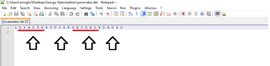
[image:4.595.71.525.418.530.2]4.1.1 Varying Binder Yarns. To vary the binder yarn offsets and create different binder paths, the main Python script read in the final data line from the text file. Each data point in the data file is an offset from the top of the textile. For example, to define a binder yarn path in a textile with 6 weft yarns requires a data point each. Therefore, with 4 yarns there were 24 offset data points on each line of the data file, see figure 1. The TexGen function SetBinderPosition was then used to set the binder offset position.
Figure 1. Data file containing the design variables for use in genetic algorithm optimisation. Each arrow points to the data points that define a single yarn in a textile with 6 weft stacks.
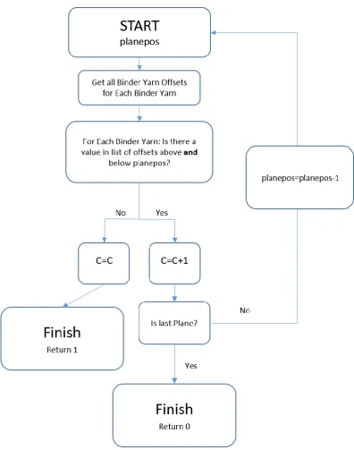
4.1.2 Penalty Algorithm. In order to ensure the optimum textile produced using the algorithm conforms to the constraints on the binder yarns set out in section 2, checking methods were developed to determine constraint violation for constraints 1 and 3.
The function to check constraint 1, that a binder must pass above and below each weft stack, takes all the binder offsets and orders them into lists; each list contains all the offsets in a weft stack. It then checks whether there is an offset value of 0,indicating a binder passing over the stack, and whether there is an offset value equal to the number of layers, implying a binder passing underneath the stack. If one or both of these are not present in the list a penalty is added. This process is repeated for each weft stack.
Figure 2. Flow chart of algorithm to implement constraint 3.
where planepos is the plane position of an internal plane.
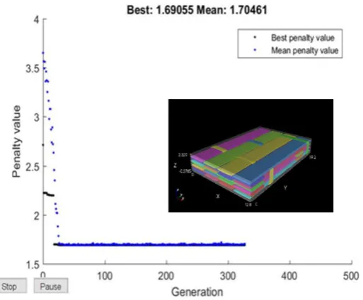
Figure 3. Graph of Penalty Value against Generation for optimisation showing the effect of the penalty parameter alongside the TexGen model of the optimum weave.
The textile produced conformed to all the constraints within around 20 generations. It can be seen that once the feasible domain has been reached, further variations in the weaving pattern causes little variation in the penalty value. This demonstrates the effectiveness of the constraint handling algorithm in forcing the genetic algorithm into the feasible domain.
4.2 Flat Woven Parameterised Weave
The T-joint is woven flat with the binder yarns constrained in different halves of the textile, binding only half the weft stack. This allows the creation of the bifurcation post weaving. The as-woven geometry is created as a parameterised weave using TexGen’s CTextileLayerToLayer class with the parameters in Table 1.
Table 1. List of parameters used to create the as-woven flat model with 4 binder yarns
Parameters of CTextileLayerToLayer Class
Number of X Yarns Number Y Yarns
X Spacing Y Spacing Warp Height
Weft Height Number of Binder Layers
10 6 3.2 3.2 0.35 0.25 1
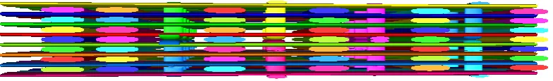
[image:6.595.151.443.568.706.2]the noodle or junction area, a simplification was made so that the binder yarns have to stay in the top half of the structure and were then copied and transformed to bind the lower half of the structure. This results in a textile that separates into two layers, see figure 4.
Figure 4. The flat as-woven geometry showing the binder yarns constrained in separate layers.
4.3 Bifurcated Model
Once the flat geometry has been created, a geometric transformation is applied to both the nodes and the yarn cross-sections, as set out by Yan in [10] and listed in equation 2. This creates the profile shape of the T and models the effect of the mould in the creation of the bifurcation. The angle the yarns make from a specified origin can be characterised by the position along the length of the weft yarn by the angle 𝛽 as below.
𝛽 = {
𝑦′ 𝑧′ 𝑓𝑜𝑟
𝜋 2𝑧
′≥ 𝑦′ > 0
𝜋
2 𝑓𝑜𝑟 𝑦
′ >𝜋 2𝑧
′ (2)
This is used to determine which of the transformations in equation (2) to apply depending on the position of the node along the undeformed yarn.
∆𝑦 = {𝑧
′sin 𝛽 − 𝑦′ 𝑓𝑜𝑟 𝜋
2𝑧
′≥ 𝑦′ > 0
𝑧′− 𝑦′ 𝑓𝑜𝑟 𝑦′>𝜋
2𝑧
′ (3)
and
∆𝑧 = { 𝑧
′cos 𝛽 − 𝑧′ 𝑓𝑜𝑟 𝜋
2𝑧
′≥ 𝑦′ > 0
(𝜋2𝑧′− 𝑦′) − 𝑧′ 𝑓𝑜𝑟 𝑦′ >𝜋2𝑧′ (4)
Figure 5. Bifurcated Model
4.4 Meshing
One of the main difficulties in the optimisation of weaving patterns is the automatic generation of a mesh, needed to allow the optimisation process to run without user interaction. It is difficult to mesh contacting yarns using conformal meshing. The solution is to employ voxel meshing [10] which involves the use of brick shaped hexahedral elements which are tessellated throughout the geometrical volume in a method analogous to the use of pixels in imaging.
Each voxel element is defined by its centre point and orientation. The voxel is assigned to be either matrix or yarn depending on which region its centre point lies within. In general, this method of meshing results in a jagged interface boundary which can lead to a greater interface stiffness or interlocking of the elements at the boundaries depending on the local stress condition [10]. However, the interface stiffness can be scaled following the procedures set out in the referenced work.
TexGen automatically meshes within a specified volume or domain set up by the user, either by assigning a default domain normally representing the unit cell or by specifying domain planes that enclose the volume. Currently, these domain planes must form a convex. For a complex shape with concave parts such as a T-joint the smallest shape that will enclose the T-joint is a cuboid.
When the model is meshed and exported using an Abaqus .inp file, the parts of the domain that are enclosed within the yarns are meshed with elements defined with the yarn properties while the rest of the domain is assigned the properties of the matrix. When the T-joint is meshed and exported, the result is a cuboid with surplus matrix elements with the yarn elements, forming the T-shape, embedded within. To represent the shape of the final composite component the extra matrix elements and nodes were deleted in Abaqus’ part module using Python scripting. Once this was done the finite element model was set up.
4.5 Finite Element Model
The finite element model needs to be able to be automatically generated and submitted in Abaqus each time a new weave is created by the optimisation algorithm. The aim is to be able to create an accurate enough model each time while taking account of the computational expense of a large number of finite element simulations.
4.5.1 Modelling the Tensile Pull Off Test
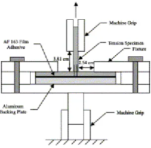
the gradient. In experimental and numerical simulations of the tensile pull out test, Yan found that the load-displacement curve rises linearly until a peak load is reached at a displacement of around 1mm where material damage has initiated and there is a drop in stiffness. Material damage comes mainly in the form of delamination and matrix cracking. The curve then rises further as the damaged component can still sustain a large load before catastrophic failure occurs between 5-7mm depending on the weaving pattern. A simplified diagram of the test is shown in Figure 6.
Figure 6. Diagram of the tensile pull off test, taken from [4].
Due to the large size of the model and the small element size needed to capture the geometry
accurately, a reduced model focussing on the junction area was employed. This is an attempt to reduce the time and computational expense which finite element simulations of the full model would require. In addition to focussing closely on a smaller area of interest, the initial stiffness was chosen as the objective function.
In order to model the test, a displacement controlled loading scheme is applied in Abaqus to the nodes along the top surface of the web. The load is increased in a displacement controlled manner until the 1mm mark is reached. To model the clamping of the flange, encastre boundary conditions were applied to the bottom corners of the model. This would allow normal rotation of the noodle area while restricting rigid body motion, Shown in Figure 7.
[image:9.595.202.437.536.735.2]The mesh was made up of 421,875 Abaqus C3D8R voxel elements, this mesh density was chosen as it best captured the yarn geometry which can include many gaps where it is difficult to distinguish between yarns and matrix if the mesh size is too large.
Once the model was set up and meshed and the loads applied, the models were submitted for analysis. The whole process of model set up and submission is automated using a Python script, following the process set out in previous optimisation work.
5. Discussion
Automatically meshing shapes with complex profiles such as the T-shape is currently difficult. TexGen generates the voxel mesh elements by dividing up a volume containing the model called the domain. The domain is specified by a set of planes. However, currently only domains that are convex in shape are able to be defined. This is due to the multiple plane intersections that would occur in concave shapes such as T-profiles, making it difficult to determine which intersection is required to form the domain. This works well for the vast majority of cases where unit cells are used to apply periodic boundary conditions as the woven cell is typically cuboidal in shape. However, for complex shapes this provides a significant barrier to automatic mesh generation. In previous work by Yan [16] the voxel mesh was automatically generated for a cuboid containing the embedded T-profile. This leads to an excess of matrix elements which Yan removed manually using the HyperMesh software which was also used to apply cohesive surfaces to the yarn-matrix interface.
Currently work is ongoing to solve this problem by writing a TexGen class specifically for meshing T and I-profiles by only writing the desired voxel elements to the Abaqus .inp file. These are selected based on whether or not the nodes of the element lie within the embedded T-profiles’s volume. Once this has been done more results will be able to be generated.
5. Conclusions
Methods have been developed to optimise complex shapes such as T and I-profiles. First constraints on the feasibility of textiles were formulated and implemented in the existing optimisation framework. Results were shown that demonstrated the ability of the algorithm to converge to feasible weaves when this was applied.
Next modelling strategies from the literature were used to model T-profiles and lay the groundwork for their input into the optimisation of initial stiffness by the tensile pull off test using a genetic algorithm. Ongoing difficulties in automatically generating the voxel mesh was discussed which provides a barrier to use in optimisation algorithms. Further work will solve this problem and develop the finite element models so that they are more accurate, for example by incorporating delamination modelling.
References
[1] H. Lin, L. P. Brown, and A. C. Long, “Modelling and Simulating Textile Structures Using TexGen,” Adv. Mater. Res., vol. 331, pp. 44–47, Sep. 2011.
[2] F. Hélénon, M. R. Wisnom, S. R. Hallett, and R. S. Trask, “Numerical investigation into failure of laminated composite T-piece specimens under tensile loading,” Compos. Part A Appl. Sci.
Manuf., vol. 43, no. 7, pp. 1017–1027, Jul. 2012.
[3] Q. . Yang, K. . Rugg, B. . Cox, and M. . Shaw, “Failure in the junction region of T-stiffeners: 3D-braided vs. 2D tape laminate stiffeners,” Int. J. Solids Struct., vol. 40, no. 7, pp. 1653– 1668, Apr. 2003.
[5] H. Hong Hu, B. Baozhong Sun, H. Hanjian Sun, and B. Bohong Gu, “A Comparative Study of the Impact Response of 3D Textile Composites and Aluminum Plates,” J. Compos. Mater., vol. 44, no. 5, pp. 593–619, Mar. 2010.
[6] M. Pankow, A. Salvi, A. M. Waas, C. F. Yen, and S. Ghiorse, “Resistance to delamination of 3D woven textile composites evaluated using End Notch Flexure (ENF) tests: Experimental results,” Compos. Part A Appl. Sci. Manuf., vol. 42, no. 10, pp. 1463–1476, Oct. 2011. [7] The Mathworks Inc., “Matlab and Statistics Toolbox Release 2017b.” Natick, Massachusetts,
United States.
[8] X. Zeng, A. C. A. Long, I. Ashcroft, and P. Potluri, “Fibre architecture design of 3D woven composite with genetic algorithms: a unit cell based optimisation framework and performance assessment,” Jul. 2015.
[9] L. P. Brown, F. Gommer, X. Zeng, and A. C. Long, “Modelling framework for optimum multiaxial 3D woven textile composites,” Sep. 2016.
[10] S. Yan, “Design optimisation of 3D woven reinforcements with geometric features. PhD thesis, University of Nottingham.,” University of Nottingham, 2017.
[11] “Abaqus 2016 User Manual.” Dassault Systemes, Providence, RI, USA.
[12] F. Gommer, L. P. Brown, X. Zeng, and A. C. Long, “Discovery of Optimum Textile Composites,” 2016.
[13] R. Le Riche and R. T. Haftka, “Optimization of laminate stacking sequence for buckling load maximization by genetic algorithm,” AIAA J., vol. 31, no. 5, pp. 951–956, May 1993.