Matter wave interferometers using TAAP rings

(1)

Matter-wave interferometers using TAAP rings

P. Navez1_{, S. Pandey}2,3_{, H. Mas}2,4_{, K. Poulios}2_{, T. Fernholz}5_,

and W. von Klitzing2

1_{Crete Center for Quantum Complexity and Nanotechnology, Depart. of Physics,}

University of Crete, Heraklion 70113, Greece

2_{Institute of Electronic Structure and Laser, Foundation for Research and}

Technology - Hellas, Heraklion 70013, Greece

3_{Depart. of Materials, Science and Technology, University of Crete, Heraklion 70113,}

Greece

4_{Depart. of Physics, University of Crete, Heraklion 70113, Greece}

5_{School of Physics and Astronomy, University of Nottingham, Nottingham}

NG7 2RD, United Kingdom

E-mail: [email protected]

Abstract. We present two novel matter-wave Sagnac interferometers based on ring-shaped time-averaged adiabatic potentials (TAAP). For both the atoms are put into a superposition of two different spin states and manipulated independently using elliptically polarized rf-fields. In the first interferometer the atoms are accelerated by spin-state-dependent forces and then travel around the ring in a matter-wave guide. In the second one the atoms are fully trapped during the entire interferometric sequence and are moved around the ring in two spin-state-dependent ‘buckets’. Corrections to the ideal Sagnac phase are investigated for both cases. We experimentally demonstrate the key atom-optical elements of the interferometer such as the independent manipulation of two different spin states in the ring-shaped potentials under identical experimental conditions.

(2)

Matter-wave interferometers using TAAP rings 2

1. Introduction

1.1. Interferometry with Atomic clocks

Since its first demonstration about 20 years ago [1, 2, 3, 4] atom interferometry is one of the most sensitive and accurate forms of inertial sensing. It carries the promise of greatly enhanced sensitivity and precision, which could be exploited for fundamental physics [5], geo-sensing [6] and inertial navigation [7]. Most atom interferometers use free-space atomic beams [8, 4] with Raman or Bragg beam splitters. The sensitivity of the Sagnac interferometer scales with the enclosed area, which is limited by the momentum difference between the two arms and the available time-of-flight of the free-falling atoms. Guiding the atoms through an atomtronic circuit can provide very large areas and thus pave the way towards compact, ultra-sensitive matter-wave interferometers. A number of such circuits have been proposed and some demonstrated, e.g. using dipole potentials [9, 10, 11], magnetic traps on atom-chips [12, 13, 14], and using time-averaged adiabatic potentials (TAAPs) [15, 16, 17, 18]. Michelson type interferometers have also been demonstrated over distances of tens of micrometers [13, 19, 20, 21]. However, an experimental demonstration of coherent atom guiding over macroscopic distances with interferometric stability has proven to be an elusive goal. The main reason has been the corrugation of the guiding potentials [22, 23, 24].

Another challenge for atomtronic circuits is the coherent splitting of the atomic cloud inside the waveguide. In the case of the standard Bragg beam splitter, the reference with respect to which the interferometer measures the rotation, is set by the phase difference of the optical beams. Unfortunately, a drift of the atomic waveguide relative to the Bragg beams can result in a phase shift at the readout of the interferometer, which would be interpreted as an acceleration. Coherent splitting of Bose-Einstein condensates has previously been demonstrated on atomchips by transforming a magnetic trap into a double-well in the direction of tight confinement [13]. Since the splitting process has to be very slow compared to the trapping frequency in the direction of the splitting, this method would be prohibitively slow in the longitudinal direction. Similarly, the state-dependent manipulation of atoms can be achieved using direct microwave dressing on magnetic atom-chips [25, 26]. Recently, a clock-type interferometer has been proposed, based on state-dependent manipulation of atoms on an atom-chip [27, 28]. A superposition of two atomic hyperfine (clock) states is created using an rf/microwave pulse. The hyperfine components are then moved separately in opposite directions around an enclosed area using rf fields. They are finally recombined using a second rf/microwave pulse, with the interferometric signal being the population difference between these hyperfine states. In order to realize a full loop Sagnac interferometer in this way [27] a ring-shaped structure on an atomic micro-chip can be used, which is dressed using strong rf-fields with a doughnut shaped polarisation structure [28].

(3)

−

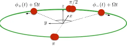
x z π/2

y −

+

φ (t)+ tΩ

π/2 (or )π

φ (t)+ tΩ ⇡/2

⇡

+(t) + ⌦t z (t) + ⌦t x

[image:3.612.185.406.91.174.2]

y

Figure 1. Sketch of the Sagnac interferometer sequence. Theπandπ/2 refers to the two photon pulses.

potentials (TAAPs) [15]. By clock-type interferometer we mean an interferometer, which utilizes two distinct states having different eigenenergies. These potentials have the advantage of being extremely smooth, controllable and flexible. We will examine two types of interferometers, one where atoms propagate freely along a ring-shaped TAAP waveguide and a second where the atoms are fully confined and moved along a circular path. A successful implementation of such an interferometer depends critically on a coherent manipulation of the clock states. Firstly, the clock frequency must not depend on the exact magnitude of the external fields, secondly the transport of the cloud has to be adiabatic, thirdly lifetime of all states involved must be large compared to the duration of the interferometer sequence. It is not clear at this point, whether thermal or Bose-condensed atoms are the best choice for this type of interferometer. Although these issues are important and need to be investigated in detail both theoretically and experimentally, they go beyond the scope of the present paper.

The paper is structured in the following way: Section 2 reviews time averaged potentials and extends them to arbitrary polarization states for interferometry. In section 3 the Sagnac phase is briefly introduced and the different interferometric schemes are presented. TAAP interferometers based on Bragg beams splitters are discussed in section 3.2 while section 3.3 deals with TAAP interferometers based on rf/microwave beam splitters with subsequent state-dependent acceleration (section 3.3.1) or use of moving atom buckets (section 3.3.2). The paper concludes in section 4.

2. The trapping and guiding potentials

2.1. Time averaged adiabatic potentials (TAAPs)

TAAPs can produce extremely controllable and smooth potentials, making them ideal candidates for matter-wave interferometry. They have been proposed in [15] and realised in [11, 16, 17]. In the TAAPs used here, a strong rf-field (Brf) dresses atoms

in a static magnetic quadrupole field (BQ), leading to adiabatic potentials [29]. An

oscillating homogeneous magnetic field (Bm) is then added, which effectively leads to

(4)

potentials. The Hamiltonian for the dressed atoms is then

ˆ

H±=gFµBFˆ.(B(r, t) +Brf(t)) (1)

where ˆFis the total spin of the atoms,µB the Bohr magneton, and gF the Land´e factor.

The ± in ˆH± represents the fact that gF changes sign as (−1)F. We focus on the

|F, mFi=|1,−1i and |2,+1i states of Rubidium 87. For large B-fields these states are

identical with the bare states. We assume that the fields are small enough to neglect the quadratic Zeeman effect.

We combine a static quadrupole field BQ(r) = Bx, By, Bz

= α x, y,−2z

with a homogeneous modulation field which can be tilted by an angle δ from the vertical (z) axis towards the x axis: Bm(t) = Bmsin(ωmt) sin(δ),0,cos(δ)

. The total field is then B(r, t) = BQ(r) + Bm(t). Finally, we add an elliptically polarized rf field

Brf(t) = (B+−B−) cos(ωrft),0,(B++B−) sin(ωrft)

. Note that ωrf itself can be time

dependent, i.e. ωrf(t), with its frequency ωrf ωm typically being in the MHz range.

We define the ellipticity parameter s = (B+ −B−)/(B++B−), where s = 0 denotes

a linear rf in the z-axis, and s = 1 means B− = 0 and thus a pure circular rf in the

x−z plane. In this paper, the polarization will be almost purely linear with a small admixture of circular rf (shh1). The rf field can be understood as the sum of a clockwise (B+) and an anticlockwise (B−) rotating field. We can calculate the coupling rates for

both the F = 2 and the F = 1 hyperfine levels by decomposing the rf field into a basis, which is co-moving with the modulation field. The resulting dressed states will henceforth be referred to as|2,+1i and|1,−1istates respectively. In the rotating wave approximation (RWA), we neglect the component of the rf parallel to the B-field and decompose the orthogonal components into two counter-rotating fields, of which we only use the component that adheres to the conservation of angular momentum‡. The resulting Rabi equation is then:

V±(r, t) = ~ q

[ΩL(r, t)−ωrf(t)]2+ Ω2±(r, t)

' _~Ω±(r, t) +~[ΩL(r, t)−ωrf(t)]

2

2Ω±(r, t)

,

(2)

where ΩL(r, t) =gFµB|B|/~is the Larmor frequency. The Rabi coupling (see Appendix

6) is:

~Ω±(r, t) = ~Ω0

s

1±sBy

|B|

2

−(1−s2₎ B 2 z

|B|2 , (3)

where_~Ω0 = 1₂gFµB(B++B−), the ‘+’ refers to the dressed |2,+1istate and the ‘−’ to

the |1,−1istate. B,By and Bz depend both on r and t.

2.1.1. Experimental Setup: In our experiments, the TAAPs are formed from a quadrupole field, homogeneous time averaging fields, and rf-dressing fields. The

(5)

experiments are performed within a glass vacuum chamber with an estimated pressure in the low 10−11 _{Torr range with a vacuum limited life time of more than two minutes.}

The quadrupole field of up to 400 G/cm is generated using a pair of water cooled coils in anti-Helmholtz configuration. The modulation field oscillates at 5 kHz and can have up to 48 G in amplitude. It is generated by two pairs of rectangular Helmholtz coils in the horizontal and a pair of round coils in the vertical direction. The coils are driven from an eight channel 24 bit sound card, which is amplified using a standard two kilo-watt audio amplifier. In order to control the impedance seen by the amplifier we place capacitors and water cooled 2 Ω resistors in series with the coils. The three interlocking rf-coils each consist of two single loops in Helmholtz configuration. Impedance matching is achieved by placing the pair of coils and the capacitors in parallel. The coils are driven by a 25 W amplifier (Amplifier Research 25A250A), which is controlled by two arbitrary waveform generators (Tektronix AFG3022). Both the rf-coils and modulation coils can produce arbitrarily polarized fields in three dimensions. However, for reasons of experimental simplicity, we keep the frequency of the rf-fields constant. The modulation fields can be changed in amplitude and polarization on a time-scale of 3 ms.

The experimental sequence starts by loading a 3D-MOT with 2×109 _{atoms (}87_Rb₎

from a 2D-MOT. We transfer the atoms to a matched quadrupole time-orbiting potential (TOP). We then compress the trap by first increasing the quadrupole gradient and then lowering the amplitude of the modulation field. At the same time we cool the atoms using radio-frequency (rf) evaporation to a temperature of about 3Tc (with Tc being

the critical temperature). When the modulation field has reached 5 G, we switch on the rf-dressing fields at a frequency of 2.62 MHz and load the atoms into the dressed potential, which we then deform into the ring-shaped trap. Finally, we take resonant absorption images of the atomic clouds using a 4f custom objective and a CCD camera after a short time of flight.

2.2. The ring waveguide (s= 0, δ = 0)

In order to trap the atoms in the vertical direction as well, we add the modulation field

Bm(t). If the frequency of the modulation field (ωm) is fast compared to the trapping

frequency but slow compared to the Larmor frequency, then we can time-average the dressed, modulated quadrupole potential:

V_±eff(r) = ωm 2π

Z 2π/ωm

0

dt V±(r, t) (4)

For a purely linearly polarized rf-field (s = 0) and a purely vertical modulation field (δ= 0) the field is cylindrically symmetric with respect to the z-axis and identical for the

|2,+1iand |1,−1i states. The potential then forms in the x-y plane a ring-shaped trap of radiusR =_~ωrf0/gµBα. For mathematical simplicity we modulate the frequency (ωrf)

and amplitude (B+(t) = B−(t)) of the rf-field such that atr= (R,0,0) it stays resonant

(ΩL(r, t)−ωrf(t) = 0) at a constant Rabi-frequency (Ωrf(r, t) = Ω0c = const.). This

can be achieved using the following time dependencies ωrf(t) = ωrf0

p

(6)

fig_ringFlat.png

y

0 1

OD

x

[image:6.612.123.469.94.249.2]

x OD

Figure 2. Experimental realisation of a ring-shaped TAAP waveguide (s= 0, δ = 0) with Rubidium atoms in the |2,+2i state. The quadrupole gradient isα =50 G/cm with ωrf/2π = 2.62 MHz. The measured Rabi frequency is Ωrf/2π = 215 kHz. The

radius of the ring isR= 570μm.

and Ω0 = Ω0c

p

1 +β2_sin2₍_ω

mt). In the current experiments constant rf-frequency and

amplitude are used. The ring can then be described close to the trap bottom as [15]:

V_ringeff(r, z) = _~Ω0c+

1 2mω

2

r(r−R) 2₊ 1

2mω

2 zz

2 ₍₅₎

with trapping frequencies in the radial and the z axis directions:

ωr=ω0(1 +β2)−1/4

ωz= 2ω0

1−(1 +β2)−1/21/2,

(6)

where β = gFµBBm/~ωrf0 is the normalized modulation index and ω0 =

mFgFµBα (m~Ω0c)

−1/2

.

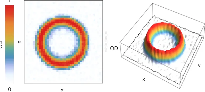
Figure 2 shows an absorption image of 4.8×105 atoms in a TAAP ring of 1.15 mm diameter. Note that the noise in the image is purely due to the imaging system.

An important feature of the TAAP rings is the ability to tune the sensitivity of the interferometer simply by changing either the dressing frequency or the gradient of the static quadrupole field (α), which determine the ring’s radius and therefore the enclosed area. We have demonstrated rings from 400μm to 2.6 mm in diameter filled with up to

6×105 _{atoms at temperatures down to 2}

μK. The life time of atoms in such a trap is of

the order of ten seconds.

Matter waveguides need to be very smooth for the longitudinal motion not to couple to transverse excitations. The TAAP waveguides are formed by rf-dressing of atoms in a quadrupole field generated by large coils rather than from shaping electrical currents using wires. This results in exceedingly smooth waveguides, since the corrugations due to the wires decay exponentially with the distance from the generating coils [30, 31].§

(7)

0.015 0.020 0.025 0.030 0.035 0.040 0.045 0.050 0.0

0.2 0.4 0.6 0.8 1.0 1.2

1/α[Gpcm-1]

Radius

[

mm

]

TAAPρwithα

Inverse Gradient α-1_[cm/G]

R

ad

iu

s

R

[image:7.612.165.420.84.257.2]

[mm]

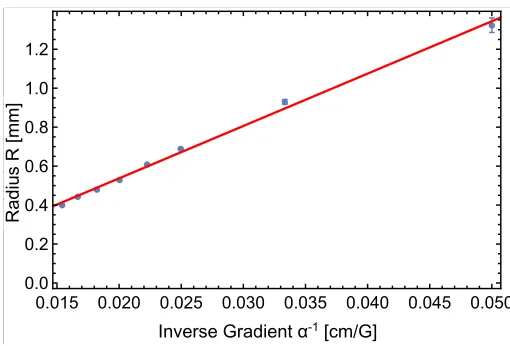
Figure 3. Radius R of the TAAP rings as a function of the inverse magnetic gradient of the quadrupole (1/α) for a constant rf-frequency ofωrf/2π= 2.5 MHz. The

polarization of the dressing RF is circular in the x-y plane, the vertical modulation magnitude is 1.9 G and the Rabi frequency Ωrf/2π = 300 kHz. Note that we do not

modulate the frequency of the rf, and that therefore the radius of the ring is smaller than one might expect (R <~ωrf0/gµBα). The solid red line serves as a guide to the

eye. The error bars correspond to the standard deviation of repeated experiments and is typically∼0.3% of the radius.

This makes TAAP rings extremely smooth and therefore promising candidates for the coherent matter-wave guiding over macroscopic distances and hence for matter-wave interferometry.

2.3. The tilted ring trap (s= 0, δ 6= 0)

The plane of the ring is defined by the direction that the time-averaging field (Bm) is

oscillating in. For δ = 0 the modulation field is vertical and the ring horizontal. For

δ 6= 0 the field tilts towards the x-axis and gravity creates a half-moon shaped trap in the direction of the tilt (see Figure 4). For δhh1, the combination with the gravity field shifts the center of the z-confinement according to z → z0 = z −Rδcosφ/2−g/ω_z2, where φ is the azimuthal angle. By slightly tilting the modulation field Bm from the

purely vertical (0< δhh1) we can tilt the ring thus creating a crescent shaped trap with a potential of

V_geff(r) =V_ringeff (r, z0)− mg

2

2ω2 z

−δ1

2mgRcos(φ). (7) Figure 4(a) shows an experimental realisation of a tilted trap of 1 mm diameter with 3×105 _{Rubidium atoms in the} _|₁_,₋₁_i _{state with} _δ _{= 0}_._{28 rad and Figs. 4(b),(c) are}

ring traps with the same number of atoms and trap conditions, tilted in two opposite directions along the y—z plane.

(8)

a) b) c)

fig_ringTilt3.png

y 0

1

OD x

y y

[image:8.612.75.519.64.234.2]

x x

Figure 4. A tilted ring trap: Experimental realisation of gravity tilted TAAP buckets in |1,−1i state (s = 0) with α = 55 G/cm, ωrf/2π = 2.62 MHz. The radius is R= 500μm and the atom number is about 3×105 atoms. In a)δ = 0.28 rad = 16◦.

In b,c) we tilt the ring in the y—z plane, in opposite directions, by the same amount of 16◦_.

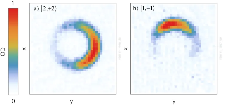
2.4. The state dependent trap (

fig_ringStateF2.png

s6= 0, δ= 0)

y 0

1

x

OD

y

OD

x

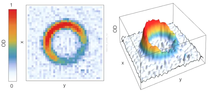
Figure 5. Experimental realisation of a state dependent TAAP bucket (s6= 0,δ= 0) for the|2,+2istate at a quadrupole gradient ofα= 55 G/cm andωrf/2π= 2.62 MHz.

3×105 _{atoms were trapped in the bucket and the radius is}_R_{= 490}

μm.

The Rabi coupling for circular rf polarisation depends on the selection rules for the transition and thus on the state of the atoms. The pure ring trap of Section 2.2 has a strong vertically polarized rf field. Adding to it a small, circularly polarized rf will increase or decrease the coupling strength Ωrf of Eq. 3 depending on which state the

atoms are in (e.g. see Fig. 5 for the particular demonstration of a state dependent TAAP bucket in the |2,+2i state).

For a small positive s, the circular rf component lies in the x-z plane and increases the Rabi frequency of the|2,+1istate in the positive y-direction while at the same time decreases it for the |1,−1i state. This creates a trap located at r = (−R,0,0) for the

[image:8.612.120.471.372.526.2]

(9)

elliptic rf (0< shh1) we obtain to first order:

V_±eff(r) = V_ringeff (r, z)±_~Ω0c

2s

πE(iβ) sinφ , (8)

where E(x) is the complete elliptic function.

2.5. Arbitrary traps (s6= 0, δ6= 0)

y y

0 1

OD x x

fig_ringArb.pdf

[image:9.612.101.486.236.416.2]

a) 2,+2 b) 1,−1

Figure 6. Experimental realisation of arbitrary traps with (s6= 0, δ6= 0) for the two states |2,+2i (5×105 _{atoms) and} _|₁_,₋₁_i ₍₃_×₁₀5 _{atoms) at} _ω

rf/2π = 2.62 MHz.

The fitted radius is 440μm and 450μm respectively. The quadrupole gradient is

α= 55 G/cm. Note that a) and b) are taken with identical experimental conditions and differ only in the state of the atoms. The axis of the circular rf component and the one of the tilted modulation are not orthogonal.

Combining the state dependent potentials (s 6= 0) with a tilt of the modulation field (δ 6= 0), we create two independent traps each at an arbitrary position along the ring (e.g. see Figure 6 for a demonstration with the |1,−1iand |2,+2istates)

The resulting potential is then:

V_±eff(r) =V_ringeff (r, z0)− mg

2

2ω2 z

−V0cos(φ∓φ0) ,

V0 =

s

2

πE(iβ)~Ω0cs

2

+

1 2mgRδ

2

,

tan(φ0) =

4s_~Ω0cE(iβ)

πmgRδ .

(9)

By adjustings andδ, we can adjust the trap positionφ0 to take any value between

(10)

The two traps are anti-symmetric with respect to the x-z plane. Note also that in principle the tilt of the modulation and the weak circular rf component can point in any direction.

The corresponding azimuthal trap frequency

ωφ=

1

R

r

V0

m . (10)

governs the speed at which one can move the two traps around the ring without exciting the trapped atomic cloud.

Figure 6 shows a TAAP with two traps in arbitrary positions. Both images are taken at identical experimental conditions, but with different states: in figure 6a the atoms are in the |2,+2i state and in figure 6b in the |1,−1i state. The axis of the circular rf component and of the tilt are shifted by π/4.

2.6. Landau Zener losses

From equation (6) it is clear that one has an interest in reducing Ω0 and thus Brf in

order to achieve a maximal radial confinement. This however is limited by Majorana spin flips, which occur when the rf-coupling between the energy levels is too weak for the atoms to follow the adiabatic states. According to the Landau-Zener criterion the probability of such transition is given byP = exp(−2πΓ±). Since the time variation of

the potential experienced by the atoms depends mainly on the modulation, rather than the atom’s motion, we obtain according to [15]:

Γ±(r, t) =~

Ω2

±(r, t)

∂t(ΩL(r, t)−ωrf(t))

1 (11)

Assuming a small tiltδhh1 and a low amplitude circular rfs ≤1/p1 +β2 _{then spin flip}

losses are suppressed when:

ωm hh

Ω2_0cR ω aho

, (12)

where aho = (~/mωφ)1/2 is the azimuthal harmonic oscillator length.

3. TAAP Interferometers

Here we discuss the different types of matter-wave interferometers made possible by the TAAP potentials. We start with interferometers using the matter-wave guides of section 2.2 and introduce two different types of beam splitters: one based on Bragg beams (section 3.2) and one based on rf/microwave two photon transitions and state selective manipulation of the atoms (section 3.3). We then show that the latter scheme can also be used in the fully trapped case (section 3.3.2). In order to avoid any contribution other than the Sagnac phase (φ0

S), we ensure that the state-dependent trajectories of

(11)

states in exactly the same internal state. The only difference between the trajectories of the two clouds is then the direction in which the atoms travel.

3.1. Sagnac Interferometry

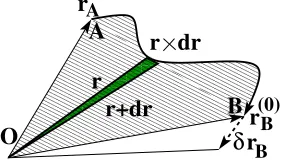
We will shortly review the Sagnac phase as it applies to our guided interferometers. The Sagnac phase occurs in atom trajectories that enclose an area. It is often assumed that the two wave packets overlap perfectly at the second beam-splitter. Insufficient overlap is usually taken into account only as a reduction in contrast. For coherent matter-waves such as those originating from a condensate one can achieve a large contrast even when the overlap is limited [32, 33]. We will show, that in this case there is nevertheless a correction to the Sagnac phases.

00000000000000000 00000000000000000 00000000000000000 00000000000000000 00000000000000000 00000000000000000 00000000000000000 00000000000000000 00000000000000000 00000000000000000 00000000000000000 00000000000000000 00000000000000000 00000000000000000 00000000000000000 00000000000000000 00000000000000000 00000000000000000 00000000000000000 00000000000000000 11111111111111111 11111111111111111 11111111111111111 11111111111111111 11111111111111111 11111111111111111 11111111111111111 11111111111111111 11111111111111111 11111111111111111 11111111111111111 11111111111111111 11111111111111111 11111111111111111 11111111111111111 11111111111111111 11111111111111111 11111111111111111 11111111111111111 11111111111111111 00000000000 00000000000 00000000000 00000000000 00000000000 00000000000 00000000000 00000000000 00000000000 00000000000 00000000000 00000000000 00000000000 00000000000 11111111111 11111111111 11111111111 11111111111 11111111111 11111111111 11111111111 11111111111 11111111111 11111111111 11111111111 11111111111 11111111111 11111111111 000000000000 000000000000 000000000000 000000000000 000000000000 000000000000 000000000000 000000000000 000000000000 000000000000 000000000000 000000000000 000000000000 000000000000 111111111111 111111111111 111111111111 111111111111 111111111111 111111111111 111111111111 111111111111 111111111111 111111111111 111111111111 111111111111 111111111111 111111111111 r r+dr r

r dr A

δr_B

O

A

[image:11.612.224.366.285.365.2]

B r(0)_B

Figure 7. Representation of the area covered by the atoms together with the correction to non adiabaticity.

This can be formulated under the following rather general theorem: We assume non interacting atoms evolving from point A to B with phase accumulation given by Φ±(t).

The starting and end points of the classical trajectory in the absence of rotation are rA and r

(0)

B . The presence of the rotation changes the classical Lagrangian with a

linear correction term δL(t) that induces the change in the classical action governing the phase accumulation. If δrB is the linear correction to the external rotation Ω (see

Fig. 7), then the linear contribution due to this external rotation is given by:

ΦBA=

Z tB

tA

dt δL(t)/_~

= m

~

2Ω.

Z B

A

r×dr+˙r(0)_B .δrB

.

(13)

A proof of this relying only on the classical dynamics of the atom motion can be found in Appendix 7. The first term of equation (13) gives the area enclosed by the atoms while the second gives the correction due to non-adiabaticity. Note that the second term can always be made to vanish by an appropriate choice of origin of the reference frame such that the external rotation motion cancels the final velocity (by adding a term Ω×a, where a is the vector of the new origin). The two clouds accumulate two different corrective phasesδΦB±_A. If we assume that without the external rotation they

[image:11.612.199.455.569.633.2]

(12)

B O

δr_B− −

B+ δr_B+

.

[image:12.612.238.350.89.190.2]

A

Figure 8. The ‘area‘ encircled by the atoms of the two states if the atom trajectories

B−AB+ are not entirely closed. O represents the origin of the coordinate system and is entirely arbitrary.

δΦ = Φ_B+_A−Φ_B−_A

= m

~

2Ω.

Z

A

dS+˙r(0)_B+.δrB+ −˙r(0) B−.δrB−

. (14)

where A is the surface enclosed by the path B−AB+_OB− _and _dS _{is the differential}

surface vector. Please note that the choice of origin O does not change the value of the integral, since the change in area is exactly compensated by the change in

˙r(0)_B+.δrB+ −˙r(0)

B−.δrB−. We retrieve the standard Sagnac formula Φ0

S = 4πΩA

h/m , if at the

end of the interferometer sequence the atoms are at rest and the area is closed, i.e. the atomic clouds overlap fully.

In most Sagnac interferometers the atoms travel along the identical path in opposite directions. In this case the area of the interferometer is the sum of the areas surrounded by each arm and thus twice the area of the single path. Taking the particular case of a ring-shaped interferometer of radius R and radial trapping frequency ωρ and assuming

that the atoms are strongly confined to the ring (ωρΩ) the area is A= 2πR2. Since

r2

B =R2 we find r (0)

B±.δrB± = 0 and due to the tight confinementδrB± = 0.

Therefore, we obtain a much simpler expression

ΦS(T) =

δφ(T)

h/m ΩA =

δφ(T) 4π Φ

0

S , (15)

where δφ(T) = φ+(T) −φ−(T) is the difference in angle between the cloud centers

accumulated during their trajectory along the ring interferometer, with δφ(T) = 4π

signifying therefore the closed area. The Sagnac phase is therefore only affected by the final position of the mass center of the atoms.

For a finite radial confinement we have to take into account that the atoms will experience a centrifugal force during their trajectory, which will be compensated by the radial trapping potential. The area of the interferometer (and thus its sensitivity) will therefore increase slightly. An upper bound for this is

δA

A ≤Max



2

˙

φ0

ωρ

!2

(13)

Taking a transit time of 1 s and a radial trapping frequency of 400 Hz, we find a negligible correction of 10−5_{. Note that this correction affects only the sensitivity and not the}

zero-fringe.

Finally, care needs to be taken to minimise the spread of the wavepackets during their trajectory as well as the influence of the interatomic interactions. For a thermal cloud this can always be done simply by reducing the number of atoms. For a Bose condensed cloud, the phase diffusion rate Rφ can be estimated assuming a Poissonian

atom number fluctuations and a chemical potentialµ taken for a Thomas-Fermi profile [34]:

Rφ=

1

~

√

N ∂µ ∂N

N/2

=

72 125

1/5

a aho

2/5

ωho

N1/10 (17)

whereωho is the geometric average of the trapping frequencies andahothe corresponding

harmonic oscillator length, anda the s-wave scattering length. Surprisingly enough this implies that—as opposed to the thermal case—the phase coherence time of a BEC interferometer increases for increasing atom number even in the case of absence of squeezing, much in contrast to the thermal case.

3.1.1. Guided Sagnac Interferometry: The basic idea of a Sagnac interferometer is that atoms travel in opposite directions around an enclosed area. Due to the resulting common path, the interferometer becomes independent of any static force or acceleration (gravity) but remains sensitive to rotation.

The main challenge for guided Sagnac interferometers is the interaction with the waveguide. In the previous implementations, the smoothes of the waveguide posed serious limitations as it couples the forward motion of the atoms to transverse excitations. In the case of magnetic guiding potentials the shape of the waveguide is defined by the shape of the field generating wires, and therefore, imperfections in the wires translate directly into imperfections of the waveguides. This is the one reason why interferometry in waveguides has only been demonstrated over microscopic distances so far [19, 13, 35]. The TAAPs of this paper, however, are generated from coils that are large and far away. The resulting waveguides are therefore inherently smooth (see section 2.1 and [15]).

(14)

potentials, where even the second order contribution can be cancelled [37, 38]. The ideal dressing and modulation fields of the TAAPs will be investigated separately. However, they interact differently with different polarisations of the rf dressing fields. A σ+

polarized rf field will couple the |1,−1i to the |1,+1i state, but not the |2,+1i to the

|2,−1istate. The opposite is true for aσ− polarized rf. We can therefore use thedegree

of circular polarisation of the rf dressing field in order to manipulate the atoms in a state-dependent fashion.

Combining an elliptically polarized rf-field with a tilt of the ring-shaped waveguide, we can move the two states independently to anywhere on the ring (e.g. Fig. 6) including moving the two clouds around the ring in opposite directions. For such a case the standard Sagnac phase is defined as

Φ0_S = 4πΩA

h/m , (18)

where Ω is the angular velocity of the rotation to be determined, m the mass of the atom and A is the area enclosed by the arms of the interferometer [4, 39]. For the case of the ring-shaped wave guide discussed in this paper, where the two wavepackets travel once around the ring in opposite directions, the area is A = 2πρ, where ρ is the radius of the ring.

The Sagnac formula still holds both for wave-guided interferometers and 3D-trapped atomic clouds. We extend the concept of the area to cases where the paths are not fully closed and consider corrections to the area taking into account the centrifugal forces. As shown previously, the phase accumulation corresponds to the classical action (in units of _~) taken over the trajectory [39].

3.2. A waveguided interferometer with a Bragg beam splitter:

We will first turn our attention to the case of a ring-shaped waveguide interferometer, that uses Bragg beams to split the initial atomic wave packet into two momentum states. Section 2.2 demonstrates the ring-shaped TAAP trapping potentials (s= 0, δ= 0), that will serve as waveguides for the interferometer. In order to place an atom cloud into this waveguide we load a cold thermal cloud or a BEC into the harmonic trap created by tilting the modulation fields (s = 0, δ 6= 0) as discussed in section 2.3. We then switch suddenly to the flat ring (s= 0, δ = 0) and apply a near resonant Bragg pulse, which splits the atomic cloud into two momentum states ±2_~k in the laboratory frame, with k = 2π/λ being the wave vector of the light [40]. The atoms then move along the ring with a constant (angular) velocity ˙φ0±(t) = ±2π/T, where T = 2πR/(2vrec)

is the half round trip time and vrec is the recoil velocity of the Bragg beams. After

(15)

r0±(t) = Rcos[(±2π/T + Ω)t], Rsin[(±2π/T + Ω)t],0

. Since the atoms remain at the trap minimum only the kinetic energy contributes to the phase difference. We obtain a phase shift for a round trip of the two clouds:

Φ±(T) =

mR2

2

Z T

0

dt

~

Ω± 2π

T

2

. (19)

By calculating the phase difference between the two trajectories we recover the standard Sagnac phase of equation (18): ΦS(T) = Φ+(T)−Φ−(T) = Φ0_S. In the more general

case, however, the components have different angular velocities φ±(t) = ˙φ±t, and thus r0±(t) = Rcos[( ˙φ± + Ω)t], Rsin[( ˙φ± + Ω)t],0

. An example is the use of Raman beamsplitters, where the two beams may have different frequencies. This results in the modified Sagnac signal:

ΦS=

2πR2_T

h/m

h

( ˙φ+−φ˙−)Ω + ( ˙φ2+−φ˙ 2

−)/2 i

(20)

Raman pulses in free space offer very precise control over the difference in the velocity of the split atomic clouds. For the case of a TAAP waveguide, however, the alignment of the potential with respect to the optical Raman beams has to be taken into account. In practice this means that the square terms in the Sagnac equation (20) severely limit the precision in the determination of Ω. It is therefore desirable to choose the Bragg scheme, where the two velocities are identical and the non-linear terms vanishes.

3.3. Interferometry based on state dependent manipulation of atoms in a ring

Even though the simplicity of the Bragg scheme is conceptually very appealing, it has the major drawback that the reference for the Sagnac phase is the standing wave of the Bragg beams and thus the retro-reflecting mirror which generates it. Whereas in free-space interferometers this is a very suitable reference, in wave-guided interferometers this poses the problem that this can cause a spurious phase shift when the position of the wave guide moves relative to the one of the retro-reflecting mirror. We therefore have to look for interferometers, where the phase reference is defined by the trapping fields themselves. This is the case for clock type interferometers [27] using as a beam splitter a two photon rf/microwave pulse. The position of the beam splitter is then simply the position of the atoms in the trap.

We start with atoms in the |2,+1i state in the tilted ring described in section 2.3 at the initial angular position φ± = φ0(t = 0) = 0. The atoms are at rest in the

rotating frame, therefore the initial velocity in the inertial frame is ΩR. We then apply a two-photon π/2 pulse, which puts the atoms into an equal superposition of the two dressed hyperfine states |2,+1i and |1,−1i. We then move the atoms half way around the ringk. After half of a round trip we apply a π pulse, which turns the |2,+1i state

(16)

into the |1,−1i state. We then complete the round trip for each of the two states and apply a second π/2 pulse. Due to the π pulse the experimental sequence of the second half can be exactly the time reversal of the first half, thus ensuring perfect symmetry of the whole interferometric sequence. There are two principle options to move the atoms around the ring interferometer: a) the atoms are subjected to an initial state-dependent acceleration and then propagate freely in a TAAP matter-wave guide the static or dynamic accelerator rings described below or b) the atoms are fully confined in three dimensions using themoving buckets of section 3.3.2.

3.3.1. The Accelerator Ring: After preparing the atoms in a superposition of |2,+1i

and|1,−1i, we switch to a state-dependent trap (s6= 0 andδ = 0, as discussed in section 2.4) with the two trap centers at φ0± =±π/2. The |2,+1i and |1,−1i components of

the atom clouds then start to accelerate symmetrically in opposite direction until they reach φ0± = ±π/2, at which point they start to slow down. Due to the symmetry

of the potential the clouds come to a standstill after they have concluded a half turn (φ0± = π). We then apply a π-pulse, which turns |2,+1i into |1,−1i and vice versa.

The atom clouds, now with their identity exchanged, accelerate again and continue to travel in the same direction as before, until they reach φ0± = ∓π/2 and finally

come to a standstill at φ0± = 0. A further π/2 pulse then closes the interferometer,

with the readout being the difference in populations of the |2,+1i and |1,−1i states. Conveniently, these two components separate again and are easily imaged when they reach their maximum separation at φ0± =±π/2. The angle φ±(t) =±φ(t) follows the

nonlinear classical equation (see Appendix B):

mR2φ¨(t) = V0(t) sin(φ0(t)−φ(t)) (21)

and formula (15) still holds.

Since the TAAP waveguides are extremely smooth [15], no transverse modes are excited during the transit and equation (21) yields

T = 2

s

mR2

2V0

Z π

0

dφ

√

sinφ '7.4/ωφ. (22)

With the atoms overlapping and being at rest during the second π/2 pulse, the interferometer is well described by the Sagnac phase ΦS.

The fact that the atoms come to a standstill at φ0± = π causes an unnecessarily

(17)

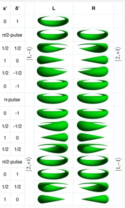
3.3.2. Moving Buckets: In most inertial atom-interferometric measurements the atoms are in free fall for most of the interferometer sequence. Even in the case of the waveguided interferometer described above the atoms are free to travel around the ring. However, as is evident e.g. from equation (14) and described in [27, 28], this is not a strict requirement: atoms in a matter-wave guide or even in a 3-D trap still reproduce the Sagnac phase. Even macroscopic atom clocks flown once around the globe display the Sagnac phase [42]. In the following sections, we describe Sagnac interferometers where the atoms are for most of their trajectories fully 3D-trapped. One important advantage of this is that this prevents the atomic cloud from expanding excessively during its trajectory.

s’ δ’ L R

0 1

π/2-pulse

1/2 1/2

1 0

1/2 -1/2

0 -1

π-pulse

0 -1

1/2 -1/2

1 0

1/2 1/2

π/2-pulse

0 1

1/2 1/2

1 0

2

,

+

1

2

,

+

1

1,

−

1

1,

−

[image:17.612.171.422.257.673.2]

1

Figure 9. A sketch of the isopotential surfaces for the ‘bucket’ traps showing the different stages of transport during the interferometer sequence. s0 and δ0 stand for the degree of tilt and circular polarisation respectively.

(18)

0) = 0 and initial radius R. The atoms are at rest in the rotating frame, therefore the initial velocity in the inertial frame is ΩR. We apply a two-photonπ/2 pulse, which puts the atoms into an equal superposition of the two dressed hyperfine states |2,+1i and

|1,−1i. The two states are then moved in opposite directions for a half of a turn around the ring (φ±(t = T) = ±π). When the atoms are exactly at the opposite side of the

ring, i.e. after a transit timet=T /2 we apply aπ-pulse, which swaps the two hyperfine states. When the full turn is complete (t = T) the atomic clouds are recombined by a second π/2 pulse at φ±(t = T) = ±2π = 0. Note that each of the two wave packets

travel through the exactly same regions of space in the same hyperfine state. In a static inertial frame, the trajectory of the atoms is therefore symmetric with respect to time reversal and with respect to the plane spanned by φ = 0 and the z-axis. The interferometer is therefore not sensitive to any static (inhomogeneous) external field or acceleration (gravity). We realize three dimensional trapping using a combination of the state-dependent and gravitational potentials as described in equation (9). The position of the trap minimum angleφ0(t) expressed in equation (9) is tuned slowly by a variation

of the ellipticity (s parameter) and the rotation (δ parameter) of the modulation field so that the condensates follow the trap center.

Let us first consider an adiabatic transfer of the atoms around the ring. In order for the atoms to remain at the ground state of the trap, the trap frequencies have to be much higher than the typical time variation associated with φ0(t), i.e. ¨φ0(t) << ωφ2.

The position of the atoms is then r±(t) = r0±(t) and the equations (38-40) yield ˙r±(t) = ˙r0±(t) = ~k±(t)/m. Assuming a slow rotation Ω, tight radial confinement,

and that the final velocity of the two atom clouds is zero ( ˙φ0(T) = 0) we get the usual

Sagnac phase shift ΦS(T) = ΦS.

In a real experiment the adiabatic transfer would require an extremely slow acceleration of the trap (Rφ¨0(t) << ω2φ) and a very long transit time (Thh2π/ωφ).

A faster motion would cause the center of mass of the atoms to oscillate with respect to the center of the trap. However, for a harmonic trap this oscillation can be optimally controlled [43]

Let us now look at the case when the trap moves too fast for the adibaticity to be preserved, but slow enough for the atoms to remain within the harmonic limit of the trap. For a trap moving at a constant speed φ0±(t) = ±2π t/T and assuming the atoms

start in the laboratory frame at position φ(0) = 0 and are initially at rest ( ˙φ(0) = 0) we can write down the classical motion of the atoms as

φ±(t) =±2π

t T −

sin(ωφt)

ωφT

˙

φ±(t) =±

2π

T [1−cos(ωφt)]

(23)

If we assume tight radial confinement then equation (15) yields the Sagnac phase

ΦS(T) =

1− sin(ωφT)

ωφT

(19)

Therefore, we recover the standard Sagnac phase (Φ0

S) if the transit timeT is a multiple

of the trap oscillation time (2π/ωφ).

We can also avoid the oscillation by starting with static traps at the position

φ0±(0) =±φa rather than at φ0(0) = 0. A quarter of oscillation period later t=π/2ωφ

the atoms will then be exactly at the trap bottom and move at an angular velocity ˙

φ± =±ωφφa. If at that moment we start to move the trap at the same angular velocity,

then the atoms are transported in the ground state of the trap. Stopping the trap at

φ0±=∓φa and waiting a further quarter of an oscillation period perfectly overlaps the

two atom clouds at zero relative velocity. We therefore measure the standard Sagnac phase. The transit time for this trajectory is then T = _ω2π

φ(1/2−1/π+ 1/φa). This

trajectory guarantees that for most of the transit the atoms are at rest in the moving frame and is much faster than the adiabatic requirement (Thh2π/ωφ).

3.4. Sensitivity

We have demonstrated rings with radius’ ranging from R = 200μm to 1.5 mm. Using

equation (18) with A = 2πR2 we calculate the transfer function or scale factor of a ring-interferometer with a radius R = 1.5 mm to be ΦS/Ω = 4×104rad/(rad/s). The

earth’s rotation of ∼72μrad/s therefore results in a phase shift of ΦS '3 rad.

Numerical simulations for a condensate in our experimental conditions indicate that the Sagnac phase can be preserved for atom numbers as large as a few thousand [44], resulting in a shot noise limited phase resolution of tens of milli radians. Given our repetition rate of a few tens of seconds, we expect a sensitivity of 10−5_rad/s/Hz1/2_.

According to [27] also thermal atoms can be used. In that case, using 106 _{thermal atoms}

at a repetition rate of 1 Hz and pushing the ring diameter to one centimeter a sensitivity of 10−9_rad/s/Hz1/2 _{will be reached.}

4. Conclusions

We demonstrated and analysed ring-shaped potentials for ultra-cold atoms and propose different schemes for its use in Sagnac interferometry. We demonstrated that using an elliptical polarization of the rf-field in combination with gravity we can arbitrarily and dynamically manipulate two different spin states at the same time.

(20)

(21)

5. Bibliography

[1] Carnal O and Mlynek J 1991Physical Review Letters 662689–2692

[2] Keith D W, Ekstrom C R, Turchette Q A and Pritchard D E 1991 Physical Review Letters 66

2693–2696

[3] Kasevich M and Chu S 1991 Physical Review Letters 67181–184

[4] Barrett B, Geiger R, Dutta I, Meunier M, Canuel B, Gauguet A, Bouyer P and Landragin A 2014

Comptes Rendus Physique15875 – 883 [5] Will C M 2006 Living Reviews in Relativity 9

[6] Igel H, Cochard A, Wassermann J, Flaws A, Schreiber U, Velikoseltsev A and Pham Dinh N 2007

Geophysical Journal International 168182–196

[7] Tino G and Kasevich M 2014 Interferometry with atoms (interferometria atomic)Proceedings of the International School of Physics Enrico Fermi (Varenna, Italy, 2014) (Societ`a Intaliana di fisica, Bologna, Italy)

[8] Berg P, Abend S, Tackmann G, Schubert C, Giese E, Schleich W, Narducci F, Ertmer W and Rasel E M 2015Phys. Rev. Lett.114063002

[9] Bongs K, Burger S, Dettmer S, Hellweg D, Arlt J, Ertmer W and Sengstock K 2001 Comptes Rendus De L Academie Des Sciences Serie IV 2671–680

[10] Henderson K, Ryu C, MacCormick C and Boshier M G 2009NEW JOURNAL OF PHYSICS 11

043030

[11] Heathcote W H, Nugent E, Sheard B T and Foot C J 2008New Journal of Physics 10043012 [12] Hansel W, Hommelhoff P, Hansch T W and Reichel J 2001Nature 413498–501

[13] Schumm T, Hofferberth S, Andersson L M, Wildermuth S, Groth S, Bar-Joseph I, Schmiedmayer J and Kruger P 2005Nature Physics 157–62

[14] Dumke R, Muther T, Volk M, Ertmer W and Birkl G 2002Physical Review Letters 89 220402 [15] Lesanovsky I and von Klitzing W 2007Physical Review Letters 99083001

[16] Sherlock B E, Gildemeister M, Owen E, Nugent E and Foot C J 2011Physical Review A83043408 [17] Gildemeister M, Nugent E, Sherlock B E, Kubasik M, Sheard B T and Foot C J 2010 Physical

Review A81 031402

[18] Gildemeister M, Sherlock B E and Foot C J 2012Physical Review A85053401

[19] Wang Y J, Anderson D Z, Bright V M, Cornell E A, Diot Q, Kishimoto T, Prentiss M, Saravanan R A, Segal S R and Wu S J 2005Physical Review Letters 94090405

[20] Berrada T, van Frank S, Backer R, Schumm T, Schaff J F and Schmiedmayer J 2013 Nature Communications 4

[21] Schumm T, Manz S, B¨ucker R, Smith D A and Schmiedmayer J 2011Interferometry with Bose– Einstein Condensates on Atom Chips (Wiley-VCH Verlag GmbH & Co. KGaA) chap 7, pp 211–264 ISBN 9783527633357 URLhttp://dx.doi.org/10.1002/9783527633357.ch7

[22] Henkel C, Kruger P, Folman R and Schmiedmayer J 2003Applied Physics B 76173–182

[23] Trebbia J B, Garrido Alzar C L, Cornelussen R, Westbrook C I and Bouchoule I 2007 Physical Review Letters 98263201

[24] Sinclair C D J, Curtis E A, Garcia I L, Retter J A, Hall B V, Eriksson S, Sauer B E and Hinds E A 2005Phys. Rev. A72031603

[25] Bohi P, Riedel M F, Hoffrogge J, Reichel J, Hansch T W and Treutlein P 2009Nature Physics 5

592–597

[26] Guarrera V, Szmuk R, Reichel J and Rosenbusch P 2015New Journal of Physics17083022 URL

http://stacks.iop.org/1367-2630/17/i=8/a=083022

[27] Stevenson R, Hush M R, Bishop T, Lesanovsky I and Fernholz T 2015 Phys. Rev. Lett.115(16) 163001 URLhttp://link.aps.org/doi/10.1103/PhysRevLett.115.163001

[28] Fernholz T, Gerritsma R, Kr¨uger P and Spreeuw R J C 2007Phys. Rev. A75063406 [29] Zobay O and Garraway B M 2001Physical Review Letters 861195–1198

(22)

URLhttp://dx.doi.org/10.1038/nature06149

[31] Della Pietra L, Aigner S, vom Hagen C, Groth S, Bar-Joseph I, Lezec H J and Schmiedmayer J 2007Phys. Rev. A75063604 URLhttp://dx.doi.org/10.1103/PhysRevA.75.063604

[32] Andrews M R, Townsend C G, Miesner H J, Durfee D S, Kurn D M and Ketterle W 1997Science

275637–641

[33] Jo G B, Shin Y, Will S, Pasquini T A, Saba M, Ketterle W, Pritchard D E, Vengalattore M and Prentiss M 2007Physical Review Letters 98030407

[34] Javanainen J and Wilkens M 1997Phys. Rev. Lett.784675–4678 URLhttp://dx.doi.org/10. 1103/PhysRevLett.78.4675

[35] Ockeloen C F, Schmied R, Riedel M F and Treutlein P 2013 Physical Review Letters 111(14) 143001 URLhttp://link.aps.org/doi/10.1103/PhysRevLett.111.143001

[36] Harber D M, Lewandowski H J, McGuirk J M and Cornell E A 2002 Physical Review A 66(5) 053616 URLhttp://link.aps.org/doi/10.1103/PhysRevA.66.053616

[37] Kazakov G A and Schumm T 2015Phys. Rev. A91023404

[38] Sárkány L, Weiss P, Hattermann H and Fortágh J 2014 Physical Review A 90 053416 URL

http://dx.doi.org/10.1103/PhysRevA.90.053416

[39] Antoine C and Bord´e C 2003Physics Letters A 306277

[40] Giltner D M, Mcgowan R W and Lee S A 1995Physical Review Letters 752638–2641

[41] Buggle C, Leonard J, von Klitzing W and Walraven J T M 2004Physical Review Letters93173202 [42] Hafele J C and Keating R E 1972Science 177168–170 (Preprint http://www.sciencemag.org/ content/177/4044/168.full.pdf) URL http://www.sciencemag.org/content/177/4044/ 168.abstract

[43] Gu´ery-Odelin D and Muga J G 2014 Phys. Rev. A 90(6) 063425 URL http://link.aps.org/ doi/10.1103/PhysRevA.90.063425

[44] Trombettoni A 2015 Private communication

(23)

6. Appendix A: Determination of the potential

6.1. Coupling field calculation

To determine the effective potential felt by the atoms, we use the rotating wave approximation (RWA) i.e. we assume that only the polarized component of this field rotating perpendicularly to the quadrupole field effectively interacts with the atoms. This perpendicular component is given by:

B⊥_rf(r, t) =Brf(t)−

Brf(t).B(r, t)

|B(r, t)|2 B(r, t) . (25)

This component rotates at the frequency ωrf with an elliptical polarization:

B⊥_rf(r, t) = B1cos(ωrft) +B2sin(ωrft) (26)

where

B1 = (B++B−)

−BzBx |B|2 ,−

BzBy

|B|2 ,1−

B_z2

|B|2

, (27)

B2 = (B+−B−)

1− B

2 x

|B|2,−

ByBx

|B|2 ,−

BzBx

|B|2

. (28)

It can be rewritten in the equivalent form:

B⊥_rf(r, t) = B01cos(ωrft+χ) +B02sin(ωrft+χ) (29)

with a phase shift χ chosen such as to fulfill the orthogonality of the amplitudes

B01.B02 = 0. This last condition together with the comparison between the two last

expressions Eq.(26) and Eq.(29) allow to find the following identities:

B01

B02

!

= cosχ −sinχ sinχ cosχ

!

. B1

B2

!

(30)

and

tan(2χ) = 2B1.B2

B2 2−B21

. (31)

Rewriting the amplitude of these field as |B01| = B+0 +B−0 and |B02| = B+0 −B−0 , we

can identify the new parameters as the effective Rabi coupling _~Ω±(r, t) =gµBB±0 and

recover the equation (3).

(24)

7. Appendix B: Non adiabatic interferometry

In this appendix we discuss how to calculate the phase evolution of the atoms during their trajectory inside the ring. We show that, if the atoms are at rest in the beginning and end of the interferometric sequence, then the resulting phase depends only on the area enclosed and is essentially independent of the dynamic evolution of the atoms within the interferometer. We generalize the Sagnac formula (13) for the case that the trajectories do not fully enclose an area.

7.1. The Sagnac phase in a travelling harmonic trap

We assume that the interactions between the atoms are negligible so that the atomic clouds in the two states|2,+1iand|1,−1ievolve according to the Schr¨odinger equation for the atoms in the inertial frame:

i_~∂tψ±(r, t) =−~

2

2m∇

2

rψ±(r, t) +V±(r−r0±(t), t)ψ±(r, t), (32)

where the atoms are trapped in the moving harmonic potential V±(r − r0±(t), t)

centered at the position r0±(t) whose dynamics can be chosen arbitrarily.

For the particular ring trap configuration, we use the dynamics r0±(t) =

{Rcos [±Ωt+φ0(t)],±Rsin [±Ωt+φ0(t)],0} so that the potential equation (9) is now

rewritten in the inertial frame by taking into account of the external rotation angle Ωt

that is added or subtracted to the angle of the trap minimum φ0(t) in the laboratory

frame. In the trap center frame, the harmonic potential has the local form:

V±(r, t) =

m

2r.ω

2

±(t).r

T ₍₃₃₎

and depends on the trap position φ0(t) through the tensor of the trap frequencies:

ω2_±(t) =O(Ωt±φ0(t)).



 

ω2

r 0 0

0 ω2 φ 0

0 0 ω2 z





.O

T

(Ωt±φ0(t)) (34)

where we used the rotation matrix:

O(φ) =



 

cos(φ) −sin(φ) 0 sin(φ) cos(φ) 0

0 0 1





 (35)

This description can also be used for a ring shaped waveguide, with ωφ = 0 and the

trajectory of the trap center φ0(t) being chosen such that it follows the free evolution

of atom cloud. We use the following transformations:

ψ±(r, t) =ei[k±(t).(r−r±(t))+Φ±(t)]ψ0±(r−r±(t), t) (36)

to rewrite the Schr¨odinger equation in the moving frame of the position of the atom wave packet center r±(t) as

(25)

This is achieved if this position r±(t) obeys the dynamic equations:

˙r±(t) =~k±(t)/m (38)

~k˙±(t) = −

∂V(r±(t)−r0±(t), t)

∂r±(t)

(39)

Φ±(t) =

Z t

0

dt0

~

L(r±(t0),˙r±(t0), t)

L±(r±(t),˙r±(t), t) =

1 2m˙r

2

±(t)−V(r±(t)−r0±(t), t). (40)

This result is strictly only valid for a harmonic potential and is thus a good approximation for atoms located close to the trap center |r±(t) − r0±(t)|hhR (see

Appendix 7.3). As a consequence of the Kohn transformation that extends the translational invariance transformation concept to the case of the harmonic trap [45], the center of mass position of the condensate center evolves according to the classical Lagrangian L±(r±(t),˙r±(t), t) [39]. The transformation applied here to cartesian

coordinates can be generalized to any time-dependent harmonic potential for any coordinates choice like the cylindrical coordinates developed in Appendix 7.3 provided the resulting potential can be assumed quadratic in these coordinates.

7.2. Proof of the non adiabatic area theorem

Let us suppose the rotation of angular velocity Ω of the laboratory frame. Then the laboratory coordinatesrL(t) are related to the inertial coordinates through the relation

rT(t) = O(Ωt)rT_L(t) where we define the rotation matrix O(Ωt) about the angular velocity at angle|Ωt|. In this frame, the classical motion equation of an atom under an external potential V(r(t), t) becomes:

m(¨rL(t) + 2Ω×r˙L(t) +Ω×(Ω×rL(t)) = −

∂V(rL(t), t)

∂rL(t)

(41)

Making the perturbative development rL(t) =r(0)(t) +r(1)(t) +. . . up to the first order

in the angular velocity and applying it to Eq.(41), we determine the correction to the action perturbatively. Suppose a classical motion between time tA and tB, we calculate

successively:

Z tB

tA

dtS(rL(t),r˙L(t), t)

=

Z tB

tA

dthm

2( ˙rL(t) +Ω×rL(t))

2₋

V(rL(t), t)

i

=

Z tB

tA

dtS(0)(r(0)(t),r˙(0)(t), t) + 2mΩ.

Z r(0)(tB)

r(0)_(t

A)

r(0)×dr(0)+m˙r(0)(t).r(1)(t)|tB

tA

(26)

7.3. Anharmonic treatment

We generalize the results of section 7.1 to the case of an anharmonic equation. In the case of strong radial confinement, the Schroedinger equation in the inertial frame is simplified into:

i_~∂tψ±(φ, t) = [− ~2∂φ2

2mR2 −V0(t) cos(φ∓φ0(t)−Ωt)]ψ±(φ, t).

(43)

Similarly to the harmonic treatment, the azimuthal part of the trap potential (9) written in the inertial frame is centered about ±φ0(t) + Ωt. Thus according to the hyperfine

components, it accounts for the external rotation angle Ωt that is added or substracted to the trap minimum angle φ0(t). For the symmetric case where the atom components

evolve in opposite directions, the following transformation

ψ±(φ, t) = ei[l±(t).(φ−φ±(t)−Ωt)+Φ±(t)]ψ0±(φ−φ±(t)−Ωt)

(44)

rewrites the Schroedinger equation in the moving frame of the atoms as:

i_~∂tψ0±(φ, t) =

− ~

2_∂2 φ

2mR2 +V0(t)[(1−cos(φ)) cos(φ0(t)∓φ±(t))

−(sinφ−φ) sin(φ0(t)∓φ±(t))]

ψ0±(φ, t) (45)

provided the following conditions are fulfilled:

˙

φ±(t) =~l±(t)/mR2−Ω, (46)

mR2φ¨±(t) = −V0(t) sin(φ±(t)∓φ0(t)), (47)

Φ±(t) =

Z t

0

dt0

~

L±(φ±(t),φ˙±(t), t),

L±(φ±(t),φ˙±(t), t) = ~

2_{( ˙}_φ

±(t) + Ω)2

2mR2 +V0(t) cos(φ0(t)∓φ±(t)).

(48)

With the boundary conditions φ±(0) = ˙φ±(0) = 0, we recover the formulae (15)

whatever the dynamics involved. Let us note that l±(t) should strictly speaking be

an integer since the wave function should be periodic in φ. However as long as the radius is much larger than the spatial extension of the wave function (Raho), it can

be extended to the real value domain. Under the condition of a localized wave function, the equation (45) is simplified into an harmonic oscillator:

i_~∂tψ0±(φ, t) =

− ~

2_∂2 φ

2mR2 +V0(t) cos[φ0(t)∓φ±(t)]

φ2

2

ψ0±(φ, t) (49)

where the effective trap frequency is time dependent:

(27)

In order to avoid further phase accumulation, strictly speaking, one has to ensure the adiabaticity of the evolution of the wave function. The main limitation is the transition to the excited state in the trap which is negligible when the transit timeT is much longer than the time variation of the trap frequency i.e.Tω˙eff

φ±(t)/ωφeff±(t)hh1. All these conditions

fulfilled, we recover using (48) the formula (15) whatever the dynamics involved. In practice, these conditions are only fulfilled in the bucket case where using Eq.(23) we find ωφT 1. Nevertheless, this additional phase accumulation is not important as it

cancels out in the phase difference if we restrict the calculation in the linear contribution in Ω.

8. Appendix C: Contrast

The atom profile after recombination at the second π/2 pulse at time t is altered when the wave packets coming from the two arms are not synchronized. The contrast resulting from these imperfections can be determined quantitatively from the atom density obtained for the two states after interferometry:

P±(r, T) =

1

4|ψ+(r, t)±ψ−(r, t)|

2

. (50)

Because of the high confinement in along the radial direction, we neglect the effect of the internal rotation inside the trap during the interferometry process. Using Eq.(36) together with the ground state wave function:

ψ0±(r) =

mω_ho

π_~

3/4

exp[−m

2_~r.ω±(t).r

T

] (51)

and ωho = (ωrωzωφ)1/3, we obtain after integration the probability of the two hyperfine

states after interferometry:

P±(T) = Z

d3rP±(r, T)

= 1 2

1± V(T) cos

ΦS(T)−

k+(T) +k−(T)

2 .δr(T) (52) where we define the visibility:

V(T) = exp

"

−m

2_δ_r₍_T₎_.ω

±(t).δr

T₍_T_{) +}_δ_k₍_T₎_.ω−1

± (t).δk

T₍_T₎

4_~m

#

(53)

depending on the mass center position δr(t) = r+(T) −r−(T) and the momentum

differenceδk(t) =k+(T)−k−(T). The contrast of the interferometer will be reduced, if

the two wave packets originating from the two arms of the interferometer have a finite velocity relative to each other or if they do not overlap perfectly at the final beam splitter. In the case of a tight confinement within the ring, the probability simplifies into:

P±(T) =

1 2 ±

V(T) 2 cos

"

ΦS(T)−

mR2

~

˙

φ+(T) + ˙φ−(T)

2 (δφ(T)−4π)

#

(54)