FINE-SCALE DISTRIBUTION OF CARBOHYDRATES
ON INTERTIDAL SEDIMENTS IN RELATION TO
DIATOM BIOMASS AND SEDIMENT PROPERTIES
Irene Sarah Taylor
A Thesis Submitted for the Degree of PhD
at the
University of St Andrews
1998
Full metadata for this item is available in
St Andrews Research Repository
at:
http://research-repository.st-andrews.ac.uk/
Please use this identifier to cite or link to this item:
http://hdl.handle.net/10023/14233
FINE-SCALE DISTRIBUTION OF CARBOHYDRATES ON INTERTIDAL SEDIMENTS IN RELATION TO DIATOM BIOMASS AND SEDIMENT
PROPERTIES
Irene Sarah Taylor
A thesis submitted in partial fiilfilments of the requirements for the degree of Doctor of Philosophy, at the University of St Andrews.
School of Environmental and Evolutionaiy Biology, University of St Andrews,
ProQuest Number: 10166226
All rights reserved INFORMATION TO ALL USERS
The quality of this reproduction is dependent upon the quality of the copy submitted. In the unlikely event that the author did not send a com plete manuscript and there are missing pages, these will be noted. Also, if material had to be removed,
a note will indicate the deletion.
uest
ProQuest 10166226
Published by ProQuest LLO (2017). Copyright of the Dissertation is held by the Author. All rights reserved.
This work is protected against unauthorized copying under Title 17, United States C ode Microform Edition © ProQuest LLO.
ProQuest LLO.
789 East Eisenhower Parkway P.Q. Box 1346
ST ANDREWS UNIVERSITY
Declarations
I, Irene Sarah Taylor, hereby certify that this thesis which is approximately 45,000 words in length, has been written by me, that it is the record of work carried out by me and that it has not been submitted in any previous application for a higher degree.
I was admitted as a research student in September 1994 and as a candidate for the degree of Doctor of Pliilosophy in October 1995; the higher study for which this is a record was carried out in the University of St Andrews between 1994 and
1997.
(oj %!
9
A chwwledgements
I am very grateful to my supervisor David Paterson for his advice on all aspects o f this study, for his good example andfor always finding the time.
I would also like to thank all the members o f the SERG team for their friendship and encouragement; Irvine Davidson for his advice and patient
teaching o f low-temperature scanning electron microscopy and photography. Claire Honeywill and Julie Kelly fo r explaining the quirks o f the HPLC system and providing me with data for comparative studies. Trevor Tolhurst for digging me out o f the mudflats and Kevin Blackfor providing me with several useful references. I would also like to acknowledge Mireille Consalvey and Steve Shayler for their cheerful team spirit. In addition, Karen Wiltshire and Alison Miles for their help and advice at the beginning o f this study and James Blackburn for laboratory and software advice. Furthermore, I thank Jan Lorenzen for his assistance during my visit to Aarhus.
A special thanks to my family fo r all their help and support and to Andrew for the welcome distractions.
CONTENTS
ABSTRACT...viii
LIST OF FIGURES...ix
LIST OF TABLES...xiv
LIST OF ABBREVIATIONS...xvi
CHAPTER 1________________________________________________________ 1 1. GENERAL INTRODUCTION... 2
LI INTERTIDAL DEPOSITIONAL ENVIRONMENTS... 2
1.2 EXTRACELLULAR POLYMERIC SUBSTANCES (EPS)... 5
1.3 EPS SYNTHESIS...7
1.4 THE FUNCTIONS OF EPS... 8
J. 4.1 Habitat stabilisation...8
1.4.2 Sessile adhesion.^...9
1.4.3 EPS as a carbon source and binding agent...9
1.5 CONCLUSION... 10
CHAPTER 2_______________________________________________________ U 2. MATERIALS AND METHODS... 12
2.1 SITE SELECTION... 12
2.1.1 The Eden Estuary ...12
2.1.2 The Humber Estuary...17
2.2 THE QUANTIFICATION OF CARBOHYDRATES...18
2.2.1 Introduction ... 18
2.2.2 Testing and modifying the assay protocol...21
2.2.3 A protocol for the measurement o f colloidal carbohydrates... 23
2.2.4 A protocol for the measurement of bulk carbohydrates... 25
2.2.5 The calculation of carbohydrate concentration...25
2.2.6 Repeated extractions...26
2.3 COLLECTION OF SEDIMENT SAMPLES...28
2.4 FINE-SCALE SECTIONING OF SEDIMENTS... 30
2.4.2 A protocol for fine scale sectioning of sediment... 30
2.4.3 The use offilter paper for the transfer of sediment sections...31
2.5 A PROTOCOL FOR THE EXAMINATION OF DIATOM ASSEMBLAGES USING THE LIGHT MICROSCOPE...36
2.5.1 Isolation of in situ diatom cells...36
2.5.2 Slide Preparation...36
2.6 SCANNING ELECTRON MICROSCOPY... 37
1.1 PARTICLE SIZE ANALYSIS...37
2.8 THE MEASUREMENT OF CARBOHYDRATES IN ASSOCIATION WITH DEPLOYMENT OF GUST’S MICROCOSM ...38
2.8.1 Introduction...38
2.8.2 In situ microcosm deployment...39
2.8.3 The measurement of carbohydrates in sea water... 41
2.8.4 Results...43
2.8.5 Discussion...43
2.8.6 Second microcosm field deployment...47
CHAPTER 3 MICROSPATIAL VARIATION IN CARBOHYDRATE FRACTIONS WITH SEDIMENT DEPTH________________________49 3. INTRODUCTION... 50
3.1 MATERIALS AND METHODS...54
3.1.1 Sites...54
3.2 RESULTS...55
3.2.1 Microscale carbohydrate depth profiles... 55
3.2.2 Spatial variation...59
3.3 DISCUSSION...69
3.3.1 Carbohydrate fractionation... 69
3.3.2 Microscale depth profiles... 69
3.3.3 Spatial variation... 73
CHAPTER 4 TEMPORAL VARIATION IN SEDIMENT CARBOHYDRATE I
I
CONCENTRATIONS OVER TIDAL EMERSION PERIODS________ 76
4. INTRODUCTION... 77
4.1 MATERIALS AND METHODS... 80
4.1.1 Low-temperature scanning electron microscopy (LTSEM)... 82
4.1.2 Protocol for carbohydrate assays ...82
4.2 RESULTS...82
4.2.1 Variation o f carbohydrate concentrations over the emersion period.... 82
4.2.2 Measurements of physico-chemical factors over the emersion period...89
4.2.3 Extracellular enzyme activity... 91
4.2.4 Sediment stability.... 91
4.2.5 Measurements of daily variation... 95
4.3 DISCUSSION... 95
4.3.1 Conclusions... 101
CHAPTER 5 COLLOIDAL CARBOHYDRATE CONCENTRATION AND DIATOM BIOMASS IN RELATION TO LIGHT INTENSITY 102 5. INTRODUCTION. ... 103
5.1 METHODS...105
5.1.1 Construction of microelectrode systems...105
5.1.2 Laboratory experiment...106
5.1.3 Field study....Ill 5.2 RESULTS...113
5.2.1 Variation in measured parameters over the experimental period.... 123
5.3 DISCUSSION - LABORATORY STUDY... 128
5.3.1 The relationship between light intensity and benthic productivity... 128
5.3.2 The correlation between carbohydrates and chlorophyll a...132
5.3.3 Sediment water content and wet bulk density... 133
5.4 BAIE DE MARENNES-OLÉRON...133
5.4.1 Results...133
5.4.2 Discussion...142
CHAPTER 6 BIOCHEMICAL CHARACTERISATION 0 ¥ IN SITU
CARBOHYDRATE FRACTIONS______________________________ 147
6. INTRODUCTION... ...148
6.1 METHODS... 152
6.1.1 Carbohydrate fractionation... 153
6.1.2 Carbohydrate quantification... 153
6.1.3 Carbohydrate purification for GC-MS analysis... 153
6.1.4Monosaccharide analysis : Methanolysis and GC-MS. ...154
6.2 RESULTS... 155
6.2.1 Monosaccharide GC-MS analysis....155
6.3 DISCUSSION... 159
6.4 CONCLUSION...163
CHAPTER 7 GENERAL DISCUSSION_______________________________UA 7. GENERAL DISCUSSION... 165
7.1 THE SCALE OF ECOLOGICAL MEASUREMENT... 169
7.2 MICROSCALE DISTRIBUTION OF SEDIMENT CARBOHYDRATES 171 7.3 MICROSCALE STUDIES OF SEDIMENT FABRIC. ... 175
7.3.1 The effect of moisture content on the dynamics of carbohydrate fractions 177 7.4 TEMPORAL VARIABILITY OF CARBOHYDRATE CONCENTRATIONS DURING EMERSION ON INTERTIDAL MUD FLATS...177
7.5 BIOCHEMICAL CHARACTERISATION OF/AOTU SEDIMENT CARBOHYDRATE FRACTIONS... 179
7.5.1 Environmental factors which may affect colloidal carbohydrate turnover 181 7.6 A CONCEPTUAL MODEL OF CARBOHYDRATE DYNAMICS ON SURFACE SEDIMENTS... 182
7.6.1 An established biofilm... 182
7.6.2 Following deposition... 185
7.6.3 Following erosion... 185
7.7 FUTURE STUDIES... 186
7.8 CONCLUSIONS... 187
APPENDIX \ . Microelectrode construction... 190
REFERENCES... 192
ABSTRACT
Extracellular polymeric substances (EPS) are produced by epipelic diatoms as a function of their locomotive mechanism and also protect cells from desiccation and heavy metal toxicity. EPS are carbohydrate-rich and form an important carbon source for heterotrophic microorganisms. In addition, the polymeric structure of EPS results in sediment inter-grain binding, thereby increasing the resistance of sediments to erosion forces. Despite the importance of generic carbohydrates (measured as an index of EPS), there is little information on their spatial distribution or factors influencing their abundance. In this study, a fine-scale sectioning technique was developed and provided the first depth profiles of sediment carbohydrates at a scale relevant to microphytobenthos. The
operational separation of sediment carbohydrates into bulk and colloidal fractions was examined and fractions were shown to vary in spatial and temporal
characteristics. Colloidal carbohydrates were concentrated in the surface 200 pm layer of intertidal mud flats and therefore influenced sediment interface processes such as diffusion and sediment erosion. Colloidal carbohydrates were positively correlated to sediment chlorophyll a concentrations and also varied with tidal height and with sediment topography. During the emersion period, colloidal carbohydrate concentrations increase significantly, however, bulk carbohydrate concentrations remain unchanged. Biochemical analysis of the carbohydrate fractions showed marked, but not statistically proven, differences in the
LIST OF FIGURES CHAPTER 1
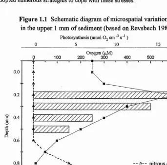
Figure 1.1 Schematic diagram of typical microspatial variation in the upper 1 mm...2
CHAPTER 2
Figure 2.1 The location of Eden and Humber Estuaries...13 Figure 2.2 An aerial photograph of the Eden Estuaiy...15 Figure 2.3 A map of sediment distribution in the Eden Estuaiy... 16 Figure 2.4 Detail of the Skeffling sampling site on the Humber Estuary showing
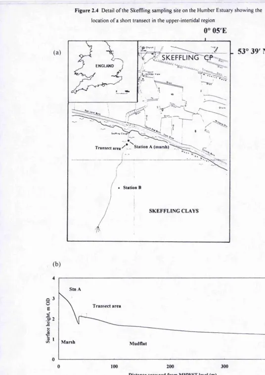
the location of a short transect in the upper-intertidal region... 19 Figure 2.5 A map of sediment distribution for the Humber Estuary...20 Figure 2.6 The absorbance peak of glucose in the Dubois assay... 22 Figure 2.7 (a) Comparison of 3 glucose standards (b) comparison of different
volumes using the same proportion of glucose to phenol ... 24 Figure 2.8 Repeated extractions of sediment colloidal carbohydrates...27 Figure 2.9 Repeated extraction of colloidal carbohydrate (Underwood et al.
1995)...29 Figure 2.10 Wet mass concentration values derived using brush or filter
paper...32 Figure 2.11 Depth profiles of wet mass concentration using both methods 34 Figure 2.12 A comparison of methods to remove carbohydrates from filter
paper...35 Figure 2.13 An illustration of the microcosm device...40 Figure 2.14 Artificial separation of carbohydrate fractions...42 Figure 2.15 (a) colloidal and (b) particulate carbohydrate concentrations in the
water column... 44 Figure 2.16 Suspended particulate matter over an erosion event... 45 Figure 2.17 Comparison of absorbances from standard curves before and after
freeze drying... 46
CHAPTER 3
Figure 3.1 Regression analysis of colloidal carbohydrates (log 10+1 transformed) with depth on 3 intertidal mud flats (linear regression with 95 %
confidence limits)...56 Figure 3.2 Regression analysis of bulk carbohydrates (log 10 transformed) with
depth in the upper 10 mm (log 10) on 2 intertidal mud flats on the Humber Estuary (linear regression with 95 % confidence limits.)... 58 Figure 3.3 Microscale depth profiles of dry mass concentration within the upper 2
mm at Hawkins Point, Skeffling and Guardbridge mud flats (error bars are 2 X SEM, n = 12, 4 and 6 respectively)...60 Figure 3.4 A microscale depth profile of dry mass concentration in the upper 20
mm at Hawkins Point (error bars are 2 x SEM, n = 12)... 61 Figure 3.5 Low-temperature scanning electron micrographs of surface sediments from Hawkins Point...62 Figure 3.6 A spectra of particle size diameters of surface sediments along a 3
point transect at Skeffling...64 Figure 3.7 Percentage moisture content of surface sediments along a 3 point
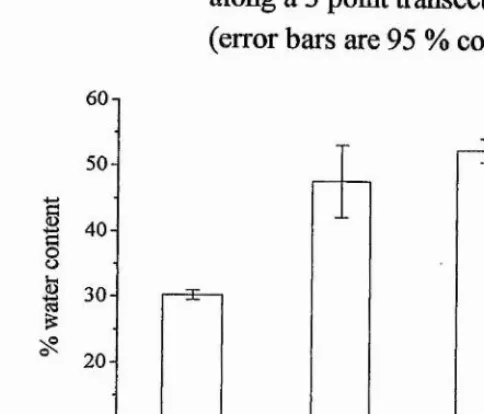
transect at Skeffling (error bars are 95 % confidence limits, n = 3)... 64 Figure 3.8 (a) Dry mass concentration of surface sediments along a downshore
transect (error bars are 2 x SEM, n = 3). (b) Colloidal carbohydrate concentrations along the transect (error bars are 2 x SEM, n = 5)... 65 Figure 3.9 Colloidal and bulk carbohydrate concentrations in the upper 5 mm of a runnel and ridge at Skeffling (error bars are 2 x SEM, n = 6)...67 Figure 3.10 The wet and dry mass concentrations of sediment in the upper 5 mm
of a ridge and runnel at the Skeffling site (error bars are 2 x SEM,
n = 2)...68 Figure 3.11 Schematic diagram showing the distribution of carbohydrate
fractions, dry mass concentration and porosity in the upper 10 mm, based on microscale depth profiles at Hawldns Point...71 CHAPTER 4
Figure 4.2 Location of sampling sites on the Eden Estuary... 81 Figure 4.3(a) Colloidal carbohydrate concentrations over the emersion period
at site A and (b) site B on the Humber Estuary...83 Figure 4.4 Temporal and spatial study of colloidal carbohydrates on the Humber
Estuaiy... 85
Figure 4.5 Concentrations of bulk carbohydrates over the emersion period on the Humber Estuary... 86 Figure 4.6 Temporal variation in colloidal carbohydrate concentrations at (a)
site 1 and (b) site 2 on the Eden Estuary...87 Figure 4.7 Microscale depth profiles of colloidal carbohydrate distribution over
the tidal emersion period...88 Figure 4.8 Temporal variation in dry mass concentration at the Eden Estuary...90 Figure 4.9 Percentage water content in surface sediments over the emersion
period at sites 1 and 2 at the Eden Estuary... 92 Figure 4.10 Temporal variation in extracellular enzyme activity on surface
sediments of the Humber Estuary...93 Figure 4.11 Sediment stability during the emersion period at the Humber
Estuary... 94 Figure 4.12 Low-temperature scanning electron micrographs of surface
sediments from the Eden Estuary...96 Figure 4.13 Schematic diagram showing processes which influence the
concentrations of sediment colloidal carbohydrates... 99 CHAPTER 5
Figure 5.1 Methods for measuring primaiy productivity...104 Figure 5.2 Oxygen microelectrode with guard cathode (left), fast response and
sturdy, slow response oxygen microelectrodes (right)... 107 Figure 5.3 Photographs of (a) mid-intertidal and (b) upper-intertidal sites at
Baie de Marennes-Oléron (courtesy of Claire Honeywill)... 112 Figure 5.4 Chlorophyll nr, colloidal carbohydrates and oxygen productivity at 4
light intensities on Day 1... 114 Figure 5.5 Chlorophyll a, colloidal carbohydrates and oxygen productivity at 4
light intensities on Day 4...115
Figure 5.6 Chlorophyll a, colloidal carbohydrates and oxygen productivity at 4 light intensities on Day 6...116 Figure 5.7 Chlorophyll a, colloidal carbohydrates and oxygen productivity at 4
light intensities on Day 8... 118 Figure 5.8 (a) Colloidal carbohydrate and (b) chlorophyll a concentrations in
sediments at 4 light intensities pooled over the time series...119 Figure 5.9 Colloidal carbohydrate concentrations at each light intensity
normalised to chlorophyll a concentrations... 120 Figure 5.10 Depth profile of oxygen concentrations and primary production in
the upper 5 mm of a sediment core... 121 Figure 5.11 The distribution of oxygen in the upper 4 mm of sediment cores at
varying light intensities... 122 Figure 5.12 Net average oxygen production rates at variable light intensities... 124 Figure 5.13 Net average oxygen production rates normalised to chlorophyll a at
varying light intensities... 125 Figure 5.14 Variation in sediment water content between different light
intensities...126 Figure 5.15 (a) Temporal variation in oxygen productivity and (b) wet sediment
density with time...127 Figure 5.16 Conceptual model showing the effect of initial algal biomass on
subsequent growth in (a) dark conditions (b) low light and (c) optimum light intensities... 131 Figure 5.17 Depth profile of colloidal carbohydrate concentrations on
mid-intertidal sediments at Baie de Marennes-Oléron (10/4/97)... 134 Figure 5.18 Depth profile of colloidal carbohydrate concentrations on
upper-intertidal sediments at Baie de Marennes-Oléron...135 Figure 5.19 Decrease in algal biomass with sediment depth at the mid-intertidal
site...137 Figure 5.20 Depth profiles of chlorophyll a over the emersion period on
upper-intertidal sediments at Baie de Maremies-Oléron...138 Figure 5.21 Low-temperature scanning electron micrographs of sediments from
CHAPTER 6
Figure 6.1 The range of carbohydrate forms present on intertidal sediments.... 149 Figure 6.2 Total Ion Chromatograms (TIC) of the GC-MS carbohydrate analysis, a) sugar standards (b) colloidal carbohydrate sample (c) bulk carbohydrate sample (Gal: galactose, Glu: glucose, Man: mannose, Xyl: xylose, Rha: rhamnose, si: 5c>»//c>-inositol) ...156 Figure 6.3 The variation in monosaccharide composition (%) of bulk and
colloidal samples... 157 Figure 6.4 Total ion chromatographs (TIC) illustrating the effect of TFA
purification on sample integrity during GC-MS analysis...158 Figure 6.5 Hypothesised structure of epipelic diatom EPS...161 CHAPTER 7
Figure 7.1 Aerial photograph showing the spectral reflectance of
microphytobenthic chlorophyll at Skeffling mud flats (Courtesy of Kevin Morris)...166 Figure 7.2 Low-temperature scanning electron micrographs showing (a) increase
in sediment density with sediment depth and (b) the large size range of epipelic diatom cells...167 Figure 7.3 Conceptual diagram showing how migration may influence the
surface concentration of colloidal carbohydrates...183
LIST OF TABLES
CHAPTER 1
Table 1.1 A comparison of spectrophotometric carbohydrate assays...6 CHAPTER 2
Table 2.1 A comparison of the organic content of smffcial intertidal
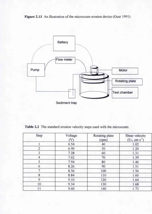
sediments... 15 Table 2.2 The standard erosion velocity steps used with the microcosm... 40 CHAPTERS
Table 3.1 Carbohydrate concentrations measured in natural sediments...51 Table 3.2 Mean concentrations of colloidal carbohydrate... 57 Table 3.3 Mean concentrations of bulk carbohydrate...57 Table 3.4 Variation in carbohydrate concentration with tidal level on two
intertidal mud flats...66 CHAPTER 4
Table 4.1 Variations in light and temperature over the emersion period 89 Table 4.2 Measurements of primary production and light intensity on the Humber
Estuary...89 CHAPTER 5
Table 5.1 Oxygen microelectrode dimensions and performance...106 Table 5.2 The solvent gradient used in HPLC pigment analysis...I l l Table 5.3 A comparison of modelled net and measured gross photosynthetic
rate... 123 CHAPTER 6
Table 6.1 The concentration of individual monosaccharides identified in each carbohydrate fiaction... 159 Table 6.2 Comparison of monosaccharide abundances in water column and
sediment samples... 162 CHAPTER 7
Table 7 2 Comparisons of the gradient of colloidal carbohydrate decline with ... 174 depth...
ARRREVIATTONS AND SYMBOLS
C dry mass concentration (kg m'^, also known as dry density, pa) CSM cohesive strength meter
D sediment apparent sediment diffusion coefficient (cm s )
D water water diffusion coefficient (cm ^ s )
EPS extracellular polymeric substances GC-MS gas chromatography-mass spectrometry HPLC high-performance liquid chromatography
J flux (according to Pick’s 1st Law of Difiüsion, nmol O2 c m 's ‘)
test statistic for Jonckerre’s test of ordered alternatives LISP Littoral Investigation of Sediment Properties
LOIS Land Ocean Inter-action Study LN2 liquid nitrogen
LTSEM low-temperature scanning electron microscopy Ms mass of solids (kg)
NAPR net average production rate (nmol cm s ) NMR nuclear magnetic resonance
PAR photo synthetically active radiation (400-700 nm) rpm revolutions per minute
SE standard error (also known as standard error of the mean, SEM) SD standard deviation
SPM suspended particulate matter (g 1 ^) TIC total ion chromatograms
TFA tri-fluoracetic acid
UDOM ultrafiltered dissolved organic matter
U *crit critical shear velocity (m s'^)
V volume (m’^)
X p h depth of photosynthetic zone
0 porosity
Ter critical erosion stress (N m*^)
Unrestricted copyright
In submitting this thesis to the University of St Andrews I understand that I am giving permission for it to be made available for use in accordance with the regulations of the University Library for the time being in force, subject to any copyright vested in the work not being affected thereby. I also understand that the title and abstract will be published and that a copy of the work may be made and supplied to any bona fide library or research worker.
/o/e/^9
Chapter 1____________________________________________________________ General Introduction
Chapter 1 General Introduction
1. General Introduction
1.1 Intertidal depositional environments
[image:22.613.116.459.389.728.2]Intertidal mud flats are complex, highly productive environments which serve as important feeding grounds for migrating birds and juvenile fish. In addition, they are highly dynamic systems which may undergo erosion or deposition with each tidal cycle. Regular exposure to the air results in rapid temperature changes and desiccation of intertidal regions. The tidal variation in exposure leads to large scale gradients or zonation across the surface of intertidal flats. Microsensors studies have also shown significant microscale variation in light and sediment oxygen, sulphide and nitrous oxide concentrations in the upper millimetres of intertidal and subtidal sediments (Fig. 1.1) (Jorgensen et al 1983, Kühl and Jorgensen 1994). These microscale gradients may vary in response to local conditions and biological activity. Therefore, surface sediments contain extreme and rapidly changing microclimates and organisms growing there have adopted numerous strategies to cope with these stresses.
Figure 1.1 Schematic diagr am of microspatial variation in the upper 1 mm of sediment (based on Revsbech 1989).
Photosynthesis (nniol O, cm s'* )
5 10 15
0.2
0.4
0.6
0.8
1.0
Oxygen (jiM)
500
_ _ A - - nitrous oxide ■
—a— oxygen
V //\ photosynthesis “ I '--- 1--- 1--- 1--- '--- 1--- '--- 1--- r
10 20 30 40 50
Chapter 1_______________________________________________ General Introduction
Diatoms (Badllariophyceae) are well suited to growth in dynamic
conditions and are often the main primary producers in depositional environments. In addition, diatoms colonise saltmarsh sediments, plants and any submerged surfaces. Diatoms contribute to 20-25 % of global primary production (Hoek et a l 1995). The annual production of fixed carbon by diatoms in temperate oceans is 200-400 g C and the amount of carbon fixed by a maize crop is 1000-2500 g C m'^ y (Hoek et al 1995). An understanding of the dynamics and ecology of estuarine mud flat systems is a fundamental requirement to predict the
consequences of human activities and the influence of global environmental change in coastal waters.
Diatoms growing on sands have been termed “epipsammic” and those which thrive in mud have been termed “epipelic” diatoms (Round 1971). Most benthic diatoms (both epipelic and epipsammic) range in size fiom 10 pm to 300
pm and are commonly pennate (symmetrically lanceolate) (Admiraal 1984), whereas, planktonic diatoms are dominated by centric forms (radially symmetrical, Admiraal 1984).
Diatoms have adapted to withstand a wide range of temperatures and light intensities. For example, laboratoiy studies have shown Na\ncula salinarum and
N. pygmaea to divide equally rapidly when grown at 15, 100 or 700 pE m'^ s'^ (Admiraal et a l 1984). However, on intertidal sediments, winter and summer species can often be identified (Colijn and Dijkema 1981) suggesting ecological factors other than light may influence natural communities. Estuarine diatoms can grow at salinities between 4 and 60 %o (Admiraal 1984). This tolerance is
Chapter 1____________________________________________________________ General Introduction
forces) resulting in a more stable environment for benthic diatoms. However, epipelic diatoms must cope with the lower porosities of muds and the consequent limitation of oxygen and light, which may penetrate only the upper 0.4 - 0.8 mm (Jorgensen et al, 1983, Kühl and Jorgensen 1994).
During photosynthesis, conditions of high pH, low CO2 availability and
saturated oxygen concentrations commonly occur on intertidal diatom biofilms (Jorgensen et al. 1983, Admiraal 1984). Diatoms cope with these stresses by exhibiting some characteristics of C4 or CAM metabolism (i.e. (3 carboxylase
activity and low values) which may contribute to their success on intertidal flats (Morris 1980, Schwinghammer e/a/. 1983, Admiraal 1984). Another defence against changing environmental conditions and grazing is the ability to exist as resting cells. These resting stages are more suited to long periods of low- temperatures and short photoperiods than parental vegetative cells (McQuoid and Hobson 1995). However, the production of resting cells is almost entirely limited to centric diatoms and the lack of resting cells among pennate diatoms cannot be attributed to more favourable conditions but rather the possession of alternative protection against environmental changes, such as migration (see below).
Intertidal sediments hold plentiful nutrient supplies for autotrophic growth and diatoms, in turn, support a wide range of meiofauna and macrofauna
including the amphipod Corophium volutator, the polychaete worm Nereis diversicolor, nematodes, copepods, harpacticoids and ostracoids (Montagna et al.
1995, Smith et al. 1996). One strategy to cope with this grazing pressure and other environmental stresses is the development of migration patterns. The diatom migratory rhythm is influenced by both lunar and solar cycles and diatoms surface shortly after the sediments are exposed and return (1-3 mm) down into the sediment before tidal inundation (Perldns 1960, Hay et a l 1993, Paterson et al. in review). This allows diatom cells to receive sufficient light for photosynthesis without the risk of being resuspended by the incoming tide (Palmer and Round
1967). The locomotive force for motility in diatoms involves the secretion of polymeric fibrils (extracellular polymeric substances, EPS), across the
Chapter 1____________________________________________________________ General Introduction
maintaining a distal connection to the plasmalemma. Actin filaments in the cytoplasm are thought to act on the fibril attachment site to move the fibrils along the raphe fissure. Since the fibrils are also attached to external objects, the cell is displaced (Drum and Hopkins 1966, Edgar and Pickett-Heaps 1984). The migration pattern and speed of motility has been found to vary among species (Round 1979b, Hay et a l 1993). For example, Gyrosignia limosum (fonnally G.
spemerii) can move across sediments at a speed of 17 mm h'^ and was notably faster thsinNitzschia or Naxncida sp. (Hay et ah 1993). Furtheimore, Happey- Wood and Jones (1988) found greater average speeds mPleurosigina angulatum
during the time corresponding to low tide (32.4 mm h'^) and slower speeds during tidal immersion(9 mm h'^), although this has not been verified in subsequent studies.
1.2 Extracellular polymeric substances (EPS) and colloidal carbohydrates
The copious production of EPS by motile diatoms makes them the most likely source of colloidal carbohydrates in the intertidal zone. Hoagland et al.
(1993) defines EPS as any macromolecule secreted external to the plasmalemma. In addition, non-motile diatoms commonly produce EPS in the form of stalks, pads and cell coatings (Hoagland et al. 1993).
EPS has been examined using many analytical techniques and
histochemical stains have shown EPS from 30 taxa to consist of carbohydrates which are carboxylated or sulphated to varying degrees (Decho 1990, Hoagland
et al 1993 and references therein). These carbohydrates may be structurally altered with NaCl (Alan et al. 1972) resulting in structural variation within an estuary. The monosaccharide composition of the carbohydrates have been identified using separation techniques including paper, liquid, gas-liquid and gas chromatography - mass spectrometry (GC-MS) ( Handa and Mizuno 1973, Cowie and Hedges 1984, Sigleo 1996, McCarthy et al 1996). In addition, nuclear magnetic resonance (NMR) has provided information on colloidal carbohydrates isolated from many different water bodies and has shown the molecules to have very similar linkage and branching patterns (Mcloiight et al 1997). The
Chapter 1 General Introduction
Spectrophotometric assays have been employed for the rapid
quantification of carbohydrates. The phenol-sulphuric acid assay (Dubois et al.
1956) has advantages over other rapid techniques (Table 1.1) since pentoses are detected as well as hexoses. Furthermore, the reaction agents are not affected by other organic materials or inorganic ions present in the marine environment (Handa 1966). Therefore, the phenol-sulphuric acid assay remains the most commonly used assay (Underwood and Smith 1998b, Sutherland 1996).
Diatom carbohydrates have been artificially separated into fractions depending on their solubility (Alan et al. 1972, Haug and Myklestad 1976, Underwood et al. 1995). Firstly, those carbohydrates which are soluble in water and an insoluble fraction. Colloidal carbohydrates are those extracted in aqueous solution and remaining in solution following centrifugation and they are measured as an index of EPS. Approximately 20-25 % of colloidal carbohydrates are polymeric and the other carbohydrates are monomers or short chains. The majority of biochemical studies on algal polysaccharides have involved
[image:26.613.89.489.425.664.2]carbohydrate extractions fi*om planktonic mono-cultures (Hoagland et al. 1993, Alan e/a/. 1972).
Table 1.1 Comparison o f spectrophotometric carbohydrate assays.
Assay Author/s Comments
Phenol-sulphuric
Aitlirone-sulphuric
N-etliylcarbazole
L-tryptophan
MBTH*
Dubois eï'fi/. 1956
Spiro 1966
Lewis & Rakestraw 1955
Grasshoff 1978
Johnson & Siebuith 1977
simple, stable and sensitive (Handa 1966)
antlirone imstable in sulphuric acid, expensive
affected by non-carbohydrate materials (McLauglin et al.
1960)
reaction not chemically understood
many addition steps highly toxic
*3 methyl-2-benzothiazolinone hydrazone
Chapter 1______________________________________________________ General Introduction
and galactose with glucose, mannose, xylose and arabinose present to a lesser extent (Hoagland et ah 1993 and references therein, Allan et al. 1972). In this study the composition of in situ sediment carbohydrates associated with benthic diatoms were investigated for the first time. EPS represents 11-39 % of cellular carbon during stationary phase and 2-8 % during exponential growth (Claus
1988). Laboratory findings suggest that diatom cells produce more EPS in the stationary growth phase than during exponential growth (Myklestad and Haug 1972). In addition, EPS is often produced in greater concentrations in conditions of high nitrate to phosphate ratios, where nutrients are available but perhaps not in the ratios necessary for growth (Myklestad and Haug 1972).
1.3 EPS synthesis
The internal mechanism of synthesis and release begins with cytoplasmic vesicles adjacent to the Golgi apparatus (Edgar 1980). Variation in vesicle morphology suggests progressive stages in synthesis and preparation for secretion. In the case of fibril synthesis, vesicles containing fibrilai' material migrate to the plasmalemma where fusion occurs and the vesicle contents are released into the raphe fissure (Herth 1979, Sicko-Goad et ah 1989).
Radiolabelled uptake studies suggest that the percentage of photoassimilated carbon used to produce EPS is low (0.18-0.48 %, Underwood and Smith 1998).
Since high concentrations of EPS are produced by motile cells,
Chapter 1_________________________________________ ________ __________ General Introduction
1.4 The Functions of EPS
As well as motility, EPS allows habitat stabilisation, sessile adhesion, colony formation and protection against desiccation and toxic substances.
1.4.1 Habitat stabilisation
Diatoms have long been associated with a reduction in the resuspension of sediments (Delgado et al. 1991). In early work, the stabilisation effect was only found to be significant for diatoms which secreted mucilage (Holland et al. 1974) and in a more recent study, a positive correlation was found between colloidal carbohydrates (an index of EPS) and the critical shear velocity (U* crit) (Grant and Gust 1987, Sutherland 1996). These authors speculate on the possible use of this relationship as a means to predict erosion thresholds. Furthermore, in some cases, biological activity can have a greater effect on sediment stability than physical parameters such as bulk density, which are typically used to predict stability (Sutherland 1996).
The stabilisation effect of EPS occurs as diatoms migrate through the sediment causing EPS to accumulate, forming a matrix in the upper millimetres which increases inter-grain binding. There is no information on the fate of EPS or colloidal carbohydrates when sediments are under erosion stress, whether they uncouple from the sediment fabric and enter the water column before sediment erosion or remain associated with sediment particles and settle out after erosion. The drying of sediments over the emersion period increases the stability of surface sediments. In addition, drying may stimulate the production of more EPS
(Peterson 1987) which would further stabilise the sediment, a positive feedback mechanism. Furthermore, EPS smoothes the surface sediment, reducing shear stress and turbulence, thus contributing to stability (Delgado et al. 1991). EPS release creates a more stable environment for the assemblages, preventing
Chapter 1________________________________________________________ General Introduction
1.4.2 Sessile adhesion
Diatoms also use EPS to adhere to submerged surfaces where they can maintain a stable position and where nutrient levels may be greater than in the water column (Brock and Madigan 1991). Diatoms are the most common biofouling microalgae found on submerged surfaces (Characldis and Cooksey
1983). The attachment strength and concentration of EPS was found to vary with the surface tension of the submerged material (Becker 1996). In addition, EPS concentration is reduced by cathodically polarising the surface and tins procedure is used to protect marine structures fiom biofouling and corrosion (Bhosle et al.
1994). EPS secretion in the form of apical pads allows colony formation in many planktonic forms e.g. Asterionella formosa. The formation of a colony structure may reduce the sinking rate and affect the longevity of a diatom bloom.
1.4.3 EPS as a carbon source and binding agent
EPS and colloidal carbohydrates are an important carbon source for the microbial community (Freeman and Lock 1995) and they may encourage the establishment of complex bacterial communities (Stehr et al. 1995).
Heterotrophic bacteria degrade EPS, colloidal carbohydrates and other organic matter using extracellular enzymes, notably a amylase, a and P-glucosidase (Decho 1994). The production of these enzymes varies diurnally and seasonally, mirroring changes in diatom biomass and ambient temperatures (Meyer-Reil 1983, Karner and Rassoulzedegan 1995, Ruddy et a l 1996). Furthermore, ion
exchange across the EPS matrix results in the incorporation of inorganic nutrients (Freeman and Lock 1995). The anionic nature of EPS and colloidal
carbohydrates makes them highly adsorptive to cationic metals such as Zn, Co, Cu, Fe, A1 and Ni (Dugan 1987, Decho 1994, Stehr et al. 1995). These metals are toxic to cells. However, the high metal binding affinity of EPS and colloidal carbohydrates prevents metal uptake into the cell. Similarly, chlorinated
Chapter 1____________________________________________________________ General Introduction
advantage to these cells in biofilms where competition for light and nutrients occur (Hudon and Bourget 1981).
1.5 Conclusion
It is apparent that EPS and colloidal carbohydrates are important in many biogeological and physical processes. Yet, very little is known of the spatial distribution of EPS or carbohydrate fractions within surface sediments. This may be partly due to the difficulties associated with non-destructive analysis and sampling of soft sediments. While the processes of primary production, respiration and denitrification can be measured at a microscale of 100 pm (Revsbech 1989a), there is no device available to quantify similar microscale variations in EPS production and the distribution of caibohydrates.
Carbohydrates may influence many of the biogeological processes which vary significantly over short distances, therefore, a knowledge of the microspatial distribution of carbohydrates would improve our general understanding of sediment ecology. In addition, there is no information regarding microscale properties of the physical environment in which epipelic diatoms occur, such as sediment density or water content. This study aims to address these shortfalls by firstly, characterising the sediment environment at the scale relevant to the microorganisms using low-temperature SEM and high-resolution sectioning techniques and secondly, by conducting parallel measurements of carbohydrate concentrations. This study seeks to provide biochemical information on in sitv
carbohydrate fractions commonly measured and to assess this information in the context of heterotrophic degradation processes involving extracellular enzymes. Such information is necessary for determining the lability of EPS and
carbohydrates in sediments and the likelihood of long-term effects. In addition, the possible influence of some environmental conditions on the distribution of carbohydrates on intertidal mud flats will be addressed through the use of laboratory experiments and the applications of non-destructive sampling methods.
General methods
Chanter 2 : _______________________ -— --- —
Chapter 2: General methods
2. Materials and Methods
2.1 Site selection
The three main field sites were selected, two on the Humber Estuary and one site on the Eden Estuary (Figure 2.1). Background data including sediment origin, nutrient concentrations, diatom migration behaviour were available for the Eden Estuary (Perkins
1960, Ahmad 1990, Mathieson and Aktins 1995). In addition, data on sediment transport, bathymetry, nutrient loading and infaunal species composition were readily available for the Humber Estuary.
2.1.1 The Eden Estuarv
The Eden Estuary is the main research site used by the Sediment Ecology Research Group (SERG) of St Andrews University since it is a local estuary with reasonable vehicular access. At the time of this research, the Eden Estuary was
designated as a primary investigation site for an EU environment programme, PROMAT, allowing multi-disciplinary studies to be carried out. The Eden Estuary, (56° 22’ N 02° 51’ E) is a small estuary situated between St Andrews and the Firth of Tay. The total area of the estuary is 8 km^ and the majority of this area is exposed at low water with the
exception of the narrow channel of the River Eden. The maximum height of water above the central channel does not exceed 5 m and the hydrodynamics are dominated by tidal currents rather than wave action. This is due to the presence of a sand bar across the mouth of the estuary and acts to reduce the force of storm waves (Wilson 1910). Fine sediments are brought into the estuary with the flood tide and are deposited on the tidal flats during the still period of high water.
The human population affecting the estuary is 11 , 0 0 0 and the estuary is important
for local paper manufacturing, fishing and wading birds and waterfowl. The numbers of migrating birds exceeds 16000 and includes a significant percentage of the UK Shelduck, Redshank and Oyster Catcher populations. There are two sites of special scientific interest (SSSI) and an important dune system nature reserve adjacent to the Estuary. Part of the River Eden has been identified as a nitrate vulnerable zone under the EC directive 91/676/EEC (Scottish Office 1994) and the estuary is likely to be affected by eutrophication (Mathieson and Aktins 1995). A review of Scottish Estuaries showed the Eden Estuary to have the highest concentrations of total oxidised nitrogen between
Figure 2 1 The location o f the Eden and Humber Estuaries in the UK
The Eden Estuary
L c u c h a n
Mid-Mertidal futioa
I km
The Humber Estuary
Uvei
Patrington
Hawkins Point
Skeffling Gays
Grimsby
10 km
[image:33.619.25.548.13.748.2]Chapter 2:__________________________________________________ General methods
1990-1994 ( 8 mg TON T*, Mathieson and Aktins 1995). 75 % of the estuary catchment
land is agricultural and the high nutrient concentrations may be due to the increasing use of inorganic fertilisers in cereal crop farming.
2.1.1.1 Sediment biological communities
Sediment fauna in the Eden Estuary includes marine polychaete worms (Nereis diversicolor and Arenicola marina), the amphipod Corophium voluiaior and the
gastropod Hydrohia ulvae. In addition, there are mussel beds on areas of fine sediments. Mussels are known to produce mucopolysaccharides (MPS) to facilitate the processing of suspended particles (Beninger and St Jean 1997). The MPS associated with mussels and other invertebrates may contribute to carbohydrate concentrations on intertidal flats however, this has not been investigated. The primary producers present in the Estuary include the seagrass (Zostera spp.j, macroalgae (Fucus sp., Enterornorpha spp. and Ulva
spp.y) and microalgae. Enterornorpha forms extensive blooms in the spring which remain until late summer on most intertidal flats. The degradation o îEnterornorpha blooms may be a seasonal source of carbohydrates on intertidal flats. The fact the algal growth continues over the summer months suggests that the Enterornorpha growth may be due to high nutrient concentrations in the estuary (Mathieson and Aktins 1995, European Communities 1991). Zostera can be seen to fringe saltmarshes along the margins of north and south shores and Fucus spiralis exists only on boulders and extends up to Guardbridge paper mill. The dominant microphytobenthos are diatoms
(Bacillariophyceae) which often form biofilms in the surface layers although cyanobacteria (mainly Oscillatoria spp.) are often present.
2.1.1 . 2 Sediment characteristics
The mud flats extend 100-300 metres to the Eden River channel and are
bordered at the high shore with a sea-wall of boulders (Figure 2.2). The sediments of the estuaiy are heterogeneous and grain size increases towards the estuary mouth where 90 % of the sediments are quartz material. The upper estuary contains muds and silty sands (Figure 2.3). The organic content of the Eden sediments are within the range of other estuaries (Table 2.1) and increase with decreasing grain size (Ahmad 1990). The organic content of sediments at Baie de Marennes-Oléron was more than double the sediments of the Eden Estuary and this may be because the average particle size at Baie de
Q 2
!
!
(U g W -c
I
I
I
- e < ^ rn gg g
.s p |
Chapter 2: General methods
Oléron sediments was 25 jim compared with 75 pm on the Eden mud flats. There is a wide range of particle sizes at the sampling site (from < 2 pm to > 2 0 0 pm diameter) and
the sediment exhibits cohesive behaviour. The sediment bed is generally flat with occasional minor drainage channels (< 0.5 m wide) in the middle and upper Estuary. Table 2.1 A comparison o f organic content o f surficial intertidal sediments (± standard
deviation).
Estuarv % Organic content Study Sampling month
Eden, Scotland 3.17 ±0.46 Honeywill and
Kelly pers. comm. April 1997 Tay, Scotland 2.68 ± 0.02 Honeywill and
Kelly pers. comm. April 1997 Montrose Basin,
Scotland 0.1-10 Ahmad 1990 1990
Humber, England 2.1 ±0.04 Black pers. comm. April 1995 Marennes- Oléron
Bay, France 6.7 ±0.14 Kelly pers. comm.Honeywill and April 1997 2.1.2 The Humber Estuarv
The Humber Estuary is much larger than the Eden, the width at the mouth is 8 km
and according to the National Rivers Authority (1993), it is the major UK freshwater input into the North Sea. The range of a spring tide is 7 m with current speeds of 2-3 m s'^ (Gameson 1982). Therefore, the estuary is well mixed with little vertical stratification (Black 1996). However, there is cross-stratification between the North and South shores due to an asymmetric tidal inundation pattern. Saline flood waters enter predominately on the north shore whereas freshwater discharges mainly along the south shore. The River Humber has high concentrations of suspended sediments and supplies 200,000 tonnes of sediment to the estuary but this passes out into the North Sea as a plume layer (Pethick 1988). The sediments which form the tidal flats are believed to originate from erosion of cliffs on the Holdemess Coast (north of the Humber Estuary) and be
transported into the estuary during the flood tide (Black pers. comm ).
The sites on the North coast of the Humber Estuary were Hawkins Point (53® 38’ N 0® 3’ W) and Skefrling Clays, (53® 38.5’ N 0° 4.25’ E). Skeffling Clays consists of
Chanter 2: ________________________________________________________________ Gênerai methods
shore and were connected by an anchored wooden walkway (Figure 2.4 a, b). At site A there was an additional 9 metre transect.
2.1.2.1 Biological components
Hawkins Point and Skeffling Clays are similar in their biology, a salt marsh containing Spartim towmendii, Halimiom and Ptwcimllia fringes the mud flats on the North shore (Brown 1996). The sediments are highly active and contain a variety of infaunal species including; Nereis diversicolor, Hydrobia spp., Macoma balthica, Pygospio elegans and to a lesser extent Corophium voluiaior (Morris 1994). Macoma balthica was the most common animal on the Skeffling mud flats (Davey and Partridge
1998). Smaller Mflcowa were found at the high and low-shore with larger sized animals at mid-shore. There was greater bioturbation at site B than at site A due to the increased size of the Macoma (Davey and Partridge 1998). Bioturbation was evident as feeding activity, the presence of faecal pellets and through the construction of burrows. The main primary producers on the mudflats are microphytobenthic communities containing
Euglena spp. and several genera of diatoms {Bacillariophyceae). There were also patches of the macroalgae, Enterornorpha spp.
2.1.2.2 Sediment characteristics
Boulder clay deposits lie underneath the tidal flats at a depth of 0.6 - 4 m and influence channel formation on the over-lying sediments. There was a gradient of particle sizes on the mud flats with finer particles at the topshore and coarser grains towards the central channel (Figure 2.5). At Skeffling site A, the sediment bed was characterised by planar areas and other areas where small ridges and runnels, reaching 1 0 cm in height,
were found. There was a non-consolidated surface layer (approx. 2 cm) which was comprised of fine sediments. Underlying this layer were coarse, black, sandy muds and in some areas, patches o î Macoma balthica shells. At site B, the sediment composition appeared to be homogenous within the upper 10 cm. At both sites there were many low lying areas where surface pools remained thi oughout the emersion period.
2.2 The quantification of carbohydrates 2.2.1 Introduction
Carbohydrates occurring in sediments were quantified using a spectrophotometric assay (Dubois ei al. 1956). This was chosen above other methods (see Chapter 1) since it is least affected by other compounds and it is rapid and simple (Handa and Mizuno
Figure 2.4 Detail o f the Skeffling sampling site on the Humber Estuary showing the location o f a short transect in the upper-intertidal region
0° 05'E
(a)
Æ .S K E FFLIN G
E N G U V N D
Transect a r e * S t a t i o n A (marsh)
S t a t i o n B
SKEFFLING CLAYS
(b )
Stn A
Transect area
Stn B
Marsh Mudflat
200 300 400
0 100
HUMBER ESTUARY
10 kilom étras
7 sta tu te m iles
7 nautical m iles (latitude m inutes)
KEY TO C O L O U R S &
Easington
303
S h o u l
9 2 0 1
9155
[image:40.618.27.547.18.683.2]Spurn Head
Figure 2.5 Distribution of seabed sediments for the Humber estuarv with particular reference to the intertidal area within Spurn Bight (from British Geological Survey maps SPURN Sheet 53°N-00° and HUMBER-TRENT Sheet 53°N-02W°, I; 100 000).
Chapter 2:________ General methods
1973). The assay is based upon the reaction of a carbohydrate-phenol mixture to the addition of concentrated sulphuric acid (H2SO4). The heat from this exothermic reaction, results in the production of colour compounds (fiirfurals and
hydroxymethylfurfurals from pentoses and hexoses) which can be quantified against a series of glucose standards (Liu et a l 1973). Care should be taken to ensure the acid is added directly onto the carbohydrate-phenol mixture since heat required for the assay may be dissipated if the acid strikes the test-tube wall. Peak absorbancies of the
coloured compounds were found to occur between 480 - 490 nm, as described in Dubois
et a l (1956) (Figure 2.6). There was a negligible difference in the absorbance values
when read between 480 and 490 and a standard wavelength of 486.5 nm was chosen for all absorbance readings.
2.2.2 Testing and modifying the assav protocol
The assay was performed on 3 sets of glucose standards (3 - 200 pg ml'^). Although the concentration trend was clear, there was relatively high variation between replicates. Therefore, the glassware was soaked in Decon detergent for 12 - 24 h, then pre-treated with 10 % v/v HCl overnight and washed in distilled H2O. This treatment
resulted in more reproducible results. 2.2.2.1 Assay development time
Dubois ei a l (1956) suggested an incubation period of 20 - 30 minutes, following the addition of the assay reagents. However, there has been no investigation into the effect incubation time may have on colour development. Therefore spectrophotometric readings were taken at 15, 20, 35, 50, 60 and 90 minutes and significant increases in absorbance values were shown to occur over this period. (Jonckherres test for ordered alternatives, Siegel and Castellan 1988). A stepwise analysis over the 90 minute period found the increase in absorbance values to occur between 15 and 35 minutes.
Thereafter, the absorbancies remained stable to the end of the experimental period (90 min). However, the assay solution may be hygroscopic and should not be kept for long periods.
2 2 .2 2 Sample size
Figure 2.6 The absorbance peak of glucose in the Dubois assay
Wavelength (mn)
I
Chapter 2: General methods
However, epipelic diatoms live and migrate within the upper few millimetres of intertidal sediments and microspatial analytical techniques are required to understand carbohydrate production within this community (see Chapter 1). Therefore, the possibility of scaling down the carbohydrate assay to quantify small samples was examined.
Underwood et al. (1995) have shown a linear relationship between sample weight and the concentration of carbohydrates. However, they did not reduce the volume of extractant and reagents used. Therefore, a series of glucose standards were prepared and assayed using each of three protocols; (1) 2 ml sample, 1 ml phenol and 5 ml acid, (2) 0.4 ml sample, 0.4 ml phenol and 2 ml acid and (3) 0.2 ml sample, 0.2 ml phenol and
1 ml acid.
The absorbance values of each set of standards increased linearly with glucose concentration. However, there was a significant difference between the slopes of the large volume standards (2 ml sample) and the lower volumes (0.2 and 0.4 ml. Figure 2.7a). It was unclear whether the higher absorbances measured in the larger volume assays were due to the greater volumes used or to changes in the proportion of glucose to phenol (i.e. 2 parts glucose, 1 phenol, 5 sulphuric acid or 1 part glucose, 1 phenol and 5 parts sulphuric acid). Therefore, the comparison of different volumes was repeated using equal proportions of glucose to phenol (1 ml glucose, 1 ml phenol and 5 ml acid).
There was no difference between the standard curves using 1 ml, 0.4 or 0.2 ml of glucose (Figure 2.7b). Therefore, variability between the absorbances shown in Figure 2.7a was due to changes in the proportion of glucose to phenol. The absorbance values from 1:1:5 assays can be converted to the approximate absorbance values of the assays using 2:1:5 proportions, by multiplying by a factor of 1.8 ± 0.1 (SD, n = 18).
This study has demonstrated that the carbohydrate assay reagent volumes may be reduced without altering the accuracy of the assay. However, the Dubois assay is influenced by the proportion of glucose to phenol. Furthermore, absorbance values which exceed 1 . 1 are less reliable and therefore should not be used.
2.2.3 A protocol for the measurement of colloidal carbohydrates
From the previous results, a standard protocol was produced for the
Figure 2.7 (a) Comparison of 3 sets of glucose standards (b) comparsion of different volumes, using the same proportion of glucose to phenol
(bai's = St.Dev., n = 3)
— □— 0.2 ml - -o - - 0.4 ml
— A— 2 ml
2.0
-
1.5-1.0
-
0.5-0.0
-100 120 140
2.0-1
— ■— 0.4 ml
- — 0.2 ml
1.0
-
0.5-0.0
-100 120 140
40
0 20 60 80
glucose concentration (pg ml' )
[image:44.614.176.446.130.631.2]Chapter 2:________________________________________________________ General methods
volume of sediment to extract the colloidal carbohydrate fraction. After mixing, the sample was stored at 20°C for 15 min. The samples were then centiifiiged at 2500 g for
15 min and 2 0 0 pi of the supernatant was recovered and placed in an acid washed glass
test tube. To this, 200 pi of 5 % w/v phenol was added (the remaining 100 pi of supernatant was disposed of and the sediment pellet was frozen at -20°C for bulk carbohydrate analysis). The sample and phenol were mixed and 1 ml of concentrated H2SO4 was added. After 35 min at room temperature, the solutions absorbancies were
read (Cecil 3000 scanning spectrophotometer at 486.5 nm). 2.2.4 A protocol for the measurement of bulk carbohydrates
After the sediment pellet (from the colloidal carbohydrate extraction) has been frozen and lyophilised, the dry weight was measured and the dry mass concentration calculated. The pellet was then homogenised and 2 mg of sediment was added to 200 pi of distilled H2O the assay reagents were added as before. After 35 min at room
temperature the solutions were centrifuged and the absorbance of the supernatant was read.
2.2.5 The calculation of carbohydrate concentration 2.2.5. 1 Colloidal carbohydrate
(i) The absorbance value was converted to concentration (pg glucose equivalents mf^) using the regression equation of the glucose standard curve;
= (y - a) / b
X| = glucose concentration (pg ml'^) y = absorbance reading
a = intercept b = slope
(ii) The concentration was multiplied by the total extraction volume, i.e. if 200 pi of sample was taken from a 300 pi volume of sediment slurry, the concentration was multiplied by 1.5.
(iii) This value was then divided by dry weight of the sediment pellet (mg) to give a concentration of pg glu. equ. mg*^ sediment dry weight.
Chapter 2: General methods
xi = glucose concentration (pg ml*^)
X2 = sample concentration (glu. equ. mg'^ sediment dry weight).
V = total extraction volume (ml) dw = sediment dry weight (mg). 2.2.6 Repeated extractions
The measurement of carbohydrates in sediments is important for studies of carbon flux and sediment stability. In order to conduct comparative studies it is necessary have similar methods and accurate measurements. For this reason, the method of colloidal carbohydrate extraction was examined. Colloidal carbohydrates remain in the sediment after the extraction process. Underwood et a l (1995) detected colloidal carbohydrates in sediment samples after 6 H2O extractions. However, they found that 50 % of the
colloidal carbohydrates in the sample were removed in the first extraction. The purpose of this study was to repeat this experiment and determine the levels of carbohydrate extracted.
2.2.6.1 Methods
A series of 7 repeated extractions were performed on sediment cores (9 cm x 30 cm) collected from the Eden Estuary (56° 22’ N 02° 51’ E) 1 h after low tide. The cores were sub-sampled using a syringe core (1.8 x 0.4 cm) and the wet weight recorded. 2 ml of distilled H2O was added to the sediment to extract colloidal carbohydrates. The
sediment and water were vigorously mixed and incubated at 20°C for 15 minutes. This was followed by 10 minutes centrifugation at 2000 g after which 200 pi of the
supernatant was removed for carbohydrate quantification. The remaining supernatant was discarded and another 2 ml of distilled water added and protocol continued as before. A total of 7 colloidal carbohydrate extractions were carried out on 3 sediment samples.
2.2.6.2 Results
The carbohydrate data was log transformed to achieve a normal distribution required for parametric statistics. There was a significant decrease in colloidal carbohydrate concentrations over 7 extractions (one-way ANOVA, P = 0.00, n = 21, Figure 2.8). Approximately 35 % of colloidal carbohydrates were removed in the first extraction (assuming the total of 7 colloidal carbohydrate extractions to equal 100 %).
Figure 2.8 Percentage of colloidal carbohydrates extracted
(error bars = 95% confidence limits)
I
8
45 -1
4 0
-§ 35
I.
g 25
I
g 20
I"
10
+
i
I L
3 4 5
Extraction number
Chapter 2: General methods
2.2.6.3 Discussion
One extraction removed 35 % of colloidal carbohydrate from the sediment. Colloidal carbohydrate concentrations then decreased with subsequent extractions. The total colloidal carbohydrate content may be estimated by undertaking repeat extractions and using a cumulative value. However, a small percentage was still detected in the seventh extraction suggesting that colloidal carbohydrates may never be frilly extracted. This would suggest that colloidal carbohydrates detected in further extractions may not have been part of the original colloidal fraction but may have diffused into the extraction solution from particulate matter to maintain an equilibrium. In addition, the
concentration of colloidal carbohydrates has been shown to increase when saline
extraction solution was replaced by EDTA (Underwood et al. 1995). EDTA extractions may not be representative of the colloidal carbohydrate fraction but may be
carbohydrates from the capsules or sheaths of microbial cells (Decho 1990, Underwood
et al. 1995). Capsular carbohydrates are firmly attached to cells and are highly cross- linked with metal ions. The EDTA chelates metal ions and breaks the capsules apart (Decho 1990). Therefore, the first water or saline extraction is an appropriate indicator of colloidal carbohydrate concentrations present in sediments and available for microbial metabolism. The percentage of colloidal carbohydrates removed in the first extraction was approximately 15 % lower than the value previously reported (Underwood et al
1995 Figure 2.9). This may be due to the hydration state of the carbohydrates measured (Decho 1990). However, the differences in these two studies suggest that the total colloidal carbohydrate content of a given sediment cannot be accurately estimated using the first value. However, the first extraction value is valid for comparative carbohydrate studies.
2.3 Collection of sediment samples
Throughout the duration of this study, the method of sediment sampling varied. Initial sediment samples were collected using 9 cm (id) cores which were sub-sampled in the laboratory using 25 mm (id) syringe cores. Alternatively 25 mm (id) syringe cores were used to collect sediment directly in the field and either frozen on site or upon return to the laboratory. Sediment samples were also collected following in situ freezing of the mud flat surface using liquid nitrogen (LN2) vapour and then LN2 (Wiltshire et al 1997).
The sampling method employed is described in the introduction to individual studies.
"O 1 6 0 0 0)
V) 1 4 0 0 1
o> 1 2 0 0 (/)
1 1 0 0 0 o 8 0 0 ■O
o 6 0 0 o 4 0 0 u
C7> 2 0 0
s i n g l e e x t r .
■-m ■-m ■-m r e p e a t e d e x t r .
{ 1 T r e p e a t e d e x t r . - r
2 3 4 5 6
0 1 2 3
E x t r a c t i o n t i m e ( t i )Figure 2.9 Effect of increasing incubation time (single extrac
tions) on coUoidal-S carbohydrate concentrations compared to
repeated extractions into fresh supernatant. Bars—mean + SD;
n - 5.
Samples—100 mg dw of lim e n t, incubated at 20*C
(from Underwood
et al.
1995),
Chapter 2:_________________________________________________ General methods
2.4 Fine scale sectioning of sediments
2.4.1 Introduction
Fine scale resolution of sediments is a crucial requirement for the study of biofilm communities. The surface of intertidal mud fiats is an interface between sediment and water or air. This interface is characterised by steep chemical gradients of oxygen, sulphide and nitrite concentrations as well as light penetration. These parameters have been measured using microsensors (Revsbech et al 1981, Kühl and Jorgensen 1994). However, no such device is available for microscale studies of sediment carbohydrates, chlorophyll or physical parameters, such as water content and sediment mass
concentration. Therefore, to gain an insight into the microscale variation of these variables, fine scale sectioning of surface biofilms was carried out.
2.4.2 A protocol for fine scale sectioning of sediment
Sectioning was carried out using a 'Leitz Kryomat 1703’ microtome at a temperature of -40°C. Frozen sediment cores (25 mm diameter) or cryolander blocks were first cut down to 20 mm in height (the maximum height accommodated under the knife) using a lapidaiy saw (M. L. Beach Products). This saw can also be used to allow depths greater than 20 mm to be analysed. The sediment cores were transferred in liquid nitrogen to the pre-cooled stage of the microtome and secured with distilled water.
200 pm slices were chosen since this thickness provided sufficient material for the carbohydrate assay, whilst remaining the most detailed depth analysis of carbohydrates to date. The first 200 pm section includes raised areas if the core surface is uneven. The sediment sections can then be analysed using biochemical tests. For carbohydrate and mass concentration measurements, sections were transferred to a pre-weighed Eppendorf tube using a fine brush (Miles pers. comm ). The Eppendorf tube contained 300 pi of distilled water to extract the carbohydrate. The sediment dry mass concentration, C, of the section was calculated.
C = M«/V
C = diy mass concentration (also known as diy mass density, pa) Ms = mass of solids (dry weight, kg)
V = total section volume (m’^) (Mehta 1991)
Chapter 2:__________________________________________________________________ General methods
2.4.3 The use of filter paper for the transfer of sediment sections
When sediment sections are transferred fi'om the knife to an Eppendorf tube using a brush, small amounts of sediment may be retained on the brush (Wiltshire pers. comm.) and may lead to errors in the calculation of mass concentration. Therefore, the mass concentrations from sediment sections transferred using a fine brush were compared with those transferred using filter paper. Secondly, the possibility of using the filter paper method to transfer sediment sections for carbohydrate analysis was examined.
2.4.3.1 Experimental procedure
10 sediment cores (25 mm diameter) were sectioned into 200 pm thick sections. Sections from the first 5 cores were transferred fi'om the knife to Eppendorf tubes using a fine baish. Sections from the second 5 cores were transferred to the Eppendorf tubes using filter papers (Whatman GF/C, 47 mm dia., 0.2 pm pore size). 40 sections were transferred using each method and the wet weight of each section was measured before being frozen and lyophilised. Following this, the dry weights were recorded and the wet and dry mass concentrations were calculated.
2.4.3.2 The use of filter papers for transferring carbohydrate samples
In order to use the filter papers in sediment carbohydrate assays it was necessary to determine if they contained carbohydrates. Five filter papers were added to 5 test tubes containing 200 pi of distilled water and the carbohydrate contents were determined and compared with 5 controls containing only distilled water. Positive carbohydrate readings were found (6.5 pg glu. equ. ml'^) in the tubes containing filter papers.
Therefore, two methods for removing sugars from the papers were examined. Firstly, 5 filter papers were treated with 30 % v/v hydrogen peroxide and secondly, 5 with 30 % v/v hydrochloric acid (HCl) and 5 controls in distilled water. The filter papers were treated for 1 hour and then dried at 100°C for 12 hours before being assayed for carbohydrates.
2.4.3.3 Results
2.4.3.3.1 The use o f filter papers for mass concentration measurements
Figure 2.10
Wet mass concentration data derived using
brush and filter paper (error = 95 % confidence limits)
I
I
I
1800-1 1600- 1400-CÜ) 1200
1000
-800 600-
400-2 0 0