S P E C I A L I S S U E R E V I E W A R T I C L E
Building connectomes using diffusion MRI: why, how and but
Stamatios N. Sotiropoulos
1,2|
Andrew Zalesky
31
Centre for Functional MRI of the Brain (FMRIB), Nuffield Department of Clinical Neurosciences, University of Oxford, Oxford, UK
2
Sir Peter Mansfield Imaging Centre, School of Medicine, University of Nottingham, Nottingham, UK
3
Melbourne Neuropsychiatry Centre and Melbourne School of Engineering, University of Melbourne, Victoria, Australia
Correspondence
Stamatios N. Sotiropoulos, Sir Peter Mansfield Imaging Centre, School of Medicine, University of Nottingham, Nottingham, UK.
Email: [email protected]
Funding information
National Health and Medical Research Council of Australia, Grant/Award Number: APP1047648; UK Engineering and Physical Sciences Research Council, Grant/Award Number: EP/L023067/1
Why has diffusion MRI become a principal modality for mapping connectomesin vivo? How do
different image acquisition parameters, fiber tracking algorithms and other methodological
choices affect connectome estimation? What are the main factors that dictate the success and
failure of connectome reconstruction? These are some of the key questions that we aim to
address in this review. We provide an overview of the key methods that can be used to estimate
the nodes and edges of macroscale connectomes, and we discuss open problems and inherent
limitations. We argue that diffusion MRI‐based connectome mapping methods are still in their
infancy and caution against blind application of deep white matter tractography due to the
chal-lenges inherent to connectome reconstruction. We review a number of studies that provide
evi-dence of useful microstructural and network properties that can be extracted in various
independent and biologically relevant contexts. Finally, we highlight some of the key deficiencies
of current macroscale connectome mapping methodologies and motivate future developments.
K E Y W O R D S
brain network, connections, parcellation, tracers, tractography, white matter fibers
1
|I N T R O D U C T I O N
Functional integration, the interaction and information transfer between different subunits in the brain, is mediated in part through white matter
con-nections.1The formation of these fiber pathways is guided by genetic, but also environmental, factors. During the early phases of development, an
initial over‐production of synapses is followed by pruning of the redundant connections in response to first life experiences.2The continuous
matu-ration and myelination of white matter from the first months of life and through to adulthood reflects learning and interactions with external stimuli.
This experience‐dependent molding of brain connectivity3sheds light on the functional relevance of white matter pathways. Anatomical
connec-tions constrain neural computaconnec-tions. In fact, the pattern of anatomical connecconnec-tions a brain region has with other regions can predict, to a certain
extent, the function of that region at a systems level.4,5This notion of connectivity fingerprinting and its functional implications has increased interest
in studying connections and structural organization.6The termconnectome, proposed roughly 10 years ago,7,8describes a comprehensive network
map of extrinsic connections between functionally specialized brain regions. Ideally, such a map contains not only a list of connected areas, but also
the relative strength and directionality of each connection.8Connectomics has the potential to reveal new insights into the principles that guide how
different functional subunits are arranged and influence one another,9as well as how these processes are perturbed in pathological brain conditions.10
Invasive approaches to map brain connections have existed for many decades.11At the microscale, techniques such as automated histological
staining,12,13serial electron microscopy14and 3D fluorescence imaging15allow more data to be collected and processed nowadays with less labor‐
intensive methods and fewer imaging distortions. However, the small field of view of microscopy techniques limits their applicability to small model
species, such as the nematodeC. elegans,16and mapping exquisite details of small tissue segments in larger species. At the mesoscale, chemical
tracers are considered to be the gold standard for mapping longer‐range white matter connections as they allow very high measurement
accuracy and detail. In fact, the majority of our knowledge about white matter organization has been obtained through tracer studies (see Jbabdi
et al17for a review), and macroscopic connectome matrices for different animals and scales have been obtained (for instance References18-23).
-This is an open access article under the terms of the Creative Commons Attribution License, which permits use, distribution and reproduction in any medium, provided the original work is properly cited.
© 2017 The Authors.NMR in Biomedicinepublished by John Wiley & Sons Ltd.
DOI: 10.1002/nbm.3752
NMR in Biomedicine. 2017;e3752. https://doi.org/10.1002/nbm.3752
Non‐invasive imaging techniques offer an alternative modality for connectome reconstruction at the macroscale in living humans.17Diffusion
MRI (dMRI) and tractography techniques (see other review papers in this issue) have been successfully used for many years now to reconstruct the
trajectories and estimate microstructural properties of fiber bundles in white matter.24In comparison to invasive approaches, these methods are
indirect: they do not explicitly measure the quantity of interest, but rather rely on models and inference. For this reason, they are error prone
and the results can be more difficult to quantify compared with those of corresponding invasive methods.25They also offer substantially lower
spa-tial resolution than chemical tracers and microscopic techniques and they cannot estimate the directionality of connections. However,in vivo
map-ping of connections in humans offers the potential of considerable advantages6: (i) many connections in many subjects can be studied
simultaneously; (ii) structural connections can be mapped along with function, behavior and genetics and (iii) changes in connections with
develop-ment, aging or pathology can be probed.
In this review we consider existing methodologies for mapping the connectome using dMRI. We discuss the impact on connectome
recon-struction of different image acquisition parameters, fiber tracking algorithms and other methodological choices. We highlight comparative and
val-idation studies that provide evidence for the potential of these methods but also reveal their deficiencies. Furthermore, we consider features of
white matter connectivity that are inherently difficult to reconstruct with existing approaches. Such features impose limits on the biological
spec-ificity of dMRI‐derived quantities and motivate new developments and shifts in current connectivity mapping paradigms.
2
|B U I L D I N G A C O N N E C T O M E
In vivoMRI methods provide amacroscopicview of the connectome. Connections that can be reconstructed with dMRI and tractography are the
extrinsic* pathways between regions that traverse white matter. Although these constitute only a small fraction (~10%) of the total number of
neu-ronal connections26(the others are intrinsic, intra‐cortical), they are important to study in order to understand the brain at the level of a system and
they are characterized by considerable complexity (see Van Essen et al27for a review of these complex features).
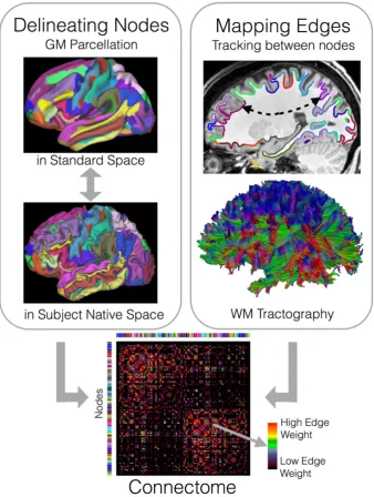
Inferring amacro‐connectome from dMRI images is a very challenging task and a field of active research. We divide connectome mapping into
two tasks: node delineation and edge mapping (Figure 1). Nodes represent spatially distinct cortical and subcortical gray matter regions, while edges
represent the white matter fiber bundles that interconnect pairs of regions.
2.1
|Node delineation
Specifying a parcellation scheme that subdivides cortical and subcortical gray matter into discrete, spatially contiguous parcels is not
straightfor-ward.28Architectonic atlases provide the simplest and perhaps most commonly used approach. Many such atlases are available (see Reference29
for a review) and they can be registered to an individual brain to ensure that nodes between subjects are matched with respect to average size,
geometry and location. However, architectonic and other template‐based atlases do not capture variation between individuals in regional
func-tional boundaries and thus make the simplifying assumption that a common parcellation is representative of all individuals. For instance, the
AAL30and Harvard
‐Oxford31atlases are based on anatomical landmarks, while the parcellation of the Talairach Daemon32and the Juelich atlas33 are based on cytoarchitectonic features from post‐mortem brains.
Data‐driven parcellations offer an individually customized alternative. Data from task‐based or resting‐state functional MRI can be used to
define areas with homogeneous features across a population comprising hundreds of subjects.34-38In this way, regions are delineated based on
functional properties that are specific to the individuals for whom connectomes are to be mapped. Methods for defining functional boundaries
are many and varied, with the most recent utilizing multiple modalities and unique measurements. For instance, Reference39uses multiple features
simultaneously, such as cortical folding, myelin content and resting‐state and task‐based activity, to identify a functionally relevant and population‐
specific parcellation, which respects individual variability. In Reference40, the authors use structural, functional and behavioral features to identify a
parcellation consistent across various domains.
2.1.1
|Limitations and open problems
dMRI and tractography methods can be also used to extract connection patterns and probe functional boundaries.4,9This has been shown with
controlled studies for a large number of regions in the cortex and subcortex (for instance References41-44; see also Section 3.2). However, current
limitations in structural connectome estimation, as we explore throughout this review, can limit the accuracy, interpretability and generalizability of
such approaches for node delineation.
While parcellating the cortex based on functional homogeneity is an attractive alternative to node delineation, it also suffers from
methodo-logical caveats.45Furthermore, a number of conceptual problems exist with respect to the definition of areal boundaries.46Here, we briefly review
some of these considerations.
*Extrinsic4,9
connections that traverse white matter include local U‐fibers (up to ~30 mm in length) connecting neighboring regions and long‐range fascicles connecting remote regions within or between hemispheres. Intrinsic connections are horizontal and intra‐cortical (<3 mm in length). It is estimated that the number of intrinsic connections (~1011
fibers) is an order of magnitude larger than the number of U‐fibers (~1010
). The number of U‐fibers is an order of magnitude larger than the number of long‐range connections (~109
fibers).26
Individual variability
Individual variability in brain function and structure complicates the interpretability of population‐level parcellations. Well‐characterized areas, such
as V1, can vary twofold in areal size across subjects.46,47The relationship between functional boundaries and cortical folding is also highly variable.
Areas associated with high‐order function exhibit more variability across subjects in folding patterns than primary areas, where the folds can be
reasonable predictors of the boundaries.48Therefore, a group
‐level parcellation template cannot capture subtle yet important variations between individuals. Registration frameworks that align functional features rather than simply matching geometry or cortical folding could offer a way to
approach this problem.49
Within‐region heterogeneity
Different patterns can characterize the functional and topographical organization of a region. For instance, different within‐area topographical
organizations can underlie different functions of the same region.50V1 and V2 provide such examples, with their central and peripheral
subre-gions exhibiting different relationships with other resubre-gions of the cortex.46This within‐area heterogeneity, along with individual variability, makes
delineation of boundaries very challenging. A potential solution is to define smooth transitions and fuzzy boundaries between regions rather
than binary parcellations. However, this fuzziness should reflect uncertainty in functional features rather than data noise, folding differences
[image:3.595.129.468.52.501.2]or alignment errors.
Scale and number of nodes
In many studies, the coarseness of gray matter subdivisions is a relatively arbitrary choice. Principled data‐driven methods to perform model
selec-tion and define an optimal number of nodes exist for parcellaselec-tions based on funcselec-tional data.37However, these methods may be conflicted by the
trade‐off between true functional relevance and discriminative power of the available data. For instance, using fMRI versus MEG data is
accompa-nied by different limitations in spatial and temporal resolution, which can influence model selection. For this reason, some investigators have
resorted to multi‐scale schemes to ensure findings are generalizable and not sensitive to a given parcellation resolution.51,52
The coarseness of a node parcellation influences the process of mapping white matter connections. In practice, edge mapping and node
delin-eation are performed independently and the outputs of these two processes are only combined when mapping a connectivity matrix. Parcellations
with fewer regions tend to give more reproducible and“smooth”mappings than finer ones, whereas more detailed parcellations in principle
pre-serve more details.53,54Low
‐to mid‐scale parcellations (of the order of tens to a few hundred regions) have been shown to increase agreement of dMRI‐estimated connectomes with tracers in the mouse55,56and monkey brain57when compared with results from finer subdivisions.
In summary, methods for delineating connectome nodes are many and varied. The number of nodes and specific nodal parcellation that are
best suited to a given application are usually not obvious. Parcellations that are informed by brain anatomy and/or functional specialization have
gained significant traction in the field. In the future, parcellation strategies should be developed that capture individual variability. Unlike the
micro-scale, where the parallel between nodes and neurons is obvious, defining nodes at the macroscale is less clear. It is therefore important to assess
the consistency of results for a coarse anatomical parcellation as well as a finer parcellation that is delineated functionally or perhaps randomly.
Inconsistencies that emerge between these two scales can potentially shed light on the nature of a particular finding.
2.2
|Mapping edges
Once the nodes of a connectome have been defined, tractography can be used to estimate edges—the connecting paths between pairs of regions.
While other indirect methods exist,17,58dMRI
‐based tractography is the only method that allows localization of white matter bundlesin vivo(see References59,60and papers in this special issue for reviews). Axonal fiber bundles are organized coherently such that water diffusion occurs
pref-erentially along the orientations of least hindrance, which are typically parallel to the fibers. In contrast, diffusion is maximally hindered in the
per-pendicular direction. The preferred diffusion orientations (PDOs) can be indirectly mapped to fiber orientations at a voxel‐wise level (see
References61,62and papers in this special issue for reviews). Tractography approaches then integrate the voxel
‐wise information at a global scale and propagate curves that are maximally tangential to the local PDOs.63These curves provide estimates of the white matter bundles.64
There are a plethora of methods for mapping fiber orientations and for curve propagation. The diffusion tensor model65is the simplest
approach and provides a unimodal approximation to the underlying fiber configurations. A more accurate model in the case of complex fiber patterns
is the fiber orientation density function (fODF), which characterizes the fiber distribution in each voxel. Deconvolution methods, parametric42,66-68
or non‐parametric,69-71q‐ball imaging72and diffusion spectrum imaging73are some of the popular methods that can provide estimates of the fODF†
and a discrete number of crossing orientations in each voxel. The importance in estimating crossings and the maturity of deconvolution methods
have been shown in many instances for tracking deep white matter‡(e.g. References73-78). A recent study showed benefits of considering fODFs
for tracking into the transition from white matter to gray matter.79
Tractography methods can be grouped into two categories: (i) local approaches,63,80-82which in a greedy, step‐by‐step fashion propagate
curves (or streamlines) that are tangent to vector fields extracted from the fODFs; (ii) global methods (for instance References83-89), which estimate
paths that are optimal according to a global criterion. Such paths are not necessarily tangent at every point of their route to the local fODF/vector
fields. In principle, they are less susceptible to local errors. Local methods have been by far the most popular and applied approaches. Global
methods offer a promising alternative,77,90but they require further validation, and they can be more cumbersome and computationally demanding.
Global methods have been tested mostly for deep white matter tracking, and thus the extent to which they share or solve the limitations inherent
to local methods (see next section) is yet to be explored.
Local streamline methods can be further subdivided into deterministic and probabilistic, depending on whether they perform a deterministic or
stochastic estimation. Deterministic methods63,81provide a point estimate of the path of least hindrance to diffusion between two points.
Prob-abilistic methods42,82estimate a spatial distribution for this path. They estimate the uncertainty around the local fODF peaks (through parametric
or non‐parametric inference)42,82,91and account for this uncertainty to obtain the path distribution (peak‐based probabilistic methods). A variant of
these approaches uses samples from the whole fODF to obtain the distribution (whole‐fODF probabilistic methods; see Jeurissen et al92for an
illustration of this difference).
Several studies have evaluated the test–retest reliability of these methods for connectome reconstruction.93-95Estimates derived from
prob-abilistic tractography generally show greater connectome reproducibility than deterministic methods, reduce the effect of residual spatial
misalign-ment errors and potentially improve some of the statistical properties of the sampled paths (i.e. normality). At the same time, they can be to the
†Strictly speaking,q‐ball and diffusion spectrum imaging provide an estimate of the diffusion ODF, a blurred version of the fODF.
‡We use the term“deep white matter”to denote all white matter under the white‐gray matter boundary. This is in contrast to white matter at the boundary and above,
detriment of connectome specificity and accuracy.96Probabilistic tractography yields greater spatial dispersion in streamline trajectories, which
may lead to more spurious connections (particularly for whole‐fODF sampling methods97). On the other hand, connectomes derived from
deter-ministic tractography generally comprise fewer connections, but results show substantially greater variation within and across individuals
(partic-ularly in data with low angular resolution or low signal‐to‐noise ratio (SNR)). It is unclear what proportion of this variation represents genuine
anatomical variation between individuals, as opposed to noise due to a poor fitting local fiber orientation model, tractography errors or residual
misalignment between the streamlines and regional brain atlas.
The seeding strategy also has an effect on finding the edges of a connectome.98Streamlines are typically initiated from all white matter and the
streamlines intersecting pairs of nodes are mapped to the respective edge.8This“brute force”approach was originally suggested to be more
sen-sitive to the detection of long white matter bundles.99An alternative is to seed from the boundary between white and gray matter.100,101Boundary
seeding has been recently shown to provide smaller biases of dMRI estimates when compared with biological ground truths (for instance less gyral
bias, better predictions of path length distributions, slightly better sensitivity versus specificity performance).23,102
2.2.1
|Limitations and open problems
Diffusion‐to‐axon mapping is ill posed
Finding connections is based on a mapping from water diffusion to fiber orientations, which is inevitably required due to the indirect nature of
dMRI. Such inference is in general an ill‐posed problem,60,61but the problem becomes identifiable using approximations and assumptions.
Improv-ing data quality and estimation methods to reduce potential errors arisImprov-ing from these assumptions has therefore been at the heart of dMRI
research.
MRI voxels (even at high resolution) are too large to enable the resolution of axons. Thousands of axons coexist within the volume occupied by
an imaging voxel. The measured macroscopic signal is therefore considerably far from the scale of interest. As a result, different ground‐truth fiber
patterns can lead to very similar signal profiles within a voxel. An example is shown in Figure 2A. Voxel‐wise fODF estimation does not have the
information to differentiate between these patterns, as they correspond to similar signal profiles. The current approaches rely on approximations
and typically assume that patterns with fiber orientation dispersion provide evidence for crossing fibers. Looking for and using discrete local
max-ima in these fODFs (when in reality there is a fanning or a sharp bending pattern) can lead to false positives and negatives.60Efforts have been
made to extract continuous features (other than the maxima) from the fODF and go beyond crossing fibers.66,103-106However, taking advantage
of this information in tractography is not straightforward and only recent frameworks explore such integration.109,110,112
Another factor that compounds the difficulty in identifying local fiber orientations is the axial symmetry of the diffusion signal. Diffusion in
opposing directions will give rise to the same measurement. As a result, voxel‐wise fODF estimates are antipodally symmetric as well, even if the
ground‐truth patterns are not. Figure 2B,C shows the errors caused by ignoring this asymmetry when tracking diverging and converging bundles.
These inherent limitations make tractography methods very prone to errors. Imposing anatomical constraints56,101and/or tractography
filter-ing107,108offers ways to reduce false connections in principle. However, these do not solve the problem of missing connections (false negatives),
and caution is needed as filtering can generate spurious between‐group differences due to the effective re‐distribution of streamlines. These
lim-itations highlight the need for new paradigms. For instance, inferring asymmetric fODFs is possible by considering neighborhoods of voxels rather
than individual voxels.109-112Augmenting tracking with microstructure113-116offers a more robust alternative to orientation‐based tracking, as
esti-mated bundles have structural features preserved along their route rather than orientation alone.
Finding terminations is inherently limited
Mapping a connectome demands accurate fiber tracking in deep white matter as well as accurate determination of fiber termination points in grey
matter. Identifying fiber termination is inherently difficult with tractography.60In fact, tractography cannot terminate propagation in an
unsuper-vised manner and heuristics need to be used to determine endpoints. This makes termination criteria an important choice and is the reason why
anatomically driven rules can improve reliability of results.100,101For instance, crossing the white/gray matter boundary (WGB) multiple times is
likely to yield spurious trajectories, and propagation within the cortex may be prone to greater errors due to low anisotropy in grey matter.
Recovering laminar organization of connectivity is an example where finding terminations with current dMRI technology is impossible.
Differ-ent layers in the cortex may preferDiffer-entially connect to differDiffer-ent regions.17,117Layer
‐specific orientation information has been shown with extremely high spatial resolution imaging ofex vivotissue.118However, even if this information was availablein vivo(for instance with some variant of the
approach proposed by Barazany et al119), termination points to different layers would not be estimable using tractography,60as the algorithms
are insensitive to synaptic endpoints. Similar problems exist with subcortical/cerebellar nuclei, within which tractography cannot find synaptic
ter-mination locations. A difference, however, is that the inherently higher anisotropywithinmajor subcortical structures allows topographical
organi-zation and connection patterns to be probed within their volumes (for instance see References42,120or Figure S3 in Glasser et al121). In the case of
cortex, due to low anisotropy, contrast and the inherent resolution limits, we are mostly sensitive to connectional patternsalongthe cortical sheet
(WGB) (see Section 3.2 for examples).
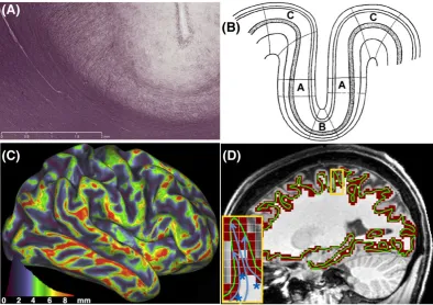
In the cortex, another obstacle that biases the estimation of termination points is the presence of superficial white matter fibers, such as the U‐
fibers that run parallel to the WGB122(see myelin‐stained fibers at a sulcal fundus in Figure 3A). The density of these fibers is higher at the sulcal
the boundary and escape white matter. This under‐representation of tractography streamlines at the sulci compared with gyri was first described
by Van Essen et al27asgyral bias. This bias is expected to be more evident for finer parcellation schemes and a large number of nodes, yet it can
potentially introduce a confound for coarser parcellations as well, particularly when average curvature and sulcal depth profiles vary considerably
across nodes.
2.3
|Quantifying edges
As described above, tractography can provide an estimate of the trajectories representing fiber bundles. Ideally, a connectome should also include
estimates of connection strengths (for instance axonal densities, myelination, diameter). dMRI cannot provide such direct measures,25,60but allows
estimation of edge weights that indirectly reflect some of these properties of interest. These range from simple binary values, denoting the
pres-ence or abspres-ence of an edge, to approximations of biophysical properties of connections, reflecting micro‐or macro‐structure.
Connection strength is most typically quantified using some function ofstreamline counts, the number of streamlines intersecting a pair of
regions. Streamline counts can be enumerated for all pairs of regions to populate the cells of a connectivity matrix.7,8Streamlines that are permitted
[image:6.595.100.499.50.473.2]pairs. Anatomical constraints can be imposed to avoid such scenarios, which terminate streamlines either at the white/gray matter interface or
within subcortical volumes.101
Streamline counts can be symmetrized, normalized or transformed in various (nonlinear) ways,85which aim to reduce the effect of confounds
reflecting algorithmic choices and ensure better consistency across subjects. Power transforms, in particular the logarithm, can be applied to the
streamline counts before analysis to achieve normality. Normalization by node sizes8,123can be used to account for volume/area variability in
the chosen gray matter parcellation. While it may be that larger brain regions are indeed more strongly connected by virtue of anatomy, a greater
number of streamlines is likely to terminate in regions with a larger interface between grey and white matter due to the tractography process.53,100
Normalization by row and column sums of the matrix, such as fractional scaling, provide enhanced relative contrast of a particular edge to the rest
of the edges that involve any of the two connecting nodes and improves the power to predict tracer‐measured connection strengths using
tractography‐derived weights.23
Diffusion path probabilities, obtained from probabilistic tractography, reflect normalized conditionals of streamline counts given the
orien-tation model, seeding strategy and termination/counting criteria.74,82As discussed before, due to the stochastic generation of streamlines,
probabilistic tracking provides a spatial distribution on the path of least hindrance to diffusion. The relative contrast of path probabilities have
been recently shown to correlate with connection strength measured using tracers,23similar to deterministic streamline counts.124However,
path probabilities are also confounded by many uninteresting factors (such as path geometry, noise, modeling errors), which make direct
inter-pretations difficult.25,60
Alternative metrics that reflectmicrostructuralproperties along edges can be considered as edge weights. For instance, voxel‐specific measures
of anisotropy can be averaged over all voxels traversed by a path that is assigned to a particular pair of nodes.125The resulting tract
‐averaged mea-sure thus characterizes the anisotropy of a connectome edge as a whole. Other microstructural meamea-sures can be also used,125,126such as axonal
myelin content measures derived from images of magnetization transfer ratio.127,128Different weighting functions can be employed for the
aver-aging process to give greater weight to different parts of the tract (e.g., using streamline counts/probabilities in each voxel can give greater weight
[image:7.595.100.495.49.327.2]in the main tract core versus the periphery).
Features that reflect tractmacrostructureare another possibility for edge quantification. In fact, volume and cross‐sectional area of paths
intu-itively relate more directly to connection strength than their microstructure counterparts. Close et al129use explicitly the tract volume in a model to
parameterize connection paths using spatial basis functions. Extensive simulations illustrate the potential to infer volume as a probe of apparent
connection strength, but high computational demands currently limit exploration, and utility in real data is yet to be shown. Smith et al108present
a post‐processing filter of streamlines based on a generative model of the data from streamlines (similar in spirit to References107,130). The filtered
streamline counts are proposed as probes of the cross‐sectional area of the white matter connection underlying an edge. Even if such an
interpre-tation is based on the assumption that relative fODF volume fractions reflect relative axonal densities, the filtering increases the biological
rele-vance of the obtained edge weights.102
2.3.1
|Limitations and open problems
The major limitation for quantifying edges is that none of the above approaches provide directly an inter‐regional measure of the number of
connecting axons, which is a desirable measure of connectivity strength in typical neuroanatomy applications. Tract‐averaged microstructural
mea-sures may provide an interpretable biophysical property per edge. However, it is questionable how informative such properties are when treating
connectomes as networks, which would require some proxy of connectivity. In a recent study no correlation was found between such microstructural
measures and axonal strengths measured by tracers.124On the other hand, functions of streamline counts can be thought to be more relevant in such a
network context.23However, factors that reflect data quality, algorithmic choices and inherent limitations bias these measures,60as we discuss below.
Future work should also focus on characterizing the distributional and noise properties of connectivity matrices. Connectivity matrices
com-prising streamline counts derived from probabilistic tractography are likely to show smoother variations between spatially neighboring node pairs
compared with deterministic tractography, as streamline trajectories associated with probabilistic tractography are more spatially dispersed.
Distance bias
Streamline counts between distant regions, interconnected by longer tracts, are often smaller than counts between neighboring regions.
Algorith-mic limitations contribute to this pattern; for instance, longer tracts are more difficult to reconstruct with tractography because streamlines must be
propagated for a longer distance and each propagation step provides an opportunity for“wrong turns”.131,132However, connection strengths as
measured by tracers follow an exponential decay with connection length, with the majority of connections being short and strong and the long
connections being weak, comprising fewer axons.133,134Tracers of course have their own error sources,17but the extent to which the algorithmic
distance bias of tractography is biologically specific remains to be explored.
Seeding bias
When streamlines are seeded from all of white matter, longer tracts are inevitably sampled more abundantly because they occupy a greater volume
than shorter tracts. To compensate for this bias towards long tracts, the streamline count can be normalized by the average length of the
stream-lines contributing to the count.135However, given that many tracts are sheet
‐like and vary considerably in cross‐sectional area and morphology, simple normalization factors such as the streamline length might not adequately correct for the over‐sampling of tracts occupying greater volumes.
Filtering of streamlines via generative models that ensure higher fidelity with the data107,108,130is another approach that seems to be more
ben-eficial in this context. Initiating streamlines from the WGB interface is an alternative that overcomes this limitation and can potentially provide
more realistic path length distribution,23,100,102but this seeding approach has difficulty in tracing out long fiber bundles.
Gyral bias
As described in the previous section, the existence of superficial tangential white matter can lead to under‐representation of tractography
stream-lines at the sulci compared with gyri,122the so
‐called gyral bias.27The bias is further magnified by algorithmic limitations in tractography; sharp turns (needed to capture axons, which can bend at quasi‐right angles15) are less preferred than linear trajectories that will lead most of the time
to the gyral crowns.
The gyral bias is biologically relevant. The preferential termination of tractography streamlines at gyral crowns agrees with neuro‐anatomical
expectations. It is the tractography‐predicted magnitude of the difference for preference towards gyral crowns compared with sulcal fundi that is
unrealistic.27Indeed, let us postulate that the number of axons crossing the WGB is constant per unit cortical volume (as we have no evidence to
assume otherwise). Cortical folding however induces geometrical differences in different parts of the cortex. Cortex tends to be thickest along gyral
crowns and thinnest in sulcal fundi136(Figure 3B), and larger cortical volume corresponds to a unit surface area of the WGB at the crown compared
with the fundus. Therefore, even if the number of axons crossing the WGB boundary is roughly the same per unit volume of cortex, the density of
axons per unit surface crossing at the gyral crowns will be larger compared with the axon density crossing at the sulcal fundi. Van Essen et al. used
cortical thickness measures to compute this expected bias (Figure 3C) and found that it is four to five times less than that predicted by tractography.27
New paradigms are needed to address these limitations when tracking close to the WGB. Some very recent studies have taken preliminary
steps in this direction. Cottaar et al137explore the relationship of fiber orientations to cortical features using post
‐mortem high‐resolution his-tology to inform generative models forin vivodMRI. St‐Onge et al138impose a strong prior on the fiber orientations within the cortical ribbon
tracking, such as those used before for deep white matter,110may also be beneficial for improved estimates of the transition between white and
gray matter.
Surfaces or volumes?
Boundaries, such as the WGB, can be represented either as volumes or as surface meshes. Surface representations offer a more compact and
accu-rate description of the boundaries at a given resolution.139This can have an effect on the tractography results and their interpretation. For instance,
an intermediate‐resolution, voxel‐based representation of the WGB cannot necessarily follow the highly convoluted boundary (Figure 3D) and can
mask the gyral bias. As shown in the inset of Figure 3D, the streamlines are frequently unable to reach a voxel representing the gyral crown without
first traversing a voxel that represents the sulcal fundus. Depending on the width of a gyrus and on how tractography boundary conditions are
imposed, this can artificially increase the visitation frequency to certain sulcal regions (blue asterisks in Figure 3D). However, these frequencies
and their spatial pattern may purely reflect resolution‐induced limitations of the voxel‐wise representation. Using surface meshes, such as GIFTI
files,139should be more robust to these problems, but the exact differences between results obtained from the two representations remain to
be explored.
Summary
The reconstruction and mapping of connectome edges is confounded by many limitations and open problems remain to be solved. Reproducible,
sensitive and specific measures of white matter connectivity are difficult to obtain with dMRI. Despite these limitations, dMRI enables
reconstruc-tion of connectomes, which display biological properties that are consistent with brain networks mapped with alternative modalities. Recent
stud-ies explore this directly,23,102,124while a plethora of studies provide indirect evidence in favor of consistency between modalities. We review this
evidence in detail in Section 3.
2.4
|Impact of data quality
So far we have discussed the impact of algorithmic and methodological choices on building connectomes. Another important aspect that affects
estimation of dMRI‐derived quantities in general (and therefore connectomes) is data quality. Given the inherent limitations of dMRI, better data
can help if developments allow: (i) improvements in diffusion‐to‐axon mapping and (ii) reduction in partial volume. SNR, spatial resolution, angular
resolution and angular contrast are some of the data features that can directly influence these factors.28Even if some limitations cannot be directly
overcome with better data (see Reveley et al122and some of the conceptual problems described in the previous sections), significant improvements
in tracking white matter have been shown.
More specifically, better SNR and/or angular resolution improve precision and accuracy of the mapping from diffusion signal to fiber
orienta-tion estimates.140Improved angular contrast allows higher sensitivity in detecting within
‐voxel complex fiber patterns,69,73,76which further allows more accurate tractography.74Multiple angular contrasts (i.e.bvalues) give better estimation of partial volume and differentiation of diffusion
com-partments and further augment accuracy of orientation estimates.141,142
Increased spatial resolution reduces partial volume and allows imaging of exquisite details of white matter organization.143-145For instance,
very high‐resolution dMRI allowed the mapping of axonal and dendritic networks in the hippocampus, whose accuracy was confirmed with tracers.
High spatial resolution is also beneficial for better distinguishing tract termination points.146Increasing the resolution by using high field strength
improves the estimation of the fiber spreading pattern to the cortex and reduces gyral bias.147In another recent study, improving on all the data
quality aspects of dMRI data increased agreement of connectomes estimated in humans using three different modalities.148
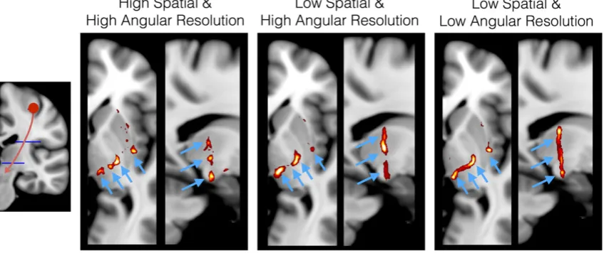
In Figure 4, we illustrate a simple example of how changing spatial and angular resolution of the data affects tractography. In this particular
case, the increased spatial resolution is beneficial in differentiating thin projections from the hand area of the motor cortex. Apart from better
resolving partial volume, higher spatial resolution is expected to increase the estimation accuracy of relatively short paths, which comprise the
majority of brain connections.19,133It is important to note, however, that increasing spatial resolution at the expense of contrast‐to‐noise ratio
or angular resolution can actually lead to suboptimal performance,146,150particularly in tracking major bundles.
Deciding on the acquisition protocol and getting the balance of these features right is governed by a series of trade‐offs (for instance SNR
com-peting against spatial resolution or angular contrast). As shown in Figure 4, it may not be optimal if a feature is improved at the expense of others.
Recent frameworks attempt to resolve these trade‐offs by fusing complementary datasets (e.g. data with high spatial and low angular resolution
with data with low spatial and high angular resolution).147,151Another group of post
‐processing methods boost certain features to improve esti-mation. These include denoising approaches for improving SNR152,153and up‐sampling or super‐resolution methods for improving spatial/angular
resolution.154-156Nevertheless, we can expect recent technological advances to provide better operating points for all these competing features
and improve overall data quality. Hardware developments in modern scanners,157such as higher gradient strengths, can translate to improvements
in SNR and contrast of routine scans. While higher field strengths might pose difficulties to dMRI acquisitions due to the shorterT2relaxation times
at high field,157they can be used to achieve very high spatial resolution.143,158
Sequence developments should accompany these hardware advances. For instance, simultaneous multislice or multiband acquisitions159,160
allow three‐to fivefold acceleration of dMRI scan time, changing the perception of the data quality that can be achieved in realistic time frames.
gradients (see Shemesh et al161for a review) or generalized trajectory imaging162open new possibilities in probing restricted compartments and
microscopic features with the potential to improve the accuracy of mapping from diffusion measurements to tissue structure.
Better data enable improved modeling and analysis.60In fact, new tools are required to take full advantage of the new information in certain
applications. An example is increasing spatial resolution in the presence of inevitable subject motion and eddy currents. The higher the resolution,
the higher the need is for accuracy in distortion correction tools. New frameworks in this area163,164have been shown to limit alignment errors
between dMRI volumes to less than a quarter of the voxel size165and improve distortion correction,166hence preserving the benefits of high‐
res-olution acquisitions after preprocessing.
3
|V A L I D A T I O N A N D C O M P A R I S O N W I T H O T H E R M O D A L I T I E S
We have highlighted a series of limitations for mapping the connectome using dMRI. It is therefore important to quantify the effect of these
lim-itations on the ability to accurately map connectomes. It is also important to explore the utility and biological consistency of current connectome
mappings given the limitations of dMRI and tractography and that an increasing number of frameworks are being developed with this aim (e.g.
References78,97,167-169).
In the following sections we review studies that specifically compare tractography‐induced estimates with estimates from other modalities;
either directly for the purpose of validation or indirectly for the purpose of multi‐modal integration. The comparisons show differences (and
limi-tations as highlighted in the previous sections), but also provide evidence of agreement and predictive power in various different contexts that are
greater than expected due to chance.
3.1
|Direct evidence
There have been efforts to directly validate parts and aspects of the tractography‐estimated connectome with different invasive modalities, such as
chemical tracers, primarily in animals. Tracers have their own limitations and biases.17For instance, identifying correspondence between injection
sites and a particular brain area is not straightforward. Axons that traverse the injection site can result in the reconstruction of spurious connections
because these axons can absorb the tracer even though they make no synaptic contacts with the injection site (particularly in the rat brain, where
fibers can bifurcate in gray matter). Absolute quantification of connection strength is also difficult, as anterograde and retrograde tracers depict
different features of connectivity. However, tracers are very precise in spatial localization and have a considerably lower false positive rate than
tractography. Thus, even if not perfect ground truths, they are much closer to the ground truth thanin vivodMRI.
Validation efforts have focused on the ability of tractography to estimate the existence of edges (and the route of underlying connections), as well
[image:10.595.87.511.53.231.2]the following. (i) Tractography predictions are above chance; however, features with poor agreement exist. (ii) There is a trade‐off between sensitivity
and specificity. Tractography methods that tend to be more sensitive in finding connections are also less specific. (iii) Cortico‐subcortical, short‐range
intra‐hemispheric and homotopic inter‐hemispheric connections are more reliably estimated. (iv) Weights estimated by tractography provide a
reason-able estimation of connectivity strength for some pairs of regions. (v) Parcellated connectomes, i.e. those estimated with nodes corresponding to mid‐
scale regions, are more accurate than denser ones that attempt to depict fine, within‐region, details. In the following paragraphs we review the
rele-vant studies and findings in more detail.
3.1.1
|Identifying connection trajectories
The first validation studies investigated how well tractography can identify large bundles and follow them through white matter. Qualitative
com-parisons have shown good agreement against histological tracing in the monkey brain170or against dissected human samples.171,172Newer
dissec-tion methods173allow preservation of the cortex and of the superficial white matter and have shown examples of the ability of tractography to
follow the true route of connections up to their terminations.174,175However, semi‐quantitative comparisons have also highlighted false positive
connections that are estimated.176,177
The sensitivity (finding true connections) and specificity (avoiding false connections) of tractography in detecting connectome edges has been
more systematically explored in comparison to chemical tract tracing in the monkey,23,90,178,179mouse55,56or porcine brain.180Areas under the curve
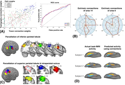
in receiver‐operating characteristic (ROC) plots have been reported in the range of 0.7 to 0.8, suggesting a fair estimation accuracy in identifying
con-nections and/or their routes (Figure 5A). At the same time, all studies illustrate the strong dependence of the results on the particular tractography
set-tings and models. Probabilistic tractography is less sensitive than deterministic to anisotropy and curvature thresholds or the tissue composition of the
seed.178,179It also tends to be more sensitive, but less specific, than deterministic methods and more susceptible to false positives.97,178,180In general,
an increase in sensitivity for all methods comes at the expense of a decrease in specificity, and therefore an optimized set of parameters is important.
Also, tractography performs much better when exploring connections between relatively large cortical nodes rather than fine details within regions.
Comparisons of dMRI‐estimated paths with tracers also reveal benefits of considering fiber crossings in tracking (larger benefits are shown in
some cases180than in others178). Adding prior knowledge to guide connectome mapping is also beneficial.56In Jbabdi et al181, organizational
princi-ples of cortical projections identified with tracers were found and generalized to post‐mortem macaque MRI data using informed tractography
pro-tocols that includeda priorispecified waypoint and exclusion masks. These were then used to search for and identify similar principles in humans. In
Draganski et al182, subcortical connectivity signatures were obtained and revealed a series of networks between basal ganglia sub‐nuclei and the
cor-tex. Some of these networks, in particular cortico‐striatal circuits, were directly validated against previous tracing studies in monkeys.
3.1.2
|Tractography
‐
estimated weights
An even more challenging task than localizing connections is extracting relative weights for the connectome edges. The recent development of
comprehensive and weighted brain mappings by collating a plethora of tracing experiments19,20 has permitted direct comparison with
tractography‐derived connectomes. From these studies, we can extract some general features of the connectivity weights as measured by tracers:
(i) There is a wide range of connectivity strengths than spans five orders of magnitude. (ii) An exponential reduction of connectivity strength occurs
with path length.133,134(iii) There is a prevalence of local connections. Short connections are significantly more common and significantly stronger
than long connections.
In one of the most recent comparisons, the authors evaluated the accuracy of dMRI connectomes in predicting generic features extracted from
human brain dissections.102The connectome edges and weights correctly replicated the relative percentage of long inter‐hemispheric and intra‐
hemispheric connections and the inverse relationship between connection strength and length.
Non‐human primate studies allow more detailed comparisons due to the plethora of available ground truth. Donahue et al23compared the
connectome edges and weights obtained via macaque tractography and macaque tracers. Tractography could recover four out of the five orders
of magnitude in the range of connection strengths. The performance was far from perfect, yet better than chance, even for the weakest of long
paths (Figure 5A). Strong and short connections were better characterized by tractography, as the performance worsens with smaller connection
weights. Overall a correlation of about 0.55§was reported between edge weights in tracer and tractography, and the path length dependence
con-tributed significantly to this correlation. Interestingly, however, after regressing out path lengths, there was still a significant correlation (but smaller
~0.25) between the two measures, showing that it is not only the path length dependence that drives the relationship. Similar trends were reported
by Van den Heuvel124(though with smaller overall correlations, ~0.35, and a different definition of connectome weights, focusing on absolute
streamline counts rather than relative contrasts of weights).
The dependence of these correlations to the node size was explored in References55,56and for the mouse brain. Connection weights between
mid‐level sized regions were more reliable (correlation up to 0.77 in Calabrese56) compared with considering small nodes (correlation dropped to
0.45). Comparable correlations were observed for the monkey brain.57As discussed in the previous sections, certain limitations reduce the
reliabil-ity of tractography at finer scales. Despite the errors, all the validation studies provide evidence that dMRI‐induced connectomes contain relevant
§
To put these correlation values into perspective, comparisons between histology and MRI‐derived values of a much more straightforward feature, such as cortical
thickness, give correlations of the order of 0.6–0.7,183,184
information and predictive power. Interpretation might not always be straightforward, but a large number of applications show that this
informa-tion can be useful. We review some of these applicainforma-tions in the following secinforma-tion.
3.2
|Indirect evidence
The idea of connectivity fingerprinting using tractography weights (Figure 5B)4has been applied to identify boundaries of functionally distinct
regions (see References45,185for reviews). In one of the earliest studies,43a dense weighted matrix mapping connections from the medial frontal
cortex to the rest of the brain was obtained using tractography. This matrix was used to identify the boundary between the anterior and posterior
parts of the supplementary motor area. These are functionally distinct areas in both motor and cognitive domains, and the boundary, identified as a
sharp change in the tractography profiles, agreed well with that obtained from functional MRI localizer tasks. Since then, similar results in predicting
functional boundaries using dMRI and agreement with functional MRI have been shown for various cortical41,44,186-192and subcortical areas 42,193-195
(see Figure 5C). Agreements have been also illustrated with other non‐MRI functional measurements, including PET120and direct
electrophys-iological recordings,196as well as cytoarchitectonic delineations.197,198
Tractography“signatures”are reproducible and robust across subjects to a degree that allows predictions for the efficacy of targets in
func-tional neurosurgery.199,200In deep brain stimulation, neurosurgeons search for the most efficient stimulation target via trial and error. Pouratian
et al201identified in this classical way the thalamic location that when targeted for stimulation allowed the most efficient alleviation of tremor
[image:12.595.48.548.48.390.2]surgery and the thalamic region best matching this fingerprint was identified and used as the initial target for stimulation. They found that in these
new patients the tractography‐informed target was indeed very close to the most efficacious location, allowing better surgical planning.
The functional relevance of structural connectomes has been further illustrated by studies that use structure to constrain or predict function
(Figure 5D). Models of functional networks built on a structural backbone have increased explanatory power and identifiability compared with
models that lack such structure.202,203Structural connectivity networks alone have been used to predict the existence, strength and spatial features
of functional connections as assessed by fMRI at rest.204During a task, the functional activation maps have been predicted solely by the
connec-tion pattern of the activated region.5More specifically, Saygin et al5learnt a model in a group of subjects between the tractography
‐estimated connectome of the fusiform gyrus and the functional activity recorded via fMRI during a face selection task. They then applied that model to
the connectome of new subjects and predicted their task activation. This predicted activation was found to be very similar to the activation
indi-vidually measured by subsequent fMRI. A subsequent study used a similar mapping approach and predicted the functional organization in young
children after they learnt how to read, using the structural connection patterns they had developed prior to acquiring this skill (i.e. a few years
ear-lier in their development).205Such structure–function relationships can be observed even at a higher level, with structural connections predicting
behavior and decision‐making processes.206-208
Mapping connection patterns offers the unique ability to perform comparative anatomy (see Mars et al209for a review). This allows the
iden-tification of“homologue”areas across species (areas that share similar“connectivity contrast”) and the translation of the vast literature of animal
studies to humans,210-213but also translation from humans to other primates to study evolution.214-217Such studies provide evidence of
agree-ment of the structural estimates with a large range of independent sources of information.
4
|N E T W O R K A N A L Y S I S
Connectivity fingerprinting approaches discussed in the previous section (Figure 5B,C) mostly reflect hypothesis‐driven analyses, where a subset of
the connectome is considered and relative connection patterns associated with certain nodes are examined. An alternative approach considers
net-work properties, either in a data‐driven manner or with respect to hypothesis‐driven regions. Complex networks have been studied in mathematics
for centuries, where they are known as graphs and are fully defined by their nodes and edges (Figures 1 and 6). In this section, we consider how
graph theory and network science can be used to understand the global organization of the connectome.
The edges of a graph are either directed or undirected. Edges inferred from tractography are invariably undirected because the direction of
diffusion cannot be resolved with dMRI (in contrast to tract tracing methods, which can distinguish between afferent and efferent fibers).
Further-more, the edges of the graph can be either weighted or binary, as previously discussed.
4.1
|Adjusting density and weights
Thresholding methods applied to brain graphs with weighted edges reduce the density of connections in a graph and aim to eliminate spurious
edges, thus improving specificity. Thresholding can be further applied to binarize graphs221,222and simplify the interpretability of certain analyses
by emphasizing network properties that may be obscured by large variations in edge weights. On the other hand, thresholding may disregard useful
information (see previous section and representative examples in References5,43,206). Therefore, the applicability of such approaches depends on
the particular question of interest.
The simplest thresholding method, calledweight‐based thresholding,involves eliminating any edges with a weight that is below a given global
threshold. To yield a binary graph, the weights associated with the remaining edges are disregarded, leaving only information about whether edges
are absent (0 in connectivity matrix) or present (1 in connectivity matrix). Weight‐based thresholding introduces the confound of graph density to
comparisons between groups of individuals. Graph density¶—the proportion of all node pairs that are directly interconnected by an edge—
funda-mentally influences the properties of a graph.222Applying the same global threshold to different brain graphs does not necessarily ensure that the
resulting thresholded graphs have the same density. Therefore, when complex properties of thresholded brain graphs are found to differ between
individuals, it is unclear whether these differences are trivially due to differences in graph density.
Density‐based thresholding222overcomes this confound. A unique threshold is determined for each individual to ensure a fixed graph density
for all individuals. The disadvantage of this approach is that the number of spurious connections may differ between individuals because different
absolute thresholds are used, which introduces a new confound.
The differences between thresholding methods are evident when comparing brain graphs between different groups (e.g. patients and healthy
controls).221For instance, many white matter connections in patients with schizophrenia comprise significantly fewer streamlines when compared
with healthy individuals.220Therefore, density
‐based thresholding is likely to result in brain graphs that comprise more spurious connections in patients compared with controls.223 This may explain the subtle randomization of network organization reported in patients with
schizophre-nia.220,224In particular, density
‐based thresholding may force the inclusion of spurious edges into the patient brain graphs, leading to randomiza-tion. On the other hand, if weight‐based thresholding is used, it is important to recognize that potential differences in complex network properties
¶
may simply reflect a lower overall number of connections in one group. Ultimately, the distinction between these two thresholding methods boils
down to whether differences in complex network properties should be divorced from differences in graph density.
A variety of alternative thresholding methods have been developed to preserve or emphasize specific features of brain graphs. Fragmentation
of a graph into disconnected islands of nodes is undesirable and anatomically unrealistic. To avoid fragmentation, aminimum spanning treecan be
formed based on the edges with the highest weights.225By definition, this yields a connected graph in which paths can be found between all node
pairs. Further edges can then be progressively added to the minimum spanning tree until a desired graph density is achieved. Local thresholding
methods attempt to preserve graph structures that span multiple scales of edge weights. Whereas global thresholding is invariably based on a single
threshold, local thresholding methods such as the disparity filter226seek to calculate distinct thresholds for each node and its associated
connec-tions. Finally, thresholding can be performed to preserve edges that are consistently found between individuals in a group.227Such consistency‐
based thresholding can however eliminate connections that genuinely vary between individuals.
While thresholding is not an essential prerequisite to brain graph analysis (see for instance the connectivity fingerprinting examples described
in Section 3 and in Figure 5), it is often performed to: (i) improve the interpretation of topological descriptors; (ii) ease computational and storage
burden; (iii) control for the effect of between‐group differences in graph density when performing between‐group comparisons of network
[image:14.595.57.539.54.408.2]detrimental to the topological analysis of brain graphs than failing to detect genuine connections (false negatives), and thus thresholding is
consid-ered a crucial step to maximize the specificity of brain graphs.96The choice of thresholding method (if any) should be guided by the requirements of
subsequent analyses. For example, thresholding methods that yield binary graphs are inappropriate if the goal is to test for between‐group
differ-ences in the weights associated with each edge.
4.2
|Network properties of brain graphs
Many intriguing properties of brain graphs have been discovered during the last decade. These properties are not unique to the human brain and
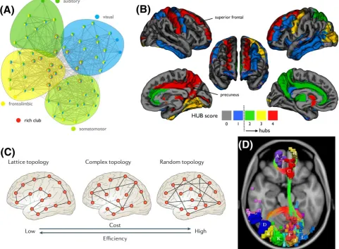
are often found universally across many species and imaging scales. Brain graphs aresmall‐worldnetworks that aremodularin structure.228Modular
small‐world networks are characterized by communities of nodes that are densely interconnected among themselves, predominantly with relatively
short connections, while also sparsely connected to other communities by a small number of long‐distance connections (Figure 6A). These densely
interconnected communities (modules) are hypothesized to facilitate network segregation and specialized information processing. The longer
con-nections interconnecting these modules facilitate network integration and distributed information processing. Modules in brain graphs tend to be
spatially localized and comprise cortical regions that perform specialized functions, such as visual, auditory or motor processing tasks.
Brain graphs also comprise a densely interconnected core ofhub nodesthat form arich club.229Hub nodes make connections with many other
nodes and serve as focal points for the divergence and convergence of neural information. Hubs are defined as nodes with large degrees, where the
degreeof a node is simply the total number of other nodes to which it is directly connected.230The nodes of brain graphs differ very substantially in
degree. Indeed, the distribution of nodal degrees in most brain graphs can be described by a truncated power law (scale‐free distribution), which
implies the existence of a small number of highly connected hub nodes. For a hub node to form part of the rich club, it must also be densely
con-nected with other rich‐club nodes. A rich club in general comprises nodes (hubs or non‐hubs) that are densely connected among themselves as well
as with other nodes. Non‐hub nodes of the club are called peripheral or local nodes. Rich clubs are synonymous with many kinds of natural and
engineered network. For example, major air transportation hubs are interconnected to an extent that is significantly greater than expected in
ran-dom networks with the same nodal degree distribution. While the hub nodes comprising a rich club are usually distributed across different modules,
they are also densely interconnected by long‐range connections. This suggests that the rich club is a network core that plays a crucial role in
inte-grating and coordinating the activities of specialized modules. Typical hub nodes comprising the rich club of brain graphs include the caudate,
thal-amus, precuneus, superior frontal gyrus and middle cingulate gyrus (Figure 6B).
Another property of brain graphs isnetwork economy.219Brain graphs are spatially embedded networks in which each node is associated with a
coordinate in Euclidean space and each edge has a physical length.135Long connections are considered costly to nervous systems in the sense that
they occupy more physical space and consume more metabolic resources.231A small number of long
‐distance connections is however crucial to ensure that information can be efficiently integrated between different modules. Spatially embedded networks that comprise only short
connec-tions are not very costly in terms of their energy and space requirements, but they are also not very efficient integrators of information. Indeed,
spatially embedded networks comprising only short connections are lattice‐like networks in which distant pairs of nodes must traverse many
con-nections to communicate. The number of concon-nections that need to be traversed, known as thepath length, can be drastically reduced with the
addi-tion of a small number of long‐distance connections.232Network economy refers to this trade‐off between the cost of a network's topology and
the efficiency with which that network can integrate information (Figure 6C). In practice, efficiency is quantified as the inverse of the path length
between all node pairs,233while cost is quantified as the sum of the physical length of all connections. Numerous studies indicate that nervous
systems have evolved to negotiate a compromise between network efficiency and network cost.234
4.3
|Comparing network properties between groups
Comparing the network properties of brain graphs between groups of individuals can reveal new insights into brain network organization in health
and disease (see Griffa et al10for an extensive review). Statistical inference can be performed on the connectome at many different scales. The
simplest data‐driven approach is to independently test the weights associated with each edge for a between‐group difference or a statistical
asso-ciation with some measure of cognitive performance. Network‐specific methods can be used to identify between‐group differences given the
net-work structure and correct for multiple comparisons. The netnet-work‐based statistic235,236is an example of one such non
‐parametric approach that identifies interconnected subnetworks for which the null hypothesis (of no differences between groups or no associations with chosen score) can
be rejected. Given that brain pathology seldom impacts a single connection in isolation,237these mass univariate approaches aim to identify
mul-tiple network elements that significantly differ in connectivity strength between groups. In many brain diseases, white matter connections provide
conduits that promote the spread and spatial propagation of a pathological mechanism,238,239and thus it is not surprising that disease
‐related con-nectivity effects often form interconnected subnetworks (Figure 6D).
Another approach to statistical inference is the testing of between‐group differences in global summary measures of network organization,
such as measures of network efficiency,219small‐worldness240and modularity.241Global testing is simple but lacks specificity, in that insight
can-not be gained into whether effects are distributed throughout the brain or confined to a specific set of nodes or edges. Finally, multivariate
statis-tical inference is growing in popularity and may play an important role in the future as datasets continue to increase in size and complexity.