The statistical analysis of point events associated with a fixed point

THE STATISTICAL ANALYSIS OF POINT EVENTS

ASSOCIATED WITH A FIXED POINT

Andrew B. Lawson

A Thesis Submitted for the Degree of PhD at the

University of St Andrews

1991

Full metadata for this item is available in Research@StAndrews:FullText

at:

http://research-repository.st-andrews.ac.uk/

Please use this identifier to cite or link to this item: http://hdl.handle.net/10023/7294

THE STATISTICAL ANALYSIS OF POINT

EVENTS ASSOCIATED WITH A FIXED POINT.

IMAGING SERVICES NORTH

Boston Spa, Wetherby

West Yorkshire, LS23 7BQ

www.bl.uk

TEXT CUT OFF IN THE

II

DECLARATION

a) I, Andrew B Lawson, hereby certify that this thesis has been composed by myself,

that it is a record of my own work, and that it has not been accepted in partial or

complete fulfilment of any other degree or professional qualification.

Signed Date

2

~

1\ \ )

q

/

b) I was admitted to the Faculty of Science of the University of St Andrews, under

Ordinance General No 12 on October 1986, and as a candidate for the degree of

Ph.D. on October 1987.

Signed Date "2-

7>

I \ \ \ '{

0

J

c) I hereby certify that the candidate has fulfilled the conditions of the Resolution and

Regulations appropriate to the Degree of Ph.D.

III

COPYRIGHT DECLARATION

A UNRESTRICfED

In submitting this thesis to the University of St Andrews I understand that I am

giving permission for it to be made available for use in accordance with the regulations of

the University Library for the time being in force, subject to any copyright vested in the

work not being affected thereby. I also understand that the title and abstract will be

published, and that a copy of the work may be made and supplied to any bona fide library

IV

ABSTRACT

This work concerns the analysis of point events which are distributed on a planar

region and are thought to be related to a fixed point. Data examples are considered from

Epidemiology, where morbidity events are thought to be related to a pollution source, and

Ecology and Geology where events associated with a central point are to be modelled.

We have developed a variety of Heterogeneous Poisson Process (HEPP) models

for the above examples. In particular, I have developed interaction and 8-dependence

models for angular-linear correlation, with their ML estimation and associated score/W aId

tests. In the Epidemiological case we have developed case-control models and tests.

The possibility of second-order effects being important has also led to the

development of Bayesian Spatial Prior (BSP) models.

In addition, we have developed a new deviance residual for HEPP models and

explored the use of GLIM for modelling purposes.

A variety of results were found in data analysis. In some cases HEPP models

provide adequate descriptions of the process. In others, BSP models yield better fits. In

general, the discrete case admits a simple spatial Poisson model for counts and does not

v

ACKNOWLEDGEMENTS

First, I should like to thank my main supervisor, Professor R M Cormack for

constant support and encouragement during the execution of this work. A number of lights

have been turned on during our many discussions and I am deeply indebted to him for such

illumination. I should also like to thank Dr P E Jupp who has acted as supervisor during

Professor Cormack's absence. As my research lies on the border between Spatial and

Directional data analysis, the combination of supervisors has provided a balance between

these areas.

Second, I should like to thank Jeremy Warnes for useful discussion concerning

Empirical Bayes methods and Kriging, and Dr T Rolf Turner (University of New

Brunswick) for use of his DELDIR program.

Third, I should like to thank Dr P Mason of the Institute of Terrestial Ecology,

Bush Estate for use of the Hebeloma Data Set, and General Register Office, Edinburgh for

Mortality and population data for Buckhaven - Methil and Bonnybridge. I should also like

to thank Dr Owen Lloyd and Dr Fiona Williams of the Environmental Epidemiology Unit,

University of Dundee, for access to the Armadale data set.

Fourth, I would like to acknowledge the excellent typographical work of Shiela

Wilson and Valerie Cobb, who have both provided speedy and accurate copy.

Finally, I should like to thank Pat for all her long-suffering patience and

TABLE OF CONTENTS

GLOSSARY

LIST OF FIGURES

LIST OF TABLES

LIST OF APPENDICES

INTRODUCTION

1 . Exploratoty Data Analysis

1.1 Kernel Density Estimation

1.2 Special methods

1.2.1 Kernel Interpolation

1.2.2 Covariate Extraction

VI

1.3 Preliminary Testing of Mapped Patterns

1.3.1 Radial Trend

1.3.2 Angular anisotropy

1.3.3 Radial-angular interaction

1.3.4 Example

2. Point Process Modellin" (Continuous)

2.1 HEPP model definition

2.2 Fixed-point HEPP models

2.2.1 The polar model and sampling window

2.2.2 Asymptotic Methods in Likelihood Analysis

2.2.3 Types of Intensity Model

2.2.3.1 The Radial component

2.2.3.2 The Angular component

2.2.3.3 Radial-Angular Interaction

2.2.4 Evaluation of the Normalising Constant (A(A»

2.3 Likelihood Methods for HEPP models

2.3.1 Single factor intensity models

2.3.2.1 ML estimation

2.3.2.2 Hypothesis tests

3. Continuous Model: Extensions

3.1 Observed Heterogeneity

3.1.1 Case - Control Score Tests

3.1.1.1 Case a) Radial Trend

VII

3.1.1.2 Case b) Angular Concentration

3.1.1.3 Case c) Peaked-Radial Effect

3.1.1.4 Case d) Interaction Effect

3.2 Unobserved Heterogeneity

3.2.1 Harmonic Intensity Terms

3.2.2 Spatial Prior Structure for Intensities

3.2.2.1 Cox Process Model

3.2.2.2 A Bayesian Spatial Prior (BSP) Model

4. Continuous Model: Goodness-of-Fit of Residual Analysis

4.1 Global Goodness-of-Fit

4.2 Residual Analysis

4.2.1 Binned Residuals

4.2.2 Individual Residuals

4.2.2.1 Deviance Residuals

4.2.2.2 Examples

4.2.2.3 Autocorrelation and Deviance Residuals

4.2.2.4 BSP Individual Residuals

5. Discrete Model: Introduction

5.1 The Human Morbidity Pattern

5.1.1 Functional forms for E ~

5.1.2 Likelihood Methods

5.1.2.1 Maximum Likelihood Estimation

5.1.2.1.2 Angular Concentration

5.1.2.1.3 Radial-Angular Interaction

5.1.2.2 Hypothesis Testing

5.1.2.2.1 Exponential Trend

5.1.2.2.2 Angular Concentration

5.1.2.2.3 Radial-Angular Interaction

5.1.2.3 General Testing with Observed Heterogeneity

5.1.2.4 Unobserved Heterogeneity

5.1.2.4.1 Harmonic Hazard Tenus

5.1.2.4.2 Spatial prior structure for hazards

5.1.3 Discrete Model: Goodness-of-Fit and Residual Analysis

5.1.3.1 Global Goodness-of-Fit (OOF)

5.1.3.2 Residual Analysis

6. Variants of the Continuous/Discrete Models and Hazards

7.

6.1 Model Variants

6.2 Hazard Variants

HEPP Models on OLIM

7.1 Normalising Constant Models

7.2 Numerical Approximation

7.3 Probabilistic Approximation

7.4 Integral Approximation Accuracy

7.5 One Dimensional Models

7.5.1 The von Mises Distribution

7.5.1.1 Numerical Comparison

7.5.2 A Test for 'von Misesness'

7.5.3 The Fisher Distribution

7.5.3.1 Data Example

7.5.4 Spatial HEPP Model

8.1 Mooel Simulation

8.1.1 Continuous Models

8.1.1.1 HEPP Models

IX

8.1.1.2 Bayesian Spatial Prior Mooels

8.1.2 Discrete Models

8.1.2.1 Multinomial Models

8.1.2.2 Bayesian Spatial Prior Models

8.2 Test Statistic Behaviour

8.2.1 Sampling Distributions

8.2.2 Numerical Power Studies

8.2.2.1 Continuous data sets

8.2.2.2 Discrete data sets

9. Analysis of Data Sets

9.1 Data Sets A, Band C

9.1.1 Respiratory Cancer Deaths (Data Set A)

9.1.2 Bronchitis and Pneumonia Deaths (Data Sets B, C)

9.1.1.2 Bonnybridge (Data Set B)

9.1.2.2 Buckhaven-Methil (Data Set C)

9.2 Data Sets D, E, F

9.2.1 Hebeloma Sporophores (Data Set D)

9.2.2 Oak Bark Beetles (Data Set E)

9.2.3 Lupinus Arboreas (Data Set F)

9.2.4 Volcanic Ejecta (Data Set G)

9.2.4.1 The 1935 example

9.2.4.2 The 1937 example

9.2.4.3 The 1938 example

DISCUSSION and CONCLUSIONS

REFERENCES

x

Glossary

Listed below are the standard set of symbols used in this thesis. Any variation in

this notation is defined where it is required.

N(A)

regIon

A

!AI

E(X)

R,<l>

number of events in a region A.

a suitably defined area of the plane.

region label.

Lebesgue measure of A in R2 (area)

Area of i-th Dirichlet tile.

expectation of a random variable X.

random variables describing the radial and angular behaviour of points.

Usually 0

<

<

0< <l> < 2n.

ro radius of circular sampling window.

r,cp realised values of random variables Rand <l>

r

x,y cartesian coordinates of point location

~ cartesian coordinate pair (x,y)

br(t) disc with centre

r

R the real line

p

A(A)

~n

gU:)

p

n~

E~

rij

Zn/Fn

XI

the surface of a 1-d sphere (the circle)

the intensity function at r

constant baseline intensity

J

A

A(.) evaluated at point i

n

I

i=l

(n xl) vector of mean surface values

(n x 1) vector of linear predictors

linear predictor at r

number of events in region .t

number of regions

hazard of any event in region .t

hazard associated with individual i in region .t

total population of region .t

expected number of events in region .t

population of i-th age, j-th sex group in region .t

national event rate for i-th age and j-th sex group

number of age groups

XII

0-

!X (Pa xl) vector of parameters

Pa,Pb number of parameters

Kn (n x n) covariance matrix

d(i,j) euclidean distance between points i, j

0 2 variance of a Gaussian Process

Ra covariance range parameter

XIII

List of Fieures

1) Data example maps:

a) Data set (A) : Annadale

b) Data set (B) : Bonnybridge

c) Date set (C) : Buckhaven-Methil

d) Data set (D) : Hebeloma sporophores 1975, 1978

e) Data set (E) : Oak: Bark Beetles

f) Data set (F) : Lupinus arboreas

g) Data set (G) : volcanic ejecta 1935, 1937, 1938

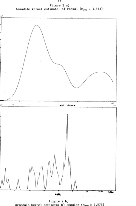
Figures 2 to 8 consist of Gaussian kernel estimates of the a) radial, b) angular

marginal distributions for the above data sets. Display c) is the surface 2-dimensional

kernel estimate for the data set. All estimates were obtained using likelihood

cross-validation. Figures 2) to 5) are point estimates and figures 5) to 8) are count estimates.

2) Armadale (A)

3) Hebeloma (D)

4) Lupinas (F)

5)

6)

8) Oak Bark Beetle (E)

9) Covariate extraction

a) Annadale case-control i) popUlation, ii) heart disease case control, iii)

cancer, iv) extraction

b) Bronchitis and pneumonia deaths with expected deaths extracted :

Bonnybridge

c) Bronchitis and pneumonia deaths with expected deaths extracted:

Buckhaven-Methil

10) Simulations: M(1l0, lC+'I'r)

11) Simulations: a-dependence,

12) Marginal g(<I» of interaction M(IlO, lC+'I'r)

13) i) Point maps of deviance residual test data sets

ii) Probability plots: CRICK, REDWOOD, PPSDRES, PPCNRES,

Annadale marginal angular density (a-e)

14) Annular-sector method for regional integration

15) Point map: HEPP simulation on unit square (n = 30 points)

16) Simulations of a) Hebeloma 1975 data

b) volcanic ejecta 1935 data

17) BSP simulation a) covariance range

(a)

b) variance (cr2) variation

c) trend with range (a) variation

xv

19) Discrete simulation: a) angular concentration

b) angular interaction

c) concentration and interaction

20) Discrete BSP simulation: a)

a

b) a = 0.1, (32 = 2

21) Discrete BSP simulation: a) a = 1, (32 = 5

b) a = 1, (32 = 0.5

c) a = 10, (32 = 1

d)

a

22) continuous power studies: asymptotic critical regions

23) continuous power studies: monte carlo critical regions

24) discrete power studies: asymptotic results

25) discrete power studies : distance test comparison

26) Annadale: a) point map

i) respiratory cancer

ii) heart disease

b) respiratory cancer expected death swface

27) Deviance Residual displays: Annadale

a) fitted values, b) radial distance, c) angle, d) normal plot, e) surface view,

t) surface contour map

a) enumeration distinct map (with inset location map)

b) SMR and death count surface (Bronchitis and Pneumonia)

29) Anscombe Residual displays: Bonnybridge

a) fitted values, b) radial, c) angle, d) normal plot,

e) surface view, f) surface contour

30) Buckhaven-Methil:

a) enumeration district map

b) SMR and death count surface (Bronchitis and Pneumonia)

31) Anscombe Residual displays: Buckhaven-Methil : reduced data set:

a) surface view, b) surface contour, c) fitted values, d) normal plot

33) Deviance residual displays: Hebeloma 1975

a) fitted values, b) radial distance, c) angle d) normal plot,

e) surface view, f) surface contour

34) Deviance residual displays: Hebeloma 1978

a) fitted values, b) radial distance, c) angle, d) normal plot,

e) surface view, f) surface contour

35) Standardised residual displays: BSP model fit: Hebeloma 1975, 1978

a) fitted values, b) normal plot, c) surface view, d) contour map

36) Oak log locations : Oak Bark Beetle data

37) Count map: Oak Bark Beetles

XVII

a) -f) as for fig (27)

39) Deviance residual displays: Lupinus Data

a) -f) as for fig (27)

40) Standardised residual displays: BSP model: Lupinus data

a) fitted value, b) nonnal plot, c) surface view

d) surface contour

41) Deviance residual displays: 1935 volcanic bomb data

a) -f) as for fig (27)

42) Standardised residual displays: BSP model: 1935 volcanic bomb data

a) -f) as for fig (35)

43) Deviance residual displays: 1937 volcanic bomb data

a) -f) as for figure (27)

44) Standardised residual displays: BSP model: 1937 volcanic bomb data

a) - d) as for fig (35)

45) Deviance residual displays: 1938 volcanic bomb data

a) -f) as for fig (27)

46) Standardised residual displays: BSP model: 1938 volcanic bomb data

a) - d) as for fig (35)

List of Tables

1) Preliminary tests: data set A

2) Optimisation of M(~, 1(+'JIr) models on NAG (Appendix XII)

3) Numerical accuracy results I-D weights

4) Numerical accuracy results 2-D weights

5) GLIM model results for the VOL 35 data example

6) ML results for Armadale (Data Set A)

7) Armadale: a) case-control and other model results

b) kernel score tests

8) GLIM model fits for Total Deaths: Bonnybridge

9) Score Test results: Bonnybridge

10) ML estimates of 1(, 'JI, ~ : Bonnybridge

11) Glim model fits for total Deaths: Buckhaven-Methil

12) Score test results: Buckhaven-Methil

13) ML estimates for 1(, 'JI, J.lO : Buckhaven-Methil

14) Summary of Models for Bonnybridge and Buckhaven-Methil

15) Glim model fits for 1975, 1978 Hebeloma examples

16) Exploratory tests for Hebeloma Data

17) Glim model fits for Beetle Data: Polar Model

XIX

19) GLIM model results for Lupinus data

20) Exploratory tests for Lupinus data

xx

List of Appendices

I Computational Methods

II Simulation Methods

III Research Papers

N Score Tests for Peakedness

V Moments and other elements of the characterisation of the Interaction von Mises

Distribution (M(J!O, K+\jff))

VI Derivation of Score and Wald Tests for Continuous and Discrete Models

VII GLIM macros

VIII Parameter and variance-covariance matrix approximations using the Delta Method

IX Observed Information Matrix for the Case-Control Score Test for interaction

X Asymptotic Sampling Distributions for test statistics

XI Data sets

XXI

Introduction

The purpose of this reported research is the development of statistical

techniques for the analysis of a point process associated with a fixed point. The

motivation for this work lies in its application to the analysis of problems in

Environmental Epidemiology and Ecology and Geology.

The detection of association between deaths recorded within an area and a

pollution point source, (e.g. a factory chimney) is an example of such a problem found

in environmental epidemiology. Published examples of such data are given in Lloyd

(1982) and Lenihan (1985) and Carstairs and Low (1986).

In addition, there are a number of examples of data sets in Ecology where the

spatial distribution of events is related to a fIxed central point. Last et al (1984), Ford et

al (1980) and Mason et al (1982) give examples of the spatial association of fruitbodies

of sheathing mycorrhizal fungi around birch trees (Betula pendula). Yates (1983) has

cited an example of the radial dispersion of oak bark beetle (Scolytus intricatus). The

dispersal of seeds from a single plant would represent another example of such

association. Palaniappan et al(1979) give an example of colonisation of a waste tip site

by Lupinus Arboreus. The distribution of volcanic bombs/tephra after a volcanic

eruption is an example of a geological event which involves dispersal by air. Minikami

(1942) gives examples of a series of such events. Figure 1 displays examples of each

data set.

Association with a single fIxed point can be considered to be a special case of

association with a realisation of another stochastic process of objects. Berman (1986)

gives an example of modelling association between a point process (mineralisation

sites) and a line process (faults) in a geological application. Conditional on the

case of a single fixed point is a specialisation of Bennan's problem. Stoyan et al

(1987) give other examples and some descriptive measures of association. The study

of association between cancer cases and electromagnetic fields is a medical example.

The examples from Epidemiology and Ecology and Geology above, may show

similar data structures but differ in that the hypotheses of interest are different and the

level of data aggregation may vary considerably. In the epidemiology example, we are

concerned with evidence for association between the fixed point and events to assess

ultimately whether there is a causative link between these items. Hence, we are

concerned with 'detection' of the imprint of a pollution source on a population of,

possibly, variable susceptibility.

In the Ecological and Geological examples we are concerned with a movement

out from a centre, either through dispersal in air or growth underground. In these

examples, detection of the centre of dispersal is not important. However, appropriate

modelling of this dispersal is important.

Different levels of data aggregration tend to lead to differences between the

modelling approaches required by these two types of example. In the epidemiological

example, a realisation of death locations may only be available as counts within census

enumeration districts (eds), and hence arbitrary regionalisation of a point process must

XXIII

Data Examples

The data sets considered in this work are as follows:

Epidemiological examples

A) Addresses of respiratory cancer death certificates for Armadale, West

Lothian. The number of addresses (n) is 49. For this example the population structure

of the area is available from 18 census eds. Deaths have been recorded for the period

1968-1974, and the 1971 census has been used as a population base. This data set was

first analysed by Lloyd (1982) as part of a study of the perceived environmental hazard

from a steel-making complex in central Armadale.

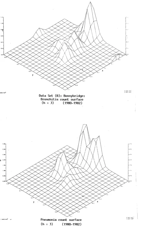
B) Counts of Bronchitis and Pneumonia deaths (1980-1982) in eds within a

5km radius circle of a chemical reprocessing plant (OR 835815); Denny-Bonnybridge

area, Central Scotland. The number of eds studied is 200. Population information is

available from the 1981 census.

This data set relates to the analysis made by the Lenihan Committee (Lenihan

(1985)) on a perceived environmental hazard thought to relate to the Rechem Chemical

reprocessing plant.

C) Counts of Bronchitis and Pneumonia deaths (1980-1982) in eds within a

3km radius circle of an industrial complex (OR 366004); Buckhaven-Methil area,

Eastern Fife. The number of eds studied is 62. Population and deprivation information

are available from the 1981 census.

This data set is from an industrial area with a central industrial complex

surrounded by domestic housing areas. No environmental hazard has been postulated

The above data sets represent a spectrum of data aggregation level, from set A)

which consists of exact locations and regional covariates to set B) where death counts

in eds are available with population totals. Set C) can be regarded as a control data set

and will be used in informal comparisons at a later stage.

Ecological Examples

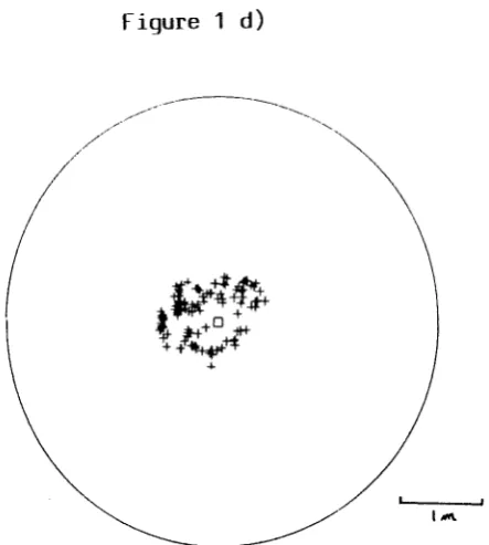
D) Locations of Hebeloma Sporophores around a birch tree (1975, 1978)

within a 5m square window. The number of point locations is 115 and 41 respectively.

No covariate information is available.

This data set was analysed by Last et al (1984) and similar data sets were

modelled by Byth (1980).

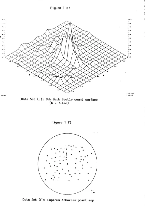
E) Counts of radio-labelled oak bark beetles found on experimental logs set at

predetermined points around a central release point within a radius of 76m. The

number of marked beetles is 115, the number of unmarked beetles is 366.

This data set was analysed by Yates (1983) and contains total populations at

each location.

F) Locations of Lupinus arboreus plants found over a 6 year period around a

central source plant on a waste tip site. The number of plants is 76.

This data set was analysed by Palaniappan et al (1979). No covariate

information available for this example.

The above ecological data sets represent dispersal from a central point and

consist of exact point locations

«D)

xxv

Geological Examples

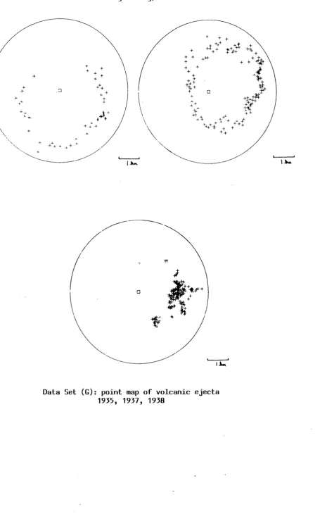
G) The locations of volcanic bombs after eruptions of Mt. Asama, Japan

(1935, 1937, 1938). These data sets consist of mapped bomb locations found after the

eruptions of Apri120th 1935, April 10th 1937 and June 7th 1938. These data were

presented by Minakami (1942). This data is characterised by dispersal under prevailing

wind, and shows a simpler pattern than the biological examples considered above. No

covariate information is available. Figure 1 a-g displays the data sets. In the case of

count data a surface representation is given.

Spatial Models

The data examples given above have some common features. First, the basic

unit of data is a point location or a count of points in a region. Second, the

observations are measured relative to a fixed point. Third, the spatial pattern which is

to be described is characterised by slowly varying point intensities i.e. we are

concerned with first-order spatial properties or spatial trend.

Observations in the form of point locations or counts suggest a Point Process

model could be appropriate. Location relative to a fixed point suggests that the Point

Process should be modelled in polar coordinates (r,cjl).

Finally, first-order properties can be modelled by an intensity function

dependent on location, i.e. A(X), and it is natural to consider a heterogeneous Poisson

Process (HEPP) as a basic model. An HEPP model may be thought appropriate for

fixed-centre data sets as the r and q, components can be related to the central point and

relatively simple parametric forms for the (r,q,) distribution can be specified.

Essentially, a bivariate distribution underlies this model assumption.

Second-order properties of point processes, i.e. their covariance structure, are

XXVI

concerning the modelling of such patterns (see, for example, Diggle (1983); Ripley

(1981, p 155-168; Ripley (1988, p 49-67)). In the examples considered here, we do

not consider second-order effects, except where underlying environmental

heterogeneity will be modelled with a spatial prior density. This approach can be

justified by the fact that we consider the spatial distribution of diseases with no known

clustering aetiology (Bronchitis, Pneumonia, Respiratory Cancer), and of dispersal of

plants, insects and volcanic ejecta from a central point. In either case, first-order effects

must be modelled even though some environmental or subject heterogeneity may

produce apparent clustering.

A number of methods are available for incorporation of such prior spatial

structure, and we will review these alternatives in the following chapters.

First of all, we consider two basic types of model which could be applied to the

above cases. In chapter 2 we outline a continuous model which could be applied in

most data examples. Chapter 5 deals with a discrete model for human population

structure which is related to the proportional hazards model in the time domain. This

model was developed to allow the incorporation of covariates defined on individual

susceptibles in the population considered.

The two basic models represent different ends of a spectrum from a

homogeneous environment (continuous model) to a discretisedlheterogeneous

environment (discrete model). However, each model can be modified to move closer to

the other formulation, and such modifications will be discussed in the following

1

CHAPIER 1

1 . Exploratory Data Analysis

Exploratory methods for mapped point process data have developed traditionally via

visual inspection of point maps to description of the intensity surface of the process by

density estimation (see, for example, Byth (1980), Diggle (1981)). In most data examples,

a stationary process is to be described and the isotropy of this process has led to the

development of toroid ally-corrected density estimates as a basic tool in graphical

exploration. Alternative graphical techniques which depend on functions of point locations

can also be utilised, and there appears to be scope for the application of multivariate EDA

methods in this area.

Information about general spatial structure can be obtained from the Dirichlet

tesselation or Delaunay triangulation ofthe points (see, e.g. Sibson (1980)). As the area of

a Dirichlet tile (A) is related to the local point density, then 1/A is an intuitively appealing

local intensity estimate. Hence a Dirichlet tile map yields an intensity 'picture'. The

Delaunay triangulation yields a similar pictorial effect but also demonstrates the convex hull

shape of the process. Convex hull peeling (Green, 1981) also yields information about

anisotropic structure and shape.

The data examples considered here are not stationary and show anisotropy. In

addition, as these examples are related to a fixed point, it is possible to consider the

marginal structure of the radial and angular components of the processes.

Although the above general EDA methods are applicable in these examples, some

adaptations of existing methods and new methods have been derived to account for these

Figure 1 a)

+ + +

+

+ + +

+ ₊ +

+ .;-+

+ + ₊₊

0 ++

.;!t+ ++

-I't + #.p-+ + +-t+ + + + +

+

I " "

Data Set (A): Armadale:

Z O.G

0.'

1.~

Z ,.OO

>.00 0."

3

Figure 1 b)

Data Set (B): Bonnybridge: Bronchitis count surface

(h = 3) (1980-1982)

Pneumonia count surface

(h = 3) (1980-1982)

f"

r' ,

r" "

I

r

L"

l:,

f

0.'

lAll< wle;

... ~, I~ .1 G ~

r'"

r'~'

r"'"

I

f"

f '

1'0.,,\:;

0,'

2 ~'I('~ -.10

z

z

Figure 1 c)

Data Set (C): Buckhaven Methil: Bronchitis count surface

(h

=

Pneumonia count surface

5

Figure 1 d)

,""-Data Set (D): Hebeloma Sporophores point map 1975, 1978

+++ _~

t

*

+ ₊

~ :t +

*

+ ₊₊ 0

++

+ +

++

"1

"1

• -'1

"1

zJ

figure 1 e)

Data Set (E): Oak Bark Beetle count surface

(h

=

figure 1 f)

+ + + + + + + + + + + ++ _{+ +}

+ + + +

+ ₊

+

++

+ _{+ ++ +}

+ ₊

+ _{+ ++}

+ +

+ _{+ +}

+ >to _tB +

+ + + +

+ + +

+ + _{+ +}

+ + + + + + +

+ +

+ + +

+ ++ + ₊ +

Data Set (f): Lupinus Arboreas point map

10.0

5.'

...

I.' I.'

...

..

Z AXIS .IO~·

\\"

+

+ +

+

+

7

Figure 1 g)

+

+ +

+

+++

+

\

+ :t

++\-'-

\

_\

+

\

'",- 4 . . l

-"~"'~/

+ + +

++t-+

+ +

+ + +1 +{+

+ o

1. 1 Kernel Density Estimation

Diggle (1981 ,p 55) has proposed a general toroidal edge-corrected kernel method

for spatial point maps. The estimates thus produced can be viewed as contour plots or

isometric views. Usually contours hold more detailed information, but isometric views are

useful for general assessment

When point data shows marked non-stationarity on visual inspection then it is

inappropriate to use toroidal edge-correction in density estimation. The only method which

accounts for edge effects is to use a guard area and, by implication, view a percentage of

the map area at each edge as a border. Hence, standard two-dimensional kernel estimates

can be used.

As the nature of the kernel is not critical, (compared to the choice of smoothing

parameter), we have used a two-dimensional Gaussian kernel due to its computational

simplicity. The choice of smoothing parameter (h) is however, important, as arbitrary

over-smoothing can occur. Epanechnikov (1969) gives an IMSE criterion for obtaining an

optimal h value which can be evaluated for specific target distributions. However, as we

do not wish to make specific distributional assumptions, we have used likelihood

cross-validation to estimate h opt. It is important to note that quite marked differences in h opt

can be produced by these two criteria. Hence, as cross-validation is less parametric it is

preferred.

The marginal radial or angular density of points can also be estimated. This form of

density estimation is one-dimensional, but has to be adapted to the truncated positive real

line for radial estimation, and to the circle for angular estimation. The first case may

require reflection of data about the origin (Boneva et aI, 1971). In addition, at the

IMAGING SERVICES NORTH

Boston Spa, Wetherby

West Yorkshire, LS23 7BQ

www.bl,uk

PAGE MISSING IN

where K(.) is a kernel function

h is the smoothing parameter

C is a normalising constant

n is the number of points.

We can introduce a new variable Z(Xi), say measured at Xj, and re-write (1.1) as

1 n

2(x)

=

L

i=l

(1.2)

Here K(.) acts as a smoothing operator on z, and hence this operation can be used

to interpolate Z to new locations. One advantage of this method is that it ensures that if Z is

restricted to the positive real line then 2(x) will be non-negative. This is not true of

methods such as Universal Kriging, although log normal Kriging would protect against

this effect. Hence, interpolation of counts can be directly achieved without the requirement

of transformation.

The above method has been little documented (see, e.g. Ramlau Hansen (1983),

Titterington (1985)) and the author knows of only one published application of this method

where standardised mortality ratios (SMRS) are interpolated in time (Breslow and Day,

1987, pp 193-197). We have applied this method in the two-dimensional case to count

data in regions. An example of this is the interpolation of region populations to the loci of a

point process. This method also allows the exploratory examination of count data by

contouring of an interpolated mesh. This method has been used for preliminary analysis of

"

I

11 Figure 2 a)

Armadale kernel estimate: a) radial (h cv

=

J

~

\

Figure 2 b)

Armadale kernel estimate: b) angular (h cv

=

z

Figure 2 c)

0)

J

b)

~r

i

,~

oj

I

i 1

I

J

I

13

Figure 3 a), b)

Hebeloma kernel estimate: a) radial 75:h

=

b) angular 75:h

=

l

Figure 3 a), b)

Hebeloma kernel estimate: b) radial 78:h = 0.0427 b) angular 78: h

=

l~~

"~I

I

I

'I

I~

I I

1

I

\ II

II

radial distance

15

Figure 3 c)

Hebeloma kernel estimate: c) surface view 75:h = 0.0497; 78:h = 0.123

i

1

,~ I

1

"1

I

z

r

"1

r'

r

"1

I

1 r

Figure 4

Lupinus Arboreas kernel estimate: a) radial (h

=

I

radial distance

angle

Figure 4

Lupinus Arboreas kernel estimate: b) angular (h

=

y

17

o

~~~',.~~~~~~~--~.,--~~~

. . . J

, MII._.'

figure 4

X ~\U''''I ... - l

Figure 5

Volcanic ejecta kernel estimate: 1935 a) radial (h

=

/

!

/

/

/ '

radial distance

'ngl,

Figure 5

Volcanic ejecta kernel estimate: 1935 b) angular (h

=

\

\

..

19

,

~

y'j-J

I

I

I

Figure 5

Volcanic ejecta kernel estimate: 1937 a) radial (h

=

/

'---~~~---r---r---<---'---"---or---,-,.,~

radial di~tance

,ij

"

angle

Figure 5

y •.•

-0.1

Figure 5

Volcanic ejecta kernel estimate: 1937 c) surface view (h

=

'.0

'.0

Figure 5

Volcanic ejecta kernel estimate: 1938 a) radial (h

=

.,

angle

Figure 5

23

y •

,.

I;i

@

ilr

'lrl

;.

.

.... r'.,G _{"n.,ol ~_"'ICW!."~}

X

figure 5

. /

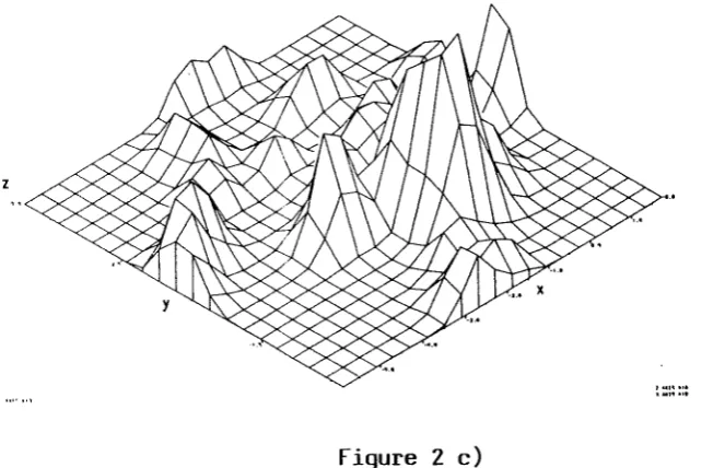
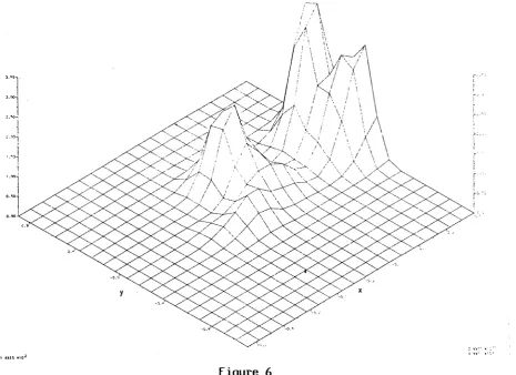
Figure 6

Bonnybridge kernel estimate: Bronchitis: a) radial (h

= 3.07)

/

radial dl~tan(e

:~---~---=---~,'---~,~'---~E---~'-·----~"---~"

angle

Figure 6

Bonnybridge kernel estimate: Bronchitis: b) angular (h

=

25 Figure 6

Bonnybridge kernel estimate: Pneumonia: a) radial (h = 3.07)

/

/

1/

/

/

/ r

-\

\ \

\

\,

I

---.---~-.---~---" "

Figure 6

radial di5tance

" ?

angle

Figure 6

Bonnybridge kernel estimate: Bronchitis: c) surface view (h =

'~l

"~l

"~1

z ; .. )');

,<,~

y

, . I r' .

7.773)'

, .. ", i

.. "

Figure 6

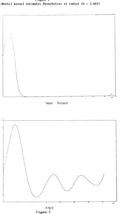
27 Figure 7

Buckhaven-Methil kernel estimate: Bronchitis: a) radial (h = 3.483)

\

\

radial distance

~'f---~---'

I

/\

! \

\

_\

\

\

\

\

r

I

I

,I

I

i

I

i

\

\

\

(\\

~/

---~---~ ~ij

angle

Figure 7

Buckhaven-Methil kernel estimate: Bronchitis:

l3 ... I,

XIO'

Figure 7

Buckhaven-Methil kernel estimate: Pneumonia: a) radial (h

=

,

-\ \ \

I

\ \

I

\

radial distance

'/-'

-( "

. \

.I \

\

!

-"

a no I e

Figure

29

Figure 7

f "

.,

I .. n •• ,

.... <."

Buckhaven-Methil kernel estimate; Bronchitis: c) surface view (h

=

z

, ... " ...

.... n ...

"l~~

---"I

---1

I i

'\

I

,I

I

,

'.

\ I

0

,

~

,

.

,

;\

;\

n

A

, 20 _'" .0

radial di~tance

Figure B

Oak Bark Beetle kernel estimate: a) radial (h

=

'1'1"

" , . _ - - - ,

" I

I~

l

"f

I

/

,J---.---,---t.---",--.--,.---,.----~---{

anqle

Figure B

31

.,

1 _,

'l

1

o

~ .• 't-. -."-,,-••• ---:'C;---""'-T,---=--~--""""'----~J.;---t

'Ult." X not'ca.-,.IPtI.,.-S

Figure 8

Oak Bark Beetle kernel estimate: c) surface view (h

=

r

c·

r'

r , r

r

t

r

,

1.2.2 Covariate ExtractioD

The above methods are usually sufficient to describe the spatial structure of points

or region counts in a mapped area. However, spatially-distributed covariate information is

often associated with such data sets, and it can be important to examine the effect of such

information on the spatial point process.

For example, the location of deaths in an area is related to area population, in that

higher densities of populations should show higher numbers of deaths. This is often

accounted for in regional count data by comparing a regional count to the expected number

in the region based on its population structure (SMRS).

We have developed a new method, based on kernel estimation, for the extraction of

baseline/covariate information.

Defme the point process to be governed by an intensity

A *(x)

=

where H(x) is a baselinelcovariate process and A(X) is an underlying spatial intensity. H(x)

could be a population process or even a case-control point process (see Diggle (1989».

We now introduce a kernel estimator of the intensity

(1.4)

where

1\

HQij) is the estimated covariate process evaluted at lU.

1\

Note that H(Xi) can be an intensity estimate of a case-control point process or the

interpolation of a real valued covariate to Xi.

~W

case-33

figure 9 a)

Armadale case control i) population surface (h

=

y

x

'unn,'

f'''

r "

F:

t·,.

~ ...

f"

f'"

''''S .. t '

• "n·"

Armadale case control ii) heart disease surface (h

=

z

:::::::'

c

Armadale _case Figure 9 ) _a

35

Figure 9 b)

(Bronchitis)

Bronchitis and Pneumonia deaths

with expected deaths extracted: Bonnybridge (h

=

z

...

Figure 9 c)

",

:j

z,

z

y

Bronchitis and Pneumonia deaths

with expected deaths extracted: Buckhaven-Methil (h

=

Bronchitis

Pneumonia

.. Population

'''I''''

37

control example, is based on the fact that any value> 1 is in excess of the basline

case-control. A similar interpretation is possible for other covariates if they are suitably

normalised over the window area. Figure 9a) display the results of such extraction for data

set A with a case-control point process of cardio-vascular disease. Figures 9 b), c) display

the results of such extraction for data set Band C for Bronchitis deaths and baseline

process of expected number of deaths.

1.3 Preliminary testing of Mapped Patterns

Visual inspection of point maps and contoured intensity surfaces demonstrate the

general structure of data sets. In our examples, the dominant structure appears to be

non-stationarity with marked anisotropy around the central point. There is only limited evidence

of clustering.

As our aim is to assess whether there is evidence of spatial trend around the central

point, we can employ simple statistical tests to assess trend components prior to statistical

modelling.

1.3. 1 Radial trend

Association with a central point may be displayed by a gradient or trend over radial

distance from the centre. A number of tests are available for testing the null hypothesis of

uniformity against trend alternatives for a 'radial-only' effect. Cox and Lewis (1966)

derived the uniformity test, which in our case is given by

n

IIi -

~ro

U

=

ro

~ l~n

where ri

=

ro

=

n

=

Cliff and Ord (1981, p 107) also suggest a spacings test which can be adapted to annular

areas i.e.

n

S

=

L

.i=I

where A(j)

=

(1.6)

Under the assumption of complete spatial randomness (CSR), we have E(S)

=

(n-1)/2 and var(S)

=

positive values imply regular spacing and negative values imply clustering or

non-stationarity. The test given in (1.5) is the score statistic derived from the assumption of a

heterogeneous poisson process with exponential trend i.e. A.(r)

=

for any monotone alternatives (Gart and Tarone (1983». Both U and S have an asymptotic

standard normal distribution.

As the radial effect could be peaked as opposed to monotone decreasing we may

also test for a Weibull shape parameter:

Ho:

=

statistic. The detailed derivation of this test is given in Appendix IV. This derivation is

given as this author is unaware of such a test for a truncated Weibull in the literature.

In the case of count data it is also possible to apply a uniformity test like (1.5) by

assuming that the hazard in each region (~) is E~

=

39

(1.7)

p

where

L

.(=1

(n T

=

f

n~

~,

~-th

xi

derivation of this test is similar to that given in Breslow et al (1983).

1.3.2 An2uJar Anisotropy

If angular uniformity is to be tested, then a variety of tests are available and are well

documented (e.g. Mardia, 1972). Watson's U2 test, Rao's spacing test or the Rayleigh test

are well known examples which can be employed to detect deviations from angular

uniformity.

For the case of counts in regions it is possible to use a new test for angular trend:

[

~

cos (ckllo)[nt - NeEtl

r

Th=---~---~---N{

~

Et

cos2(~k-~)

-

(~Et cos(~t-llo)

H

~

Et)]

p

where Ne

=

nTIL

.(

and ~ = tan-1(NS/NC) and

p

NS =

L

.(

p

NC =

L

.(

where </>.( is the angle of the R-th region measured from the central point. Th has an

asymptotic

xi

1.3.3 Radjal-aneuJar interaction

Separate tests of radial or angular uniformity ignore the possible effects of

interaction or correlation between radial and angular components and hence could be

misleading if carried out in isolation. A number of tests are available which measure

general angular-linear correlation (e.g. Jupp and Mardia, 1980). However, for the case of

a radial-angular interaction a new test has been developed by the author.

n n

L

L

R

VVs=~---~---- (1.9)

where

n n

S =

L

L

A(K)

=

and A'(K)

=

where 11 (.) and 10(.) are modified Bessel functions of the first kind of 1st and Oth order

41

The detailed derivation of this test is given in Chapter 2.

For counts in regions a similar score statistic (eq 77) has been derived. Details of

this test are given in Chapter 5.

1.3.4 Example

We now consider where the above preliminary testing can be employed prior to

modelling of spatial pattern. (We consider all data sets more fully in Chapter 9) Data set A

consists of death certificate addresses, and their spatial distribution may be related to the

underlying population structure or to a case-control point process. In this example, we

have utilised the 1971 census total population counts for 18 eds in the Armadale area, as a

population covariate. In addition, we have selected cardio-vascular disease mortality as a

disease which closely matches the age-specific-aetiology of respiratory cancer but should

be little affected by an air pollution source (Lloyd, 1982). Hence, we utilised death

certificate addresses for this disease as a case control point process.

Figures 9a show the effect of using likelihood cross-validated kernel estimates for

population, case control, and respiratory cancer separately.

We have also employed 'covariate extraction' to this data set by extracting the

case-control density estimate from the data. The result is given in Figure 9a). The individual

density surfaces show a marked concentration of respiratory cancer to the south west of the

foundry area, while the population structure and case-control show higher concentrations in

the northern areas. The extraction of the case control produces a single 'dramatic' peak of

respiratory cancer in the north west sector. This is not at all apparent from inspection of the

individual surfaces. Lloyd (1982) has shown that the results of wind tunnel experiments,

north-westerly direction from the foundry. Table 1 displays the results of applying the

preliminary tests listed above to the Armadale data set.

Table 1 Preliminary Tests: Data Set A.

The results of preliminary statistical tests for spatial trend effects in data set A, with

n

=

L : radial uniformity test (1.5)

S : spacings test (1.6)

W : Weibull Shape test

R : Rayleigh test

U2 : Watson's U2 test

Ws: Interaction score test (1.9)

M : Mardia rank correlation test.

All tests have an asymptotic standard normal distribution except M which is -

X~,

and

U2

tests for each statistic, as the asymptotic distributions quoted above may not hold in this

example.

L S W R U2 _{Ws M}

-4.231 * -3.394* 5.412* 0.544* 0.814* 2.39* 7.48*

43

The radial tests (L,S) both show significant non-unifonnity and the negative sign

suggests possible clustering or non-stationarity The peakedness test (W) also shows a

significant result with the radial parameter estimated under the null hypothesis. This

suggests that a peaked effect occurs in the data. Watson's U2 test shows high significance

which suggests that preferred orientations exist in the data. Both the interaction score test

(Ws) and the rank correlation coefficient are significant and this also suggests a significant

correlation exists between radial and angular components. Hence, preliminary tests

confmn the visual evidence that there is a preferred direction and strong radial trend in the

original data. The case-control extraction, however, suggests a similar result although the

direction of the effect is different from that suggested on visual inspection. A similar

CHAPTER 2

2. Point Process Modellin2 (Continuous)

We assume, initially that point locations are observed on a homogeneous planar

region within a sampling window. The point locations could be realisations of death

certificate addresses or locations of plants, fungi or ejecta. The objective of our analysis is

to relate the point locations to a fixed point.

The first order structure of such examples can be modelled parametrically by a

heterogeneous Poisson Process model (hereafter known as HEPP). The justification for

such a formulation lies in the fact that these models allow for non-stationarity in the mean

of the process, while the Poisson Process assumptions allow for independence of events.

The models do not allow for clustering of points.

Further, it is possible to derive polar coordinate models which have simple

parametric forms if related to fixed points. Patterns not so related often do not admit such

simple models. A number of workers have examined HEPP models for general mapped

processes (e.g. Rantschler (1973) and Kooijman (1979». Diggle (1979) introduced a

5-parameter C-type Beta distribution for description of a general point intensity, although this

did not provide an adequate fit to his Balsam Fir Seedling data set. However, it may be

possible to use higher order intensity surfaces by introducing more power terms in (x,y)

and interaction terms. This could lead to a better description of pattern but at the expense of

parsimony.

Often recourse is made to density estimation (see, e.g. Diggle (1981, 1985», for

45

2. 1 HErr model definition

The fIrst order properties of our point process model are governed by an intensity

function:

AU:)

=

Idrt~

1

Idrl

where

dr

r.

(1)

The intensity function (1) forms the basis of the HEPP model. By suitable

parameterisation of A(r) we can derive a variety of models.

The basic assumptions of the HEPP model are (from Diggle (1983), p.52):

AI) N(A) has a Poisson distribution with mean A(A) =

J

A

A2) Given N(A)

=

from the distribution on A with pdf equal to 'A.(r.)/A(A).

Two consequences arise from defInitions Al and A2, which facilitate modelling of point

patterns. First, counts in disjoint regions are independent. Second, conditional on the

realisation of n events within a suitable window the locations of these events form a

random sample from 'A.W/A(A). The fIrst consequence allows simple parametric modelling

of data which are only observed as events within regions. The second consequence allows

2.2 Fixed-point HEPP models

The data examples considered here can be described by an intensity of the general

form

A(r) == A(r,<I»

=

ill}

where ~ is an (nx1) vector of parameters and p

=

We adopt an exponential form as our basic model. This ensures that A,(r) remains

positive and hence avoids the use of specialised likelihood methods for parameter

estimation (see, for example, Ogata (1983, 1988) and Berman and Rolf Turner (1988).

The advantages of this form also lie in the link between the specification of A(r)/A(A) and

exponential family models with normalising constants. Oakes (1979) has exploited this

link in survival analysis, and the construction of models for radial and angular components

of variation is facilitated by such a form.

2.2.1 The polar model and samplin2 window

Wedefme

A(r)

=

(3)

where f, g are 'suitable' functions which describe the radial and angular behaviour of

points. Often f, and g will be pdfs on Rl or Sl. We use the term 'suitable', as some

latitude exists in the defmitions, given that A(r) will be normalised by A(A).

It is usual to observe point events within a sampling window, and hence we are

usually concerned with an example of a completely mapped realisation. The effect of the

window is two-fold. First, we do not have to consider a sampling procedure, as we will

47

fixed p, the window size or shape will control n. Second, the boundary of a window will

induce edge effects, as the nearest neighbours of a point can be censored at a boundary.

Ripley (1988, Ch 3) discusses edge correction for nearest neighbour and interpoint distance

methods. In the present context, as all measurements are made from a fixed point within

the window there is no requirement to edge-correct parameter estimates.

The shape of the sampling window is important in the defmition of suitable models.

Rectangular windows are often used where processes have no a priori anisotropy. In the

fixed-point case we wish to allow for the possibility of an anisotropic pattern around the

fixed point. With the use of the polar coordinate system it is also natural to consider a

circular window, in that each radial distance should be equally represented regardless of

anisotropy. In addition, integration over bo(ro) can often be performed analytically for

simple forms of A(r).

2.2.2 Asymptotic Metbods

in

The conventional asymptotic theory pertaining to hypothesis tests and maximum

likelihood estimation should be applicable to the above HEPP models. First, the points of

the process are lID, and hence no long range spatial correlation is entertained. Ripley

(1988, pp 19-20), in discussion of Mardia and Marshall (1984) notes that asymptotic

results derived by increasing the window size while keeping the intensity constant, will

yield, even for low spatial correlation, the classical asymptotic results for lID variables.

Under a HEPP model, the points are lID and hence increasing the window should

yield such results. The case where some short range correlation exists in the underlying

data should not invalidate asymptotic results under this limiting operation. Examination of

yield the same results. In addition, asymptotic results concerning sampling distributions of

estimators do not necessarily apply to small-sample situations. To allow for such

correlations Berman (1986) and Berman and Diggle (1989) used a general

stationary/isotropic model (lSI) and carried out monte carlo tests to detect first-order

effects.

To accommodate possible inapplicability of asymptotic results we consider methods

based on i) standard sampling distributions, and ii) monte carlo tests. We also consider, at

a later stage, the effects of heterogeneity of environment on estimation and tests, as well as

modelling such heterogeneity via spatial prior distributions.

2.2.3 Types of Intensity Model

2.2.3.1 The Radial component

Often the spatial association between events and a fixed point takes the form of a

distance decay or possibly a peak-then-decay. Hence, it may be appropriate to define fer)

as a Gamma (0,A.) or Weibull (0,A.) distribution on RI. Both forms can describe

peak-then-decay behaviour (0 > 1) and also purely exponential behaviour (0

=

full pdf of point events the normalising constant A(A) must be evaluated over the window.

For ease of derivation of closed form results for A(A) we have used a Weibull (0,A.) for

fer). The Gamma (0,A.) has some advantages, in its membership of the exponential family

and if numerical integration is easily available, then this model may provide a better

description of some examples.

The Weibull model defmed above can be justified on physical grounds. In the case

of a point pollution source, it may be expected that diffusion of airborne material under a

49

source. This is supported by the results of Diffusion theory which suggest that a Weibull

(0

=

location-dependent variance (see, e.g. Pasquill (1974) Ch 5). Given such a distribution at

ground level, it may be expected that a homogeneous population with a uniform spatial

distribution should be affected in a similar way. However, non-constant wind speed and

direction can produce a more complex pattern of deposition and as dominant wind-direction

may be related to higher wind speeds it may not be responsible for 'local' deposition of

pollutants. In addition, populations are usually heterogeneous and not uniformly

distributed in space. These considerations do not invalidate the assumption of a simple

Weibull model for radial effects as we may expect that, given population in a location, the

conditional radial effect may be Weibull. More complex models to account for the

spectrum of wind directions and speeds are likely either to have many parameters or not to

be physically realistic (see, e.g. Jensen (1981».

In ecological examples, the dispersal of plants and insects can be controlled by

similar wind effects, or a minimum effort/density-dependent control mechanism. The

pattern of Fungi distribution may be related to underlying tree root densities and inhibition

by competing species. Figures 2a) and 3a) depict kernel density estimates for respiratory

cancer deaths in Armadale (data set A), and Hebeloma sporophores in 1975 (data set D).

These estimates were obtained by the method of Byth (1982). These examples of radial

effects suggest that a peak -then-decay model could be reasonable as a description of the